Submitted:
11 December 2024
Posted:
11 December 2024
You are already at the latest version
Abstract
Southwest China (including Sichuan Province, Chongqing Municipality, Yunnan Province, and Guizhou Province) has abundant water resources and a complex climate. Water resources here are crucial to climate regulation and ecology. However, these regions have frequently encountered extreme climate events such as drought in recent years. Therefore, it is of great practical significance to accurately analyze the changes in terrestrial water storage (TWS) and its drought characteristics in Southwest China. Due to the incomplete data and insufficient spatial resolution of the Gravity Recovery and Climate Experiment (GRACE) and its successor GRACE Follow-On (GFO), as well as the limitations in the station's distribution and number of the Global Navigation Satellite System (GNSS), these factors have affected their ability to monitor TWS changes independently. This study employs a methodology that integrates GNSS and GRACE/GFO data to assess long-term changes in TWS from December 2010 to June 2023 and combines hydrological and meteorological data (precipitation (P), evapotranspiration (ET), runoff (R)) to investigate the drought characteristics across four provinces and municipalities in Southwest China. The joint inversion results reasonably correlate with GNSS (0.98) and GRACE/GFO (0.69). The drought index Joint-DSI calculated by joint inversion indicates that Southwest China has experienced five drought events during the study period, of which the fifth drought event is the most serious between July 2022 and June 2023, with an average deficit of 86.133 km3 and a total severity of 861.332 km3. Extreme drought primarily impacts SCP and YNP, and we have found that the drought event is mainly affected by precipitation. The joint inversion results can integrate the characteristics of GNSS and GRACE/GFO, providing an alternative option for monitoring regional TWS changes and drought characteristics using geodetic data.
Keywords:
GNSS vertical displacement
; terrestrial water storage
; GRACE/GFO
; joint inversion
; drought events
1. Introduction
Rising global temperatures and low precipitation frequency make drought a major natural disaster worldwide [1]. Due to its persistence and universality, drought seriously threatens the ecological environment and socioeconomic development. It is one of the most severe meteorological disasters that cause financial losses among many natural disasters [2]. Meteorological, hydrological, agricultural, and socioeconomic experts primarily identify drought as distinct categories. Meteorological drought mainly refers to the lack of long-term precipitation, resulting in dry climatic conditions; Hydrological drought refers to the significant decrease of water body and soil moisture due to the reduction of precipitation or insufficient groundwater supply [3].
Terrestrial water storage (TWS) mainly comprises soil moisture, groundwater, lake and river water. Although TWS accounts for only 3.5 % of the water cycle, it has an essential impact on climate and weather and is also the basis for the survival of life on Earth [4]. Therefore, monitoring TWS changes and quantifying TWS surpluses and deficits are essential for developing effective water resources management and drought response strategies.
Various geodetic techniques and hydrological models have been used to monitor changes in the TWS, including the Gravity Recovery and Climate Experiment (GRACE) and its successor GRACE Follow-On (GFO) and the Global Land Data Assimilation System (GLDAS). GRACE/GFO can monitor large-scale surface mass changes with a spatial resolution of 300-500km and a temporal resolution at monthly intervals [5,6]. However, due to the nearly one-year data gap between GRACE and GFO, GRACE/GFO is limited in monitoring small-scale and short-term TWS changes. Although the GLDAS model can simplify complex hydrological processes through mathematical modeling, it cannot simulate all water components [7].
The emergence of the Global Navigation Satellite System (GNSS) provides another option for monitoring regional TWS changes. GNSS displacement (especially GNSS vertical displacement data) allows for continuous monitoring of the Earth’s surface motion with millimeter-level accuracy to infer TWS changes [8,9,10]. Since then, GNSS vertical displacement inversion for TWS changes has been widely applied in hydrological and geodetic research [11]. Currently, researchers employ two main methods to establish the relationship between TWS changes and surface deformation [12]. One is Green’s function method based on the spatial domain [8], and the other is the Slepian basis function method based on the frequency domain [13]. Many scholars have studied the TWS changes around the world based on the above two methods [14,15,16,17,18,19], and the results show that the use of GNSS vertical displacement alone can continuously obtain the Earth’s load changes in days or months within 50-100 km.
The density of GNSS stations restricts the quality of GNSS inversion TWS change results [20]. When GNSS stations are unevenly distributed, the inversion results will be unstable. Therefore, to weaken and solve this impact, researchers combined GNSS, GRACE/GFO, and other hydrological models to obtain more accurate regional TWS changes for various studies. Fok et al. [20] and Liu et al. [21] proposed a new method of setting up virtual stations, which calculates the TWS obtained from GRACE as the vertical displacements of these virtual stations and uses them as supplementary virtual stations for inversion together with the GNSS stations to enhance the density of the GNSS stations. Li et al. [23] and Zhu et al. [24] also adopted the above method to analyze the TWS changes in the Yangtze River Basin and Yunnan Province. Adusumilli et al. [25] used GRACE-TWS as a constraint in the regularization process of GNSS inversion to obtain higher spatiotemporal resolution results. Carlson et al. [26] employed JPL Mascon to construct limitations to make them more consistent with the actual spatial resolution of GRACE. Yang et al. [27] improved the two types of joint methods (setting the virtual station method and using GRACE/GFO as the spatial constraint method), indicating that the joint methods can integrate the spatial sensitivity advantages of GNSS and GRACE/GFO.
Southwest China (including Sichuan Province, Chongqing Municipality, Yunnan Province, and Guizhou Province) has a complex topography and geomorphology structure. The precipitation here is subject to seasonal changes, resulting in uneven spatiotemporal distribution and significant differences between dry and wet seasons. With the impact of global warming, this region has experienced a substantial decrease in precipitation and an increase in temperature, leading to frequent droughts [28]. Researchers primarily focus on meteorological drought in Southwest China [29], while few studies address the interplay between comprehensive meteorological drought and hydrological drought. This study primarily employs the standardized precipitation evapotranspiration (SPEI) index as the basis for the meteorological drought index, considering multi-scale factors such as temperature change, solar radiation, wind speed, and humidity [30]. Since GNSS vertical displacement serves as a tool for monitoring water storage surpluses and deficits caused by drought and floods, it can be combined with the drought index to analyze drought events [31]. Subsequently, Jiang et al. [32] proposed the GNSS drought index (GNSS-DSI) to analyze the drought situation in Yunnan, which was calculated based on the TWS change obtained from GNSS inversion alone. Li et al. [33] adopted the results of GNSS and GRACE/GFO joint inversion to analyze the extreme flood disasters in Sichuan from 2020 to 2022. Peng et al. [34] obtained the GNSS-DSI of Poyang Lake Basin at the daily scale based on GNSS inversion of daily TWS changes and then analyzed the drought situation in the basin. Zhu et al. [35] integrated GNSS observation data with precipitation metrics to compute precipitation efficiency (PE) and drought index, facilitating a comprehensive analysis of the drought conditions in Guangdong Province. This paper uses the Joint-DSI calculated by the joint inversion of TWS changes as the hydrological drought index.
In this study, we take Southwest China (SCP, YNP, GZP, and CQM) as the research object and set up GRACE/GFO virtual stations in the whole research area. We use Akaike’s Bayesian information criterion (ABIC) to determine the relative weight factor between GNSS and GRACE/GFO, as well as the smoothing factor of prior constraints, to invert the TWS of the research area. Comparison of the results with TWS obtained using GNSS inversion alone (including Green’s function method and Slepian basis function method) and GRACE/GFO Mascon solutions reveal that the TWS derived from four methods maintain good correlation on both time and spatial scales. In addition, we also compare and validate the dTWS/dt obtained from the joint inversion with the TWS changes estimated by the water balance equation (P-ET-R). We comprehensively analyzed the drought events during the period December 2010 to June 2023 from both meteorological and hydrological perspectives. Finally, we conducted a quantitative study on drought events across four provinces and municipalities in Southwest China regarding drought frequency, severity, and classification of drought and flood.
2. Data and methodology
2.1. Study area
The study area is located in southwest China (Figure 1), encompassing Sichuan Province (SCP), Yunnan Province (YNP), Chongqing Municipality (CQM), and Guizhou Province (GZP), covering a total area of about 1.13×10⁶ km2. The topography of Southwest China is intricate, predominantly mountainous or hilly, with a terrain primarily defined by its high northwest and low southeast elevation. The prevalent climate types are the subtropical humid monsoon climate, the subtropical plateau monsoon humid climate, and the distinctive plateau climate akin to the Qinghai-Tibet Plateau [28]. Moreover, precipitation exhibits uneven spatial and temporal distribution, with more abundant in summer and autumn, scarce in winter and spring, and predominantly concentrated in the southwest region. Due to global warming, precipitation in Southwest China has significantly declined, leading to frequent drought occurrences that have severely impacted local agricultural production. Consequently, conducting drought detection and research in Southwest China is imperative.
2.2. GNSS vertical displacement time series
From the GNSS vertical displacement time series provided by the China Crustal Movement Observation Network (CMONOC) (http://www.eqdsc.com), we selected the vertical displacement time series of 79 stations in the southwest region for processing from December 2010 to June 2023. Figure 1 illustrates the distribution of stations, with an average distance of nearly 120km between 79 stations and the distribution of stations is uneven, mainly in the west (SCP and YNP) and sparsely in the east (GZP and CQM). The data provided by CMONOC performed baseline processing through GAMIT/GLOBK10.70 [36] and overall adjustment using QOCA software [37], ultimately obtaining the time series within the ITRF2008 framework.
Post-processing is needed to obtain a continuous and stable GNSS vertical displacement time series based on hydrological signals. Firstly, we employ the least square fitting method to eliminate data jumps, and then we apply the quartile range gross error detection method to remove gross errors. The Kriging Kalman filter interpolation software is used to find missing data [38]. In addition, to obtain GNSS observations dominated by hydrological signals, we use the non-tidal atmospheric load (NTAL) and non-tidal ocean load (NTOL) models under the geometric center reference framework (CF) provided by the German Research Centre for Geosciences (GFZ) to deduct the effects of atmospheric load and ocean load (http://esmdata.gfz-potsdam.de:8080/repository). The annual amplitude of NTAL is between 1.5 ~ and 5.5 mm, and the yearly amplitude of NTOL is between 0.1 ~ and 0.6 mm (Figure S1). Finally, the annual amplitude of the GNSS station is between 1 ~ and 10 mm. Figure 2 compares the vertical displacement time series of four stations in Southwest China before and after post-processing. After the above post-processing, we get a complete and clean time series. Therefore, post-processing of the original GNSS time series is significant for the subsequent use of GNSS data to obtain TWS changes.
2.3. GRACE/GFO Mascon solutions
This paper used the GRACE/GFO Mascon solutions released by the Center for Space Research (CSR) at the University of Texas at Austin to estimate the TWS changes in Southeast China [39] (https://www2.csr.utexas.edu/grace/RL06_mascons.html). The CSR Mascon solutions have applied all appropriate corrections, including C20 and C30 replacements, first-order geocentric corrections, and glacial isostatic adjustment [40]. Since the GRACE data was cut off in June 2017 and GFO was launched in May 2018, nearly one year of missing data occurred. This paper did not fill in the corresponding missing data; the remaining missing data were completed using the cubic spline interpolation method.
2.4. Hydrometeorological data
Multi-source hydrometeorological data can help us to verify the inversion results using geodetic data. In this study, monthly precipitation (P), evapotranspiration (ET), and runoff (R) data with a spatial resolution of 0.1° × 0.1° are utilized, which are provided by ERA5-Land (https://cds.climate.copernicus.eu/ ). ERA5-Land is produced by redrafting the land portion of ERA5 climate reanalysis data from the European Centre for Medium-Range Weather Forecasts (ECMWF) [41]. GLDAS NOAH provides monthly P, ET, and R data with a spatial resolution of 0.25° × 0.25° [42] (https://disc.gsfc.nasa.gov/ ). The Global Precipitation Climate Project (GPCP) provides monthly P data with a spatial resolution of 2.5°×2.5° derived from the combinations of satellite estimation and land rain gauge measurements [43] (https://www.ncei.noaa.gov/). The Global Land Evaporation Amsterdam Model (GLEAM) provides monthly ET data with a spatial resolution of 0.1° × 0.1°, which can maximize the extraction of evaporation information from climate and environmental variables observed by different satellites [44] (https://www.gleam.eu/). The monthly P data from the three datasets are consistent between December 2010 and June 2023, with GLEAM providing significantly smaller ET data than ERA5 and NOAH, and ERA5 providing considerably smaller R data than NOAH. As shown in Figure 3, the P, ET, and R data in southwest China exhibit obvious seasonal variations, all peaking in the summer of each year. However, the magnitude of the P time series is much larger than that of ET and R, indicating that the P data significantly impacts the TWS change here more than the other two data.
In order to verify the correctness of the TWS change results, this paper quantifies TWS changes based on the water balance equation [27,45].
The TWS changes obtained from GNSS, GRACE/GFO, and joint inversion are calculated as the first-order differential to time, as follows:
The TWS change calculated by P, ET, and R represents the change in the middle of each month. In contrast, the TWS first-order differential calculated using Equation (2) represents the TWS change at the beginning or end of the month. To ensure the consistency of time, this paper adopts the time series filtering method proposed by Landerer et al. [46] to filter P-ET-R:
where denotes P, ET and R, and F denotes the filtered data.
The SPEI selected in this paper is provided by the Climate Research Center (CRU) at the University of East Anglia (https://digital.csic.es/).
3. Methodology
3.1. Green’s function
According to the mass loading theory, Farrell proposed that TWS changes can cause the elastic deformation of the surface and their relationship can be expressed by a linear equation as follows [8]:
where represents the mass loading vector expressed as the equivalent water height (EWH); represents the GNSS displacement vector; represents the error term; represents the calculated Green’s function. Argus et al. proposed the least squares model for GNSS vertical displacement inversion of TWS as follows [14]:
where denotes the standard deviation; Since the GNSS observations are less than the EWH grids, it is necessary to add the Laplace spatial smoothing constraint to the inversion model, so represents the Laplace operator; is the regularization factor determined by the Generalized Cross Validation (GCV) method, with a value of 0.29 (Figure S2). Through the least squares algorithm, we divide the study area into 0.5° × 0.5° grids, then the EWH value of each grid can be calculated:
3.2. Slepian basis function
Han and Razeghi proposed to estimate the spectral information of the GNSS displacement through a regional spherical basis function [13] and apply the loading Love number to obtain the EWH of the region, which can be expressed as:
where is the Earth’s radius; is the truncation order; denotes the eigenvalue; is the Slepian basis function coefficients; is the Slepian basis function. Figure S3 displays the concentration ratio of each Slepian basis function. Figure S4 represents the energy spatial distribution of Slepian basis functions, with the black solid line indicating the boundary of the study region after an extension of 2°; The first 28 basis functions with concentration ratios greater than 0.1 are well concentrated in Southwest China. According to research by Li et al. [17], the average distance between GNSS stations serves as a suitable radius for Gaussian filtering. Given that the average distance between GNSS stations in this study is approximately 120 km, we set the radius of Gaussian filtering to 150 km. The minimum and maximum distances between adjacent stations are about 50 km and 323 km, while the value 65 is close to the ratio of 20000/323km (wherein 20000 km represents half of the Earth’s circumference), so the maximum order in this paper is set to 65.
3.3. Joint inversion
This paper employs a joint inversion model founded on incorporating virtual stations, as advocated by Fok et al. [21] and Liu et al. [22]. By integrating this with the modified mathematical model proposed by Yang et al. [27], we strategically establish virtual stations across the entire study region and introduce a weighting factor to ascertain the optimal balance between GNSS and GRACE/GFO datasets, thereby mitigating the risk of overfitting. TWS derived from GRACE is inverted to the vertical displacement of the GNSS virtual station and then performs inversion together with the GNSS station to augment its density. The following outlines the displacement inferred from the forward model of GRACE/GFO:
where is the displacement vector calculated by GRACE/GFO; is the Green’s function of GRACE/GFO virtual station; is the corresponding GRACE/GFO solution in the study area; denotes the error term. In order to determine the location and number of GRACE/GFO virtual stations, this paper uses the checkerboard test to investigate the spatial resolution of TWS inversion by virtual stations [20]. The results show that we can recover the grid signal with a spatial resolution of 3.5° × 3.5° by deploying GRACE/GFO virtual stations at an interval of 2.5° in Southwest China (Figure S5), which matches the original spatial resolution of GRACE/GFO (~ 350 km). Therefore, this paper evenly distributes 56 GRACE/GFO virtual stations in the study area at 2.5° intervals. The virtual station distribution method is also applicable to the virtual station settings in Sichuan and Yunnan [27].
The displacement and Green’s function of GRACE/GFO are obtained from the forward model, composing new observation data as follows:
GNSS and GRACE/GFO are two independent data types, and then introduce the weighting factor to obtain the variance matrix:
Bring the above observations into the least squares model of Equation (5), we can obtain the EWH value of each grid calculated by the joint inversion:
This paper employs the ABIC method to ascertain the weight factors within the joint inversion model. ABIC is an objective method based on the principle of entropy maximization, integrating the Akaike information criterion with the Bayesian theorem [47], and is commonly used to determine the weight factor in geodetic inversion [21,27,33,48]. By solving the minimum value of the ABIC function, we can effectively estimate the optimal weights between GNSS and GRACE/GFO data.
where is the number of observations; is calculated by Equation (13); C is a constant. By seeking the minimum value of the ABIC function, the optimal weighting factors and can be determined. Figure 4 illustrates the distribution of ABIC values in May 2023. The minimum value of ABIC occurs at , , and then the optimal weighting factor is obtained.
3.4. Drought index
GNSS-DSI is developed by Jiang et al. [32] based on GRACE-DSI [49]). Table S1 lists the classification of drought severity.
The calculation of GNSS-DSI is as follows:
where represents the water storage in the j-month of the i-year; represents the average of the -month of each year; represents the standard deviation of the j-month of each year.
The technical flowchart of this paper is as follows:
4. Result
4.1. Spatial distribution characteristics of TWS
Figure 6 illustrates the annual amplitudes of TWS derived from GNSS-Green, GNSS-Slepian, GRACE, and Joint methods in Southwestern China from December 2010 to June 2023. All methods consistently pinpoint the peak annual amplitudes to the southwest of our study area (i.e., southwest of YNP), with a maximum amplitude of about 284 mm for GNSS-Green, 325mm for GNSS-Slepian, and 208 mm for GRACE. GNSS-Green and GNSS-Slepian exhibit strong spatial distribution coherence, given that both methods rely solely on GNSS data for inversion (Figure 6a,b). Their spatial distribution patterns reveal that the TWS annual amplitude generally tapers off from west to east, but variations in magnitude occur, with GNSS-Slepian results 25% higher than those of GNSS-Green [17,50]. According to Argus et al. [14], the GNSS vertical displacement results from the combined effect of all hydrological loads within a radius of 50 km around the GNSS station; however, the mathematical model of Slepian basis function theoretically concentrates all hydrological influences on the GNSS station, resulting in biased inversion results. Since GNSS-Green is primarily influenced by the density and distribution of GNSS stations, GNSS-Slepian demonstrates a closer alignment with GRACE-TWS than GNSS-Green, particularly in regions with sparse GNSS stations, such as GZP.
The spatial distribution of GNSS inversion results diverges from that of GRACE-TWS. Although the peak of the TWS annual amplitude is located in the southwest of YNP, the nuanced spatial distribution patterns differ markedly. GRACE-TWS demonstrates an escalating amplitude trend from north to south, while GNSS inversion results exhibit an amplitude increase from east to west, aligning with the trend in GNSS vertical displacement’s annual amplitude variation (Figure S1c). This may be due to the sparse distribution of GNSS stations in the northeast of the study area. In contrast, GNSS stations are more densely clustered in the central part of SCP and the northern region of YNP, enabling GNSS to capture TWS signals in these localized areas more accurately. In these regions, GRACE-TWS struggles to discern TWS changes. Consequently, GNSS inversion results are better equipped to accurately capture TWS changes in areas with dense GNSS station coverage, particularly in higher-altitude plateau regions. Conversely, GRACE-TWS, constrained by its relatively low resolution [16], proves more reliable in areas with sparse GNSS station distribution. Besides, the spatial distribution of Joint-TWS closely resembles that of GRACE/GFO overall. In sparse GNSS station regions, Joint-TWS mitigates the effects of limited GNSS station availability on inversion results, thereby enhancing their reliability. At the same time, it retains the advantages GNSS provides in areas with a dense station distribution.
Figure 7 depicts the annual phases derived from GNSS-Green, GNSS-Slepian, GRACE, and Joint methods spanning from December 2010 to June 2023. The annual phases obtained by these four methods manifest commendable spatial coherence, except for GNSS-Green, which shows significant divergence in the east of the study area, such as CQM.
4.2. Temporal distribution characteristics of TWS
To further delve into the validity of the joint inversion results and the distinctions among various inversion methods, we investigate the dTWS/dt time series derived from GNSS-Green, GNSS-Slepian, GRACE, Joint methods, precipitation data, and water balance equations. Figure 8a illustrates the average time series of TWS inferred by GNSS-Green, GNSS-Slepian, GRACE, Joint methods, and precipitation within Southwest China, which manifests obvious seasonal patterns. The results reveal that the two-time series of TWS changes obtained by pure GNSS inversions exhibit remarkable consistency with a correlation coefficient of 0.98. Nevertheless, GNSS-Slepian results are quantitatively more prominent than those derived from GNSS-Green. Additionally, the time series of TWS changes extracted from pure GNSS inversion is approximately threefold that of GRACE/GFO, with correlation coefficients of 0.82 and 0.79, respectively. The value of the joint inversion results resides between the two, and the trend aligns more closely with that of GRACE/GFO, exhibiting a correlation coefficient of 0.83. Compared to the results derived from pure GNSS inversion, the trajectory of the joint inversion results approximates more faithfully that of GRACE/GFO. In contrast to the trend of precipitation data, the geodetic datasets demonstrate commendable consistency. Nevertheless, the intricate transport mechanisms of terrestrial water potentially cause a delay of 1 to 2 months in the apex value of the geodetic dataset relative to the precipitation data [51]. Since 2023, TWS fluctuations across various geodetic datasets have diminished substantially. Subsequent analysis reveals that this occurrence is predominantly a consequence of the sharp decline in precipitation during this period, which plummeted to a mere 45% of the levels recorded in corresponding periods of prior years. The impact of precipitation on the results of GNSS inversion is markedly more pronounced than that exerted by GRACE/GFO data. Figure 8b shows the time series of dTWS/dt derived from GNSS-Green, GNSS-Slepian, GRACE, and Joint methods. Table 1 presents the correlation coefficients between dTWS/dt derived from various datasets, revealing a robust correlation among the geodetic datasets. Nevertheless, we could ascribe the more pronounced variation in dTWS/dt yielded by using GNSS exclusively for TWS inversions to the heightened sensitivity of GNSS in discerning anomalous TWS changes.
The trend of dTWS/dt derived from geodetic data is similar to that of P-ET-R, but the amplitude is noticeably more significant than that of P-ET-R, suggesting that the P-ET-R calculated via the water balance equation may somewhat underestimate the changes in TWS within the region. This discrepancy may arise because P-ET-R does not account for the influence caused by deep groundwater composition or human activities [17]. Compared to the P-ET-R determined using NOAH data (0.49 ~ 0.76), the TWS differentials obtained from geodetic data exhibit a stronger correlation with those calculated from ERA5 data (0.69 ~ 0.79). This elevated correlation could be attributed to the superior spatial resolution of ERA5 data, providing more detailed and precise meteorological information, whereas the NOAH model is based on the simulation of land surface processes, constrained by the model’s underlying assumptions and parameter configurations. Compared with the results from utilizing GNSS alone to infer TWS changes, the correlation coefficient between Joint methods and other alternatives demonstrates a higher degree of association. In the subsequent investigation of drought events in Southwest China, this paper adopts the Joint-DSI results as the hydrological and meteorological drought index to facilitate comparative and analytical endeavors.
4.3. GNSS-based drought index
We delineate an event as a hydrological drought when the water deficit persists for three months or more. Our joint inversion analysis results derive the data in Table 2. Our findings reveal five distinct drought events in the southwestern region from December 2010 to June 2023. The most prolonged event transpired from January 2016 to December 2018, lasting 36 months. The most acute single drought event occurred in September 2022, exhibiting an average deficit of 86.133 km².
Given the pronounced topographic differences in Sichuan Province (SCP), Yunnan Province (YNP), Chongqing Municipality (CQM), and Guizhou Province (GZP), coupled with the substantial variations in the spatial distribution of precipitation, we have elected to undertake a meticulous analysis to evaluate the drought attributes of these areas more thoroughly. This analysis aims to provide a more precise depiction of the specific drought conditions across four provinces and municipalities in Southwest China, thus allowing us to understand the impact of topography and precipitation distribution on drought conditions. Figure 9 presents the time series of Joint-DSI, SPEI, and precipitation deficits for SCP, YNP, CQM, and GZS. While there are variations between the meteorological drought index (i.e., SPEI) and the hydrological drought index (i.e., Joint-DSI) throughout the study period, the trend remains congruent during instances of severe drought (when the drought index falls below -1.3). The changes in Joint-DSI marginally lag behind SPEI, as the meteorological drought index is typically more responsive than its hydrological counterpart. The meteorological index offers a direct reflection of alterations in precipitation, whereas the hydrological index necessitates intricate computations via processes such as the hydrological cycle to ascertain drought occurrences. As a result, SPEI demonstrates a stronger correlation with fluctuations in precipitation than Joint-DSI. Compared to the results in Table 2, Figure 9 affords more details on the temporal patterns of drought occurrence in Southwest China. Table 2 scrutinizes the Southwest region and estimates five drought incidents based on fluctuations in TWS. Nonetheless, juxtaposing this with Figure 9 unveils significant disparities across the different regions. Specifically, Yunnan remained unscathed by severe drought conditions throughout the prolonged drought period from January 2016 to December 2018. Consequently, a more nuanced analysis of the drought situation in Southwest China is imperative in conjunction with insights from Figure 9.
This investigation concentrates on the spatial evolution of drought events within Southwest China from June 2022 to June 2023. Figure S6 elucidates the comprehensive spatial developmental trajectory of Joint-DSI during this drought episode. We can discern that throughout this interval, a substantial portion of the Southwest region remains enshrouded in a state of drought. Nonetheless, the overall intensity of drought characterized by CQM remains relatively modest, an observation that resonates with Figure 9d. The locales exhibiting the most pronounced drought conditions are situated southwest of YNP, west of SCP, and at the confluence of GZP and YNP. This spatial configuration mirrors the spatial distribution of TWS annual amplitude, as shown in Figure 6. Since February 2022, the drought has escalated in severity, possibly attributable to the increasing precipitation deficiencies.
5. Discussion
5.1. Spatial resolution of joint inversion
The spatial resolution of GNSS and GRACE/GFO is different, and they are suitable for respective spatial scales. Therefore, discussions on the spatial resolution of the joint inversion results are necessary. We designed two checkerboards with different spatial resolutions (2.5°×2.5° and 3.5°×3.5°) to test the results of the joint inversion. Figure 10a,b depict that the white and brown checkerboards represent EWH signals of 0mm and 400mm, respectively. Subsequently, we calculate EWH from the GNSS station and the GRACE/GFO virtual station, as shown in Figure 10c,d.
The joint inversion effectively recovers the EWH signal in the region. We can accurately recover the 2.5° signal in areas with densely distributed GNSS stations; however, restoring the 2.5°×2.5° spatial resolution is less effective in regions with sparse GNSS stations and only GRACE/GFO virtual stations. For the checkerboard with a spatial resolution of 3.5°×3.5°, only the GRACE/GFO virtual station can recover the corresponding signal (Figure S5), and the joint inversion results can also effectively recover the signal at this spatial resolution.
The checkerboard test results indicate that the joint inversion incorporating GRACE/GFO virtual stations can compensate for the spatial resolution limitation in areas with unevenly distributed GNSS stations. This approach successfully integrates the advantages of both GNSS and GRACE/GFO satellite spatial resolutions.
5.2. Quantification of drought characteristics in Southwest China
The Joint-DSI is classified into five drought and wet categories based on Table B1 [52]. We have calculated the proportion of drought and flood areas to the total area of Southwest China during the study period, as shown in Figure 11. Due to distinct topographic conditions across four provinces and municipalities in Southwest China, there are different distributions of droughts and floods derived from the hydrological drought index. Following Peng et al. [34], we define drought frequency as the proportion of time when the drought index falls below D0. Therefore, this study defines drought frequency as the proportion of months with a drought index below -0.5 and then calculates the drought frequency distribution of Joint-DSI on the monthly scale during the periods of December 2010 to June 2023 and July 2022 to June 2023, respectively (Figure 12). This scheme enables a thorough investigation of drought characteristics in Southwest China from both temporal and spatial viewpoints.
For SCP (Figure 11a,b), exceptional drought (D4) primarily occurred from July 2017 to June 2018 and October 2022 to June 2023. Approximately 39% and 32% of the SCP experienced exceptional drought during these periods. Conversely, exceptionally wet conditions (W4) were observed mainly between September 2021 and June 2022, affecting about 14% of the area. Li et al. [33] reported that during the 2022 drought event, drought was predominantly concentrated in the Sichuan Basin (SCB) and the western mountainous area (WTM), with SCB more severely impacted than WTM. From July 2022 to June 2023, moderate drought (D1) covered the highest proportion of the SCP, approximately 72%. The drought frequency was higher in the west and lower in the east, with the central part of the region experiencing continuous exceptional drought (Figure 12b).
In YNP (Figure 11c and d), exceptional drought was most widespread from July 2017 to January 2018 and August 2022 to June 2023, impacting approximately 11% and 25% of the region in these respective periods. On the other hand, exceptionally wet conditions prevailed from January to July 2022, affecting about 13% of the area. Notably, from July 2022 to June 2023, the drought-affected area in YNP escalated to its peak, covering roughly 80% of the region. We observed that the drought frequency was lowest in the central area and highest at the peripheries, with the southwest section of the plateau experiencing persistent exceptional drought (Figure 12b).
Regarding GZP (Figure 11e,f), exceptional drought was primarily evident between July 2017 and June 2018, as well as from March to June 2023, affecting about 28% and 39% of GZP during these respective timeframes. On the contrary, exceptionally wet conditions were mainly noted between December 2010 and July 2011 and from October 2021 to June 2022, with approximately 15% and 16% of the region being exceptionally wet, respectively. As a typical karst landscape, the intricate topography of GZP plays a significant role in its drought conditions [53]. Notably, from July 2022 to June 2023, the drought-affected area in GZP peaked, comprising roughly 73% of the total area. The drought frequency was higher in the western part and lower in the eastern part, primarily manifesting as exceptional drought (Figure 12b).
For CQM (Figure 11g,h), exceptional drought was particularly noticeable between July 2017 and June 2018, as well as from October 2022 to June 2023, impacting approximately 46% and 20% of CQM during these respective timeframes. Conversely, exceptionally wet conditions prevailed between October 2021 and June 2022, affecting about 55% of the region. It is worth noting that from July 2022 to June 2023, the drought-affected area in CQM escalated to its highest proportion, roughly 57%. The drought frequency was higher in the eastern part and lower in the western part, primarily marked by exceptional drought (Figure 12b).
The duration and intensity of exceptional drought and wet conditions in Southwest China exhibit significant variations. We can attain a more profound comprehension of drought characteristics within this region via rigorous computations and analyses. Notably, the primary occurrences of unusual drought across various regions correspond to drought events 4 and 5, as outlined in Table 2. Specifically, drought event 4 is the most prolonged in Southwest China, whereas drought event 5 emerges as the most severe.
6. Conclusion
This paper employs multiple methods to monitor regional TWS changes, including using pure GNSS data based on Green’s function and Slepian basis function, pure GRACE/GFO Mascon data, and joint GNSS and GRACE/GFO datasets. For the integrated GNSS and GRACE/GFO data, we adopt the ABIC approach to ascertain the optimal weighting factor. Additionally, we delve into drought characteristics across four provinces and municipalities in Southeast China in combination with hydrological data. The spatial distribution of TWS annual amplitudes derived from these four methods demonstrates consistency in Southwest China, with a discernible decrease from southwest to northeast. It is worth highlighting that the most pronounced annual amplitude is evident in Southwest Yunnan. Our investigations reveal that the GNSS-Slepian results are approximately 1.25 times more pronounced than that of GNSS-Green, and GRACE/GFO significantly underestimates the TWS changes in the Southwest compared to GNSS. It is intriguing that Joint-TWS poses a stronger spatial resemblance to GRACE-TWS and demonstrates a more pronounced correlation with GRACE/GFO and dTWS/dt calculated based on the water balance equation. This enhanced correlation significantly bolsters the reliability of results in regions with sparse GNSS station coverage. Leveraging these joint inversion results, we have successfully tracked five drought events in Southwest China from December 2010 to June 2023. Among these events, the fifth is the most severe regarding water deficit. We perform individual computations and analyses for SCP, YNP, CQM, and GZP to investigate drought characteristics better. The results reveals that all regions exhibit remarkable drought characteristics during the fifth drought event, accompanied by widespread drought indicators. Our research indicates that integrating GNSS and GRACE/GFO data for TWS change inversion can effectively compensate for the constraints posed by uneven GNSS station distribution, as well as the inherent challenges of limited resolution and incompleteness of GRACE/GFO data, and provide an alternative for monitoring regional TWS changes and drought conditions using geodetic data.
Supplementary Materials
The following supporting information can be downloaded at: www.mdpi.com/xxx/s1, Figure S1: (a) Annual amplitude of GNSS vertical displacement under non-tidal atmospheric loading effects; (b) Annual amplitude of GNSS vertical surface displacement under non-tidal ocean loading effects; (c) Annual amplitude of GNSS vertical crustal displacement after post-processing; Figure S2: Determination of regularization factor from Green’s function inversion by GCV method; Figure S3: Concentration ratio of each Slepian basis function. Figure S4: Energy spatial distribution of Slepian basis functions, with the black solid line indicating the boundary of the study region after an extension of 2°. Figure S5: Checkerboard test results from GRACE/GFO virtual station. Figure S6: Spatial evolution of hydrological drought in Southwest China from July 2022 to June 2023, with the legend representing the Joint-DSI values. Table S1: Classification of drought severity.
Author Contributions
Funding acquisition, L.L. and T.W.; Conceptualization, N.C.; Data curation, Z.L.; Investigation, L.L. and X.L.; Methodology, X.L. and N.C.; Validation, T.W. and X.L.; Writing—original draft, L.L., X.L. and T.W.; Writing—review & editing, N.C., and Z.L.
Funding
This research is funded by the National Natural Science Foundation of China (42264003), Ganpo Juncai Support Program for Academic and Technical Leaders of Major Disciplines Training Project (20232BCJ23018), and Jiangxi Province Natural Science Foundation (20224BAB213048).
Data Availability Statement
GNSS time series are available from CMONOC (http://www.eqdsc.com). NTOL and NTAL models are provided by GFZ (http://esmdata.gfz-potsdam.de:8080/repository). The GRACE RL06 Mascon Grids are released by CSR (https://www2.csr.utexas.edu/grace/RL06_mascons.html). The ERA5-Land datasets are derived from ECMWF (https://cds.climate.copernicus.eu/). The GLDAS data originates from Goddard Earth Sciences Data and Information Services (https://disc.gsfc.nasa.gov/). The GPCP precipitation data comes from the National Centers for Environmental Information. (https://www.ncei.noaa.gov/). The GLEAM evapotranspiration data derived from https://www.gleam.eu/. The SPEI is provided by the Climate Research Center (CRU) at the University of East Anglia (https://digital.csic.es/).
Acknowledgments
The authors would like to acknowledge the CMONOC for providing GNSS vertical displacement data; and thanks to CSR for GRACE/GFO Mascon and thanks to the ERA5, NOAH, and GPCP for the monthly precipitation data, and GLEAM, ERA5, and NOAH for the monthly evaporation data; and thanks to ERA5 and NOAH for the monthly runoff data; and thanks to CRU for SPEI data.
Conflicts of Interest
The authors declare no conflicts of interest.
References
- Han, L.; Zhang, Q.; Zhang, Z.; Jia, J.; Wang, Y.; Huang, T.; Cheng, Y. Drought area, intensity and frequency changes in China under climate warming, 1961–2014. J. Arid. Environ. 2021, 193, 104596. [Google Scholar] [CrossRef]
- Zhou, L.; Yang, G. Ecological Economic Problems and Development Patterns of the Arid Inland River Basin in Northwest China. AMBIO 2006, 35, 316–318. [Google Scholar] [CrossRef] [PubMed]
- Mishra, A.K.; Singh, V.P. A review of drought concepts. J. Hydrol. 2010, 391, 202–216. [Google Scholar] [CrossRef]
- Rodell, M.; Famiglietti, J.S. Detectability of variations in continental water storage from satellite observations of the time dependent gravity field. Water Resour. Res. 1999, 35, 2705–2723. [Google Scholar] [CrossRef]
- Tapley, B.D.; Bettadpur, S.; Ries, J.C.; Thompson, P.F.; Watkins, M.M. GRACE Measurements of Mass Variability in the Earth System. Science 2004, 305, 503–505. [Google Scholar] [CrossRef]
- Swenson, S.; Wahr, J. Post-processing removal of correlated errors in GRACE data. Geophys. Res. Lett. 2006, 33. [Google Scholar] [CrossRef]
- Scanlon, B.R.; Zhang, Z.; Save, H.; Bierkens, M.F.P. Global models underestimate large decadal declining and rising waterstorage trends relative to GRACE satellite data. PANS 2018, 115, E1080–E1089. [Google Scholar]
- Farrell, W.E. Deformation of the Earth by surface loads. Rev. Geophys. 1972, 10, 761–797. [Google Scholar] [CrossRef]
- Wu, X.; Heflin, M.B.; Ivins, E.R.; Argus, D.F.; Webb, F.H. Large-scale global surface mass variations inferred from GPS measurements of load-induced deformation. Geophys. Res. Lett. 2003, 30. [Google Scholar] [CrossRef]
- Wahr, J.; Khan, S.A.; van Dam, T.; Liu, L.; van Angelen, J.H.; Broeke, M.R.v.D.; Meertens, C.M. The use of GPS horizontals for loading studies, with applications to northern California and southeast Greenland. J. Geophys. Res. Solid Earth 2013, 118, 1795–1806. [Google Scholar] [CrossRef]
- White, A.M.; Gardner, W.P.; Borsa, A.A.; Argus, D.F.; Martens, H.R. A Review of GNSS/GPS in Hydrogeodesy: Hydrologic Loading Applications and Their Implications for Water Resource Research. Water Resour. Res. 2022, 58. [Google Scholar] [CrossRef] [PubMed]
- Li, J.C.; Li, X.P.; Zhong, B. Review of Inverting GNSS Surface Deformations for Regional Terrestrial Water Storage Changes. Geomat. Inf. Sci. Wuhan Univ. 2023, 48, 1724–1735. [Google Scholar]
- Han, S.; Razeghi, S.M. GPS Recovery of Daily Hydrologic and Atmospheric Mass Variation: A Methodology and Results From the Australian Continent. J. Geophys. Res. Solid Earth 2017, 122, 9328–9343. [Google Scholar] [CrossRef]
- Argus, D.F.; Fu, Y.; Landerer, F.W. Seasonal variation in total water storage in California inferred from GPS observations of vertical land motion. Geophys. Res. Lett. 2014, 41, 1971–1980. [Google Scholar] [CrossRef]
- Fu, Y.; Argus, D.F.; Landerer, F.W. GPS as an independent measurement to estimate terrestrial water storage variations in Washington and Oregon. J. Geophys. Res. Solid Earth 2014, 120, 552–566. [Google Scholar] [CrossRef]
- Jiang, Z.; Hsu, Y.; Yuan, L.; Yang, X.; Ding, Y.; Tang, M.; Chen, C. Characterizing Spatiotemporal Patterns of Terrestrial Water Storage Variations Using GNSS Vertical Data in Sichuan, China. J. Geophys. Res. Solid Earth 2021, 126. [Google Scholar] [CrossRef]
- Li, X.; Zhong, B.; Li, J.; Liu, R. Inversion of GNSS Vertical Displacements for Terrestrial Water Storage Changes Using Slepian Basis Functions. Earth Space Sci. 2023, 10. [Google Scholar] [CrossRef]
- Pintori, F.; Serpelloni, E. Drought-Induced Vertical Displacements and Water Loss in the Po River Basin (Northern Italy) From GNSS Measurements. Earth Space Sci. 2024, 11. [Google Scholar] [CrossRef]
- Zhu, H.; Chen, K.; Hu, S.; Wang, J.; Wang, Z.; Li, J.; Liu, J. A novel GNSS and precipitation-based integrated drought characterization framework incorporating both meteorological and hydrological indicators. Remote. Sens. Environ. 2024, 311. [Google Scholar] [CrossRef]
- Wang, S.; Li, J.; Chen, J.; Hu, X. On the Improvement of Mass Load Inversion With GNSS Horizontal Deformation: A Synthetic Study in Central China. J. Geophys. Res. Solid Earth 2022, 127. [Google Scholar] [CrossRef]
- Fok, H.S.; Liu, Y. An Improved GPS-Inferred Seasonal Terrestrial Water Storage Using Terrain-Corrected Vertical Crustal Displacements Constrained by GRACE. Remote. Sens. 2019, 11, 1433. [Google Scholar] [CrossRef]
- Liu, Y.; Fok, H.S.; Tenzer, R.; Chen, Q.; Chen, X. Akaike's Bayesian Information Criterion for the Joint Inversion of Terrestrial Water Storage Using GPS Vertical Displacements, GRACE and GLDAS in Southwest China. Entropy 2019, 21, 664. [Google Scholar] [CrossRef]
- Li, X.; Zhong, B.; Li, J.; Liu, R. Joint inversion of GNSS and GRACE/GFO data for terrestrial water storage changes in the Yangtze River Basin. Geophys. J. Int. 2023, 233, 1596–1616. [Google Scholar] [CrossRef]
- Zhu, H.; Chen, K.; Hu, S.; Wei, G.; Chai, H.; Wang, T. Characterizing hydrological droughts within three watersheds in Yunnan, China from GNSS-inferred terrestrial water storage changes constrained by GRACE data. Geophys. J. Int. 2023, 235, 1581–1599. [Google Scholar] [CrossRef]
- Adusumilli, S.; Borsa, A.A.; Fish, M.A.; McMillan, H.K.; Silverii, F. A Decade of Water Storage Changes Across the Contiguous United States from GPS and Satellite Gravity. Geophys. Res. Lett. 2019, 46, 13006–13015. [Google Scholar] [CrossRef]
- Carlson, G.; Werth, S.; Shirzaei, M. Joint Inversion of GNSS and GRACE for Terrestrial Water Storage Change in California. J. Geophys. Res. Solid Earth 2022, 127. [Google Scholar] [CrossRef]
- Yang, X.; Yuan, L.; Jiang, Z.; Tang, M.; Feng, X.; Li, C. Investigating terrestrial water storage changes in Southwest China by integrating GNSS and GRACE/GRACE-FO observations. J. Hydrol. Reg. Stud. 2023, 48. [Google Scholar] [CrossRef]
- Ge, Y.K.; Zhao, L.L.; Chen, J.S.; Ren, Y.N.; Li, H.Z. Spatio-temporal Evolution Trend of Meteorological Drought and Identification of Drought Events in Southwest China from 1983 to 2020. Ecol. Env. Sci. 2023, 32, 920–932. [Google Scholar]
- Shi, P.; Tang, H.; Qu, S.M.; Wen, T.; Zhao, L.L.; LI, Q.F. Characteristics of propagation from meteorological drought to hydrological drought in Southwest China. Water Resour. Prot. 2023, 39, 49–56. [Google Scholar]
- Chen, H.; Sun, J. Changes in Drought Characteristics over China Using the Standardized Precipitation Evapotranspiration Index. J. Clim. 2015, 28, 5430–5447. [Google Scholar] [CrossRef]
- Yao, C.L.; Luo, Z.C.; Wang, C.; Zhang, R.; Li, J.M. Detecting droughts in Southwest China from GPS vertical position displacements. Acta Geod. Cartogr. Sin. 2019, 48, 547–554. [Google Scholar]
- Jiang, Z.; Hsu, Y.-J.; Yuan, L.; Huang, D. Monitoring time-varying terrestrial water storage changes using daily GNSS measurements in Yunnan, southwest China. Remote. Sens. Environ. 2021, 254. [Google Scholar] [CrossRef]
- Li, X.; Zhong, B.; Chen, J.; Li, J.; Wang, H. Investigation of 2020–2022 extreme floods and droughts in Sichuan Province of China based on joint inversion of GNSS and GRACE/GFO data. J. Hydrol. 2024, 632. [Google Scholar] [CrossRef]
- Peng, Y.; Chen, G.; Chao, N.; Wang, Z.; Wu, T.; Luo, X. Detection of extreme hydrological droughts in the poyang lake basin during 2021–2022 using GNSS-derived daily terrestrial water storage anomalies. Sci. Total. Environ. 2024, 919, 170875. [Google Scholar] [CrossRef]
- Zhu, H.; Chen, K.; Chai, H.; Ye, Y.; Liu, W. Characterizing extreme drought and wetness in Guangdong, China using global navigation satellite system and precipitation data. Satell. Navig. 2024, 5, 1–17. [Google Scholar] [CrossRef]
- Herring, T.A.; King, R.W.; Floyd, M.A.; McClusky, S.C. Introduction to GAMIT/GLOBK, Release 10.7; Massachusetts Institute of Technology: Cambridge, 2018. [Google Scholar]
- Dong, D.; Herring, T.A.; King, R.W. Estimating regional deformation from a combination of space and terrestrial geodetic data. J. Geodesy 1998, 72, 200–214. [Google Scholar] [CrossRef]
- Liu, N.; Dai, W.; Santerre, R.; Kuang, C. A MATLAB-based Kriged Kalman Filter software for interpolating missing data in GNSS coordinate time series. GPS Solutions 2017, 22, 25. [Google Scholar] [CrossRef]
- Save, H.; Bettadpur, S.; Tapley, B.D. High--resolution CSR GRACE RL05 mascons. J. Geophys. Res. Solid. Earth 2016, 121, 7547–7569. [Google Scholar] [CrossRef]
- Zhang, L.; Sun, W.K. Progress and prospect of GRACE Mascon product and its application. Rev. Geophys. Planet. Phys. 2022, 53, 35–52. [Google Scholar]
- Muñoz Sabater, J. ERA5-Land hourly data from 1950 to present. opernicus Climate Change Service (C3S) Climate Data Store (CDS). 2019. [Google Scholar]
- Rodell, M.; Houser, P.R.; Jambor, U.; Gottschalck, J.; Mitchell, K.; Meng, C.-J.; Arsenault, K.; Cosgrove, B.; Radakovich, J.; Bosilovich, M.; et al. The Global Land Data Assimilation System. Bull. Am. Meteorol. Soc. 2004, 85, 381–394. [Google Scholar] [CrossRef]
- Adler, R.F.; Huffman, G.J.; Chang, A.; Ferraro, R.; Xie, P.-P.; Janowiak, J.; Rudolf, B.; Schneider, U.; Curtis, S.; Bolvin, D.; Gruber, A.; Susskind, J.; Arkin, P.; Nelkin, E. The Version-2 Global Precipitation Climatology Project (GPCP) Monthly Precipitation Analysis (1979–Present). J. Hydrometeorol. 2003, 4, 1147–1167. [Google Scholar] [CrossRef]
- Miralles, D.G.; Holmes, T.R.H.; De Jeu, R.A.M.; Gash, J.H.; Meesters, A.G.C.A.; Dolman, A.J. Global land-surface evaporation estimated from satellite-based observations. Hydrol. Earth Syst. Sci. 2011, 15, 453–469. [Google Scholar] [CrossRef]
- Chen, J.; Tapley, B.; Rodell, M.; Seo, K.W.; Wilson, C.; Scanlon, B.R.; Pokhrel, Y. Basin--Scale River Runoff Estimation from GRACE Gravity Satellites, Climate Models, and In Situ Observations: A Case Study in the Amazon Basin. Water Resour. Res. 2020, 56, e2020WR028032. [Google Scholar] [CrossRef]
- Landerer, F.W.; Dickey, J.O.; Güntner, A. Terrestrial water budget of the Eurasian pan-Arctic from GRACE satellite measurements during 2003–2009. J. Geophys. Res. Atmos. 2010, 115. [Google Scholar] [CrossRef]
- Funning, G.J.; Fukahata, Y.; Yagi, Y.; Parsons, B. A method for the joint inversion of geodetic and seismic waveform data using ABIC: Application to the 1997 Manyi, Tibet, earthquake. Geophys. J. Int. 2014, 196, 1564–1579. [Google Scholar] [CrossRef]
- Fukahata, Y.; Nishitani, A.; Matsu'Ura, M. Geodetic data inversion using ABIC to estimate slip history during one earthquake cycle with viscoelastic slip-response functions. Geophys. J. Int. 2004, 156, 140–153. [Google Scholar] [CrossRef]
- Thomas, A.C.; Reager, J.T.; Famiglietti, J.S.; Rodell, M. A GRACE-based water storage deficit approach for hydrological drought characterization. Geophys. Res. Lett. 2014, 41, 1537–1545. [Google Scholar] [CrossRef]
- Chen, C.; Zou, R.; Fang, Z.; Cao, J.; Wang, Q. Using geodetic measurements derived terrestrial water storage to investigate the characteristics of drought in Yunnan, China. GPS Solutions 2023, 28, 1–14. [Google Scholar] [CrossRef]
- Hsu, Y.-J.; Fu, Y.; Bürgmann, R.; Hsu, S.-Y.; Lin, C.-C.; Tang, C.-H.; Wu, Y.-M. Assessing seasonal and interannual water storage variations in Taiwan using geodetic and hydrological data. 2020, 550, 116532. [Google Scholar] [CrossRef]
- Zhao, M.; Geruo, A.; Velicogna, I.; Kimball, J.S. Satellite Observations of Regional Drought Severity in the Continental United States Using GRACE-Based Terrestrial Water Storage Changes. J. Clim. 2017, 30, 6297–6308. [Google Scholar] [CrossRef]
- Mao, C.Y.; Dai, L.; Yang, G.B.; Yin, C.Y.; Yang, Q.; Liu, F.; Li, M. Dynamic analysis of spatio-temporal distribution of droughts in karst mountainous regions of Guizhou Province from 1960 to 2016. J. Water Resour. Water Eng. 2021, 32, 64–72. [Google Scholar]
Figure 1.
(a) Geographical overview of Southwest China and distribution of GNSS stations. The red circle represents the GNSS station of China Crustal Movement Observation Network (CMONOC), the blue line represents the main river, the thick black line represents the provincial boundary, and the background is the digital elevation model (DEM). (b) Annual precipitation amplitude and GRACE/GFO virtual station distribution map in Southwest China. The black circle represents the GRACE/GFO virtual station, and the background is the annual precipitation amplitude.
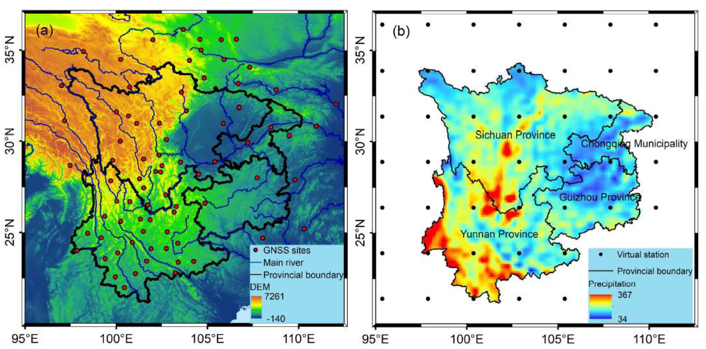
Figure 2.
Vertical displacement time series of four stations before and after preprocessing.
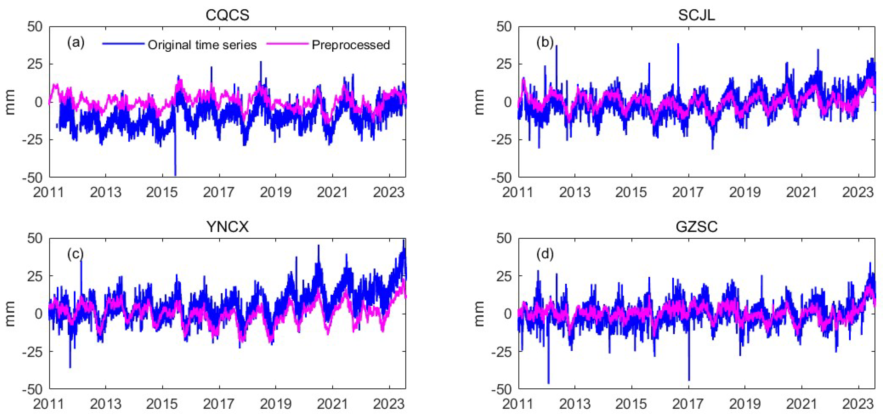
Figure 3.
Multi-source precipitation, evapotranspiration and runoff data.
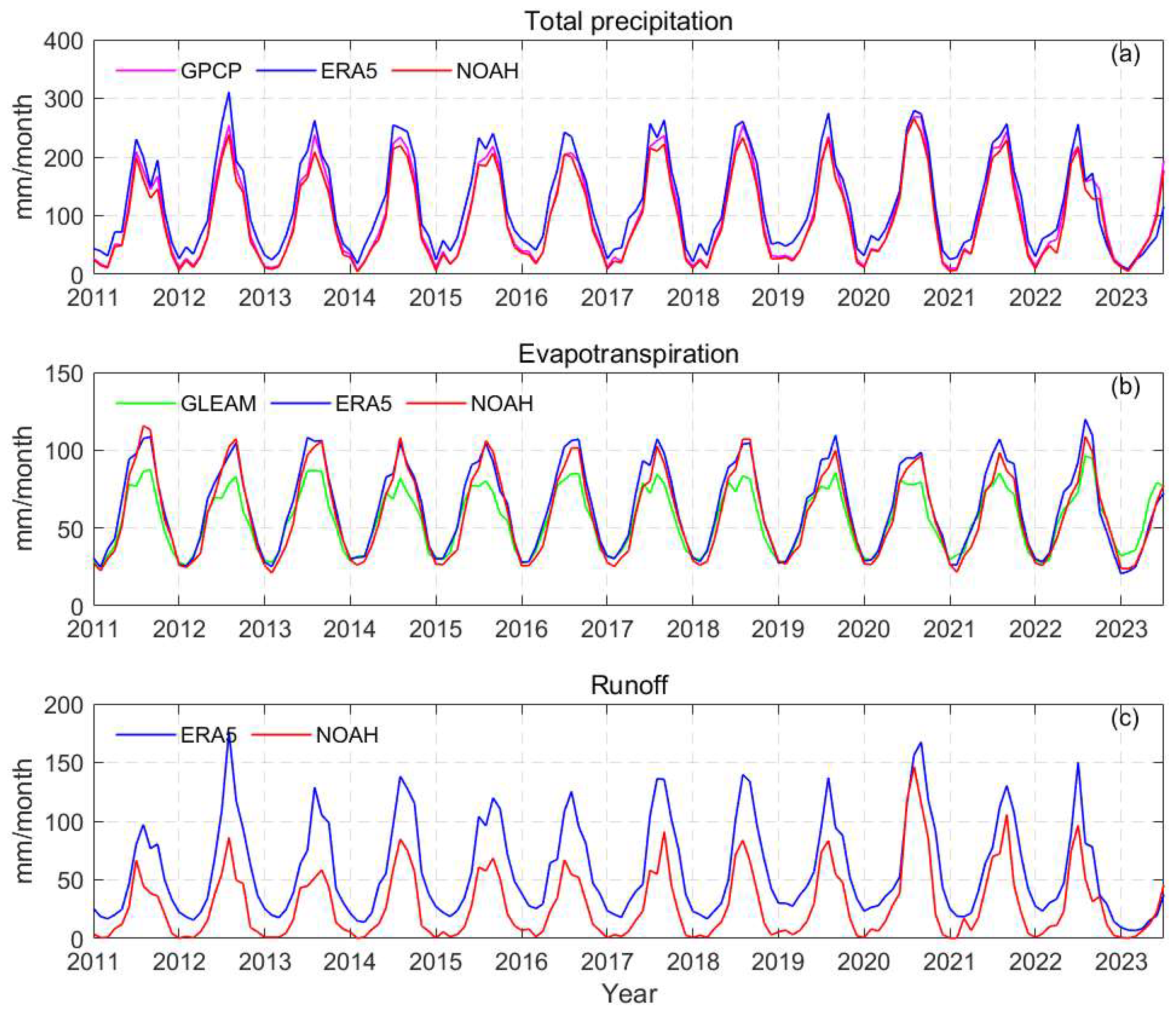
Figure 4.
ABIC value distribution.
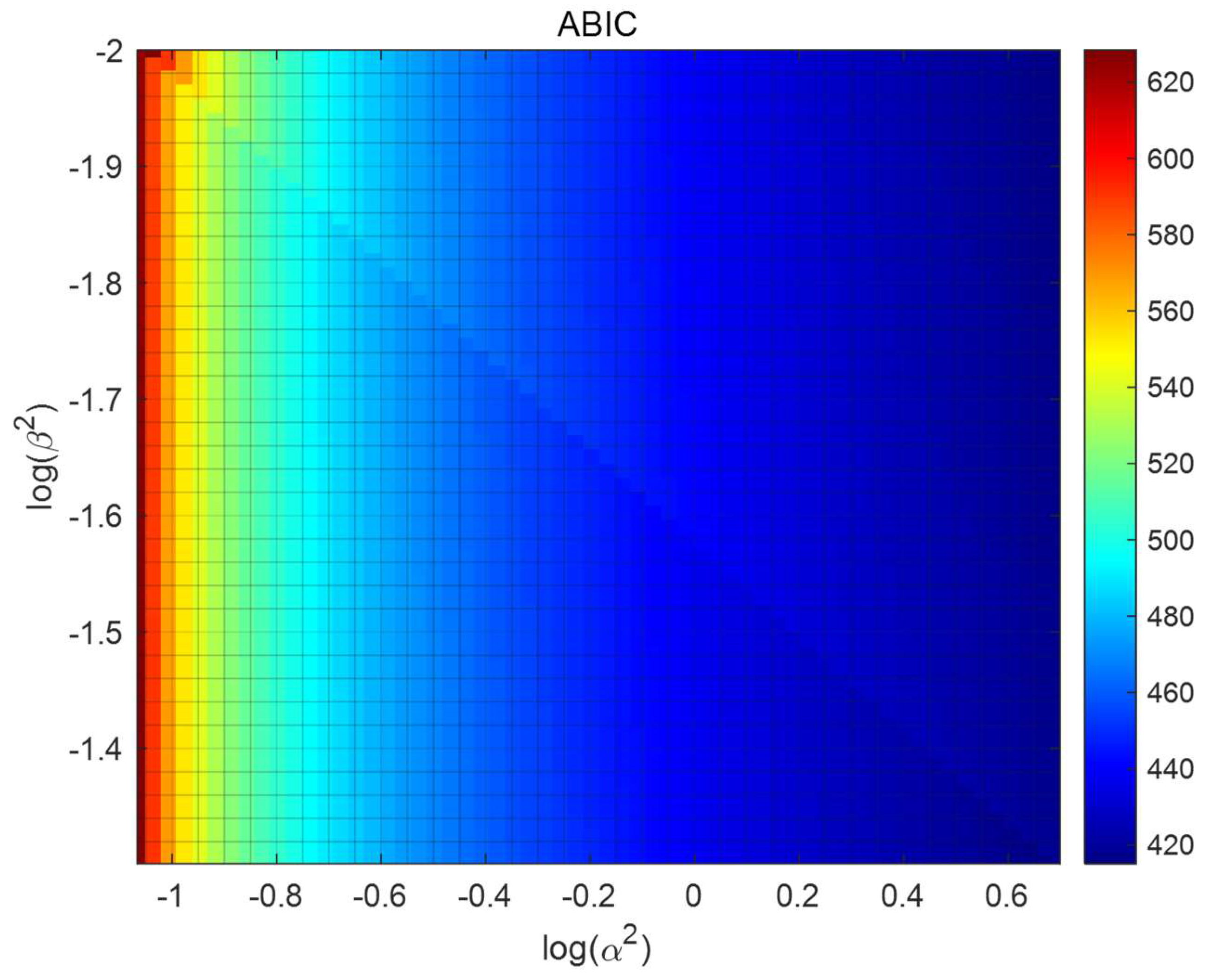
Figure 5.
Technical flowchart.
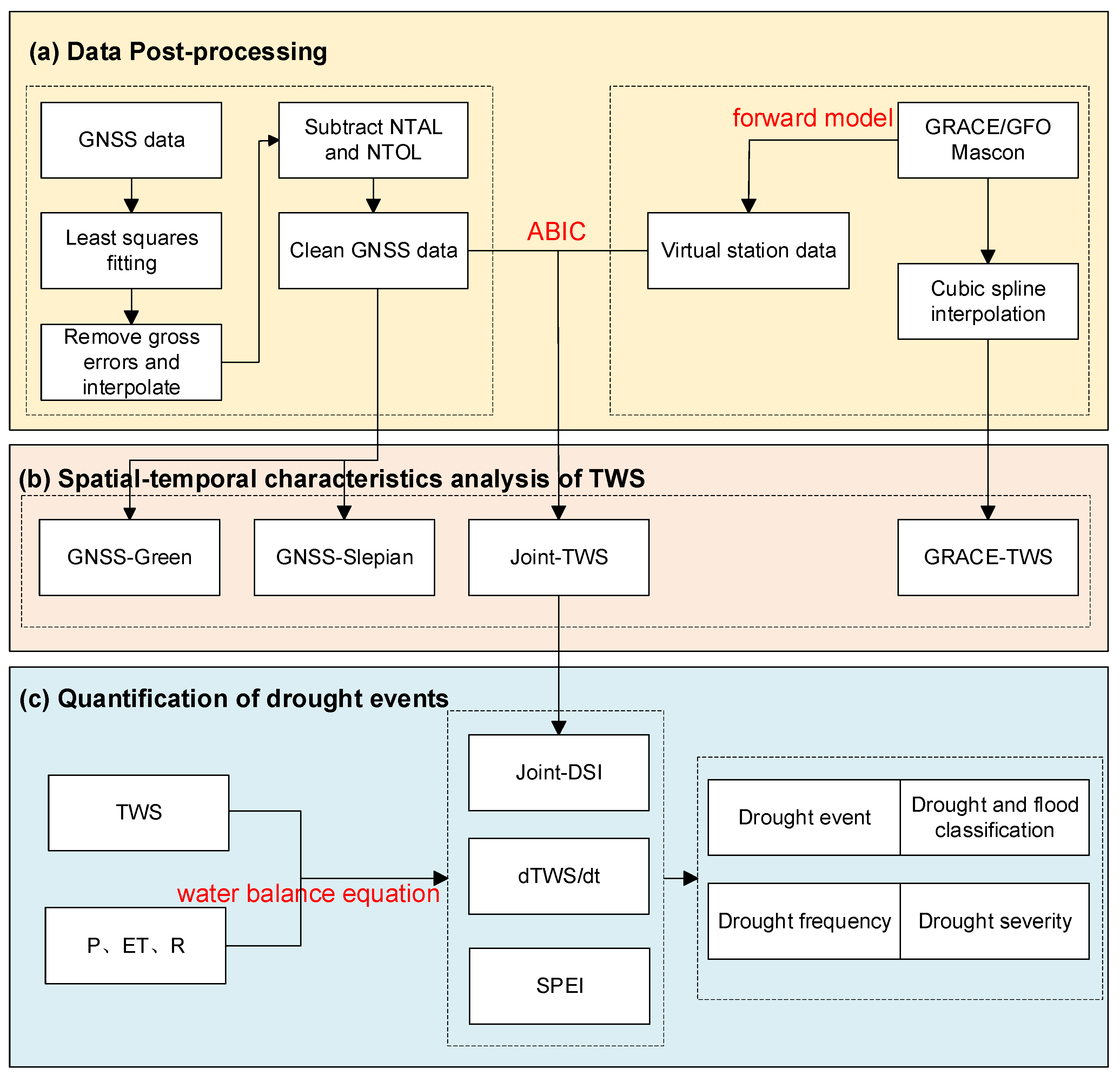
Figure 6.
Spatial distribution of TWS annual amplitude obtained by different inversion methods (GNSS-Green, GNSS-Slepian, GRACE, and Joint) in Southwest China from December 2010 to June 2023. The red dots indicate the GNSS stations and the green dots indicate the GRACE/GFO virtual stations.
Figure 6.
Spatial distribution of TWS annual amplitude obtained by different inversion methods (GNSS-Green, GNSS-Slepian, GRACE, and Joint) in Southwest China from December 2010 to June 2023. The red dots indicate the GNSS stations and the green dots indicate the GRACE/GFO virtual stations.
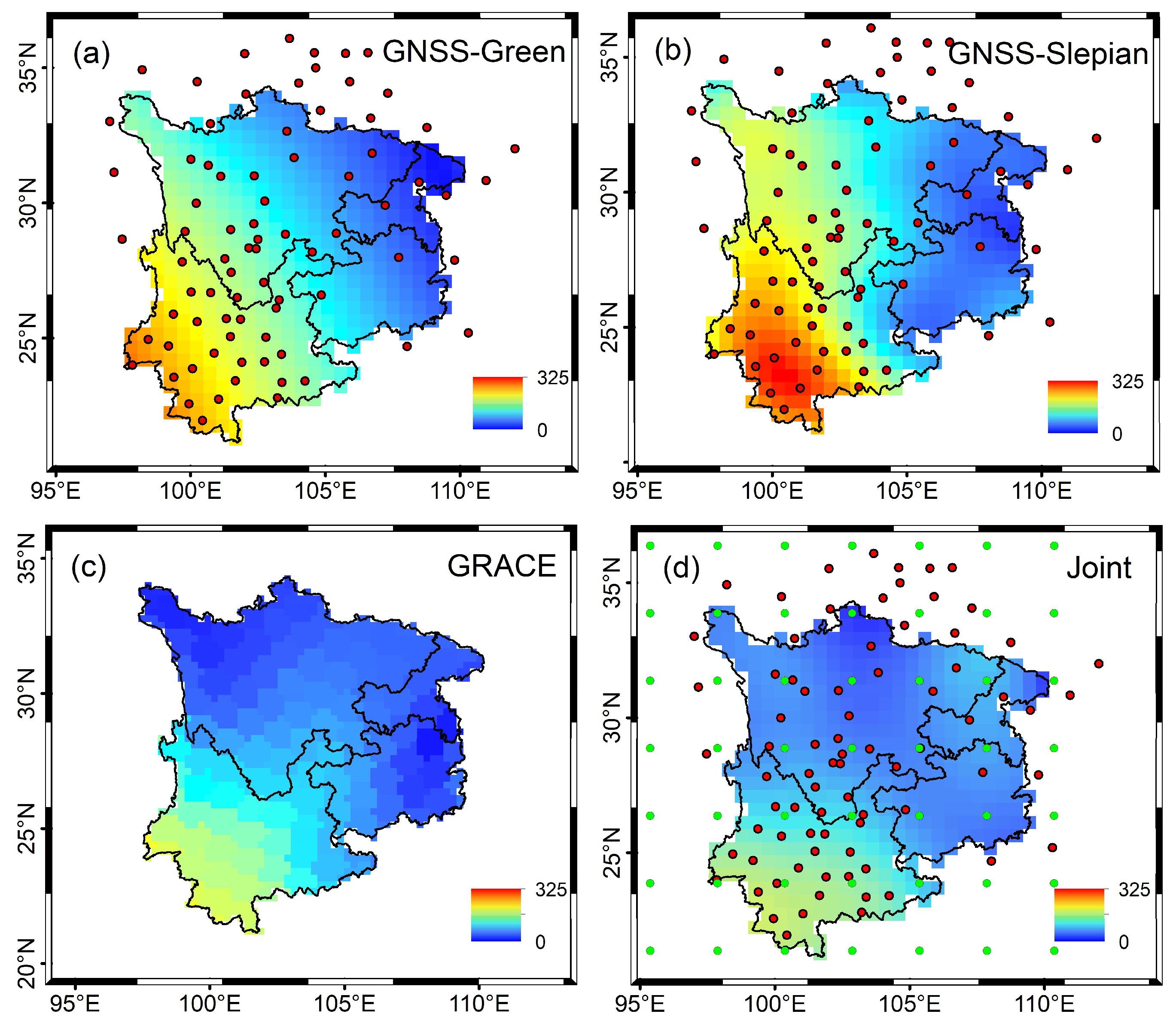
Figure 7.
Spatial distribution of TWS annual phase obtained by different inversion methods (GNSS-Green, GNSS-Slepian, GRACE, and Joint) in Southwest China from December 2010 to June 2023.
Figure 7.
Spatial distribution of TWS annual phase obtained by different inversion methods (GNSS-Green, GNSS-Slepian, GRACE, and Joint) in Southwest China from December 2010 to June 2023.
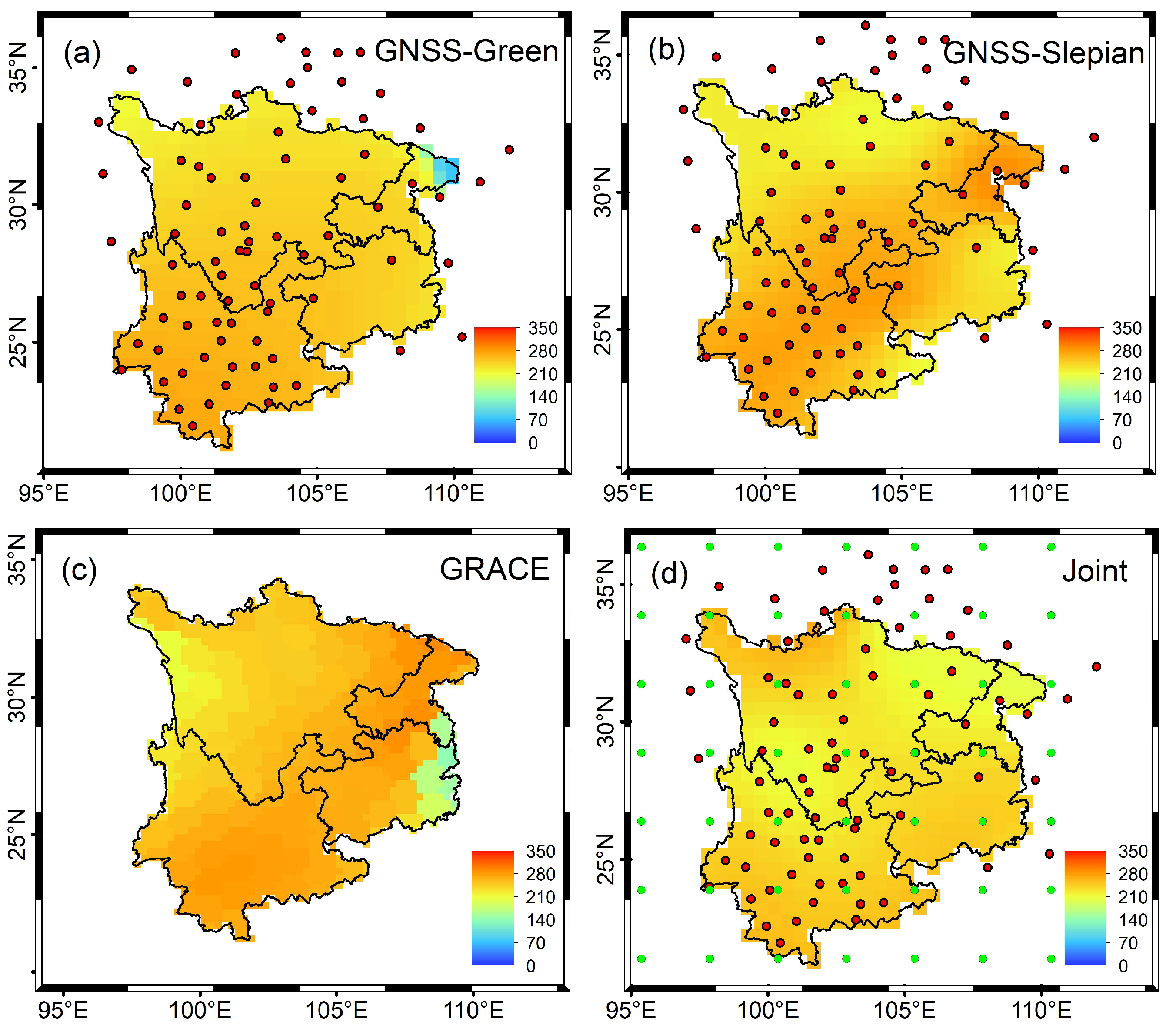
Figure 8.
(a) Time series of TWS changes and precipitation obtained by GNSS-Green, GNSS-Slepian, GRACE, and Joint methods; (b) Time series of dTWS/dt derived from GNSS-Green, GNSS-Slepian, GRACE, Joint methods, and ERA5 datasets and NOAH data.
Figure 8.
(a) Time series of TWS changes and precipitation obtained by GNSS-Green, GNSS-Slepian, GRACE, and Joint methods; (b) Time series of dTWS/dt derived from GNSS-Green, GNSS-Slepian, GRACE, Joint methods, and ERA5 datasets and NOAH data.
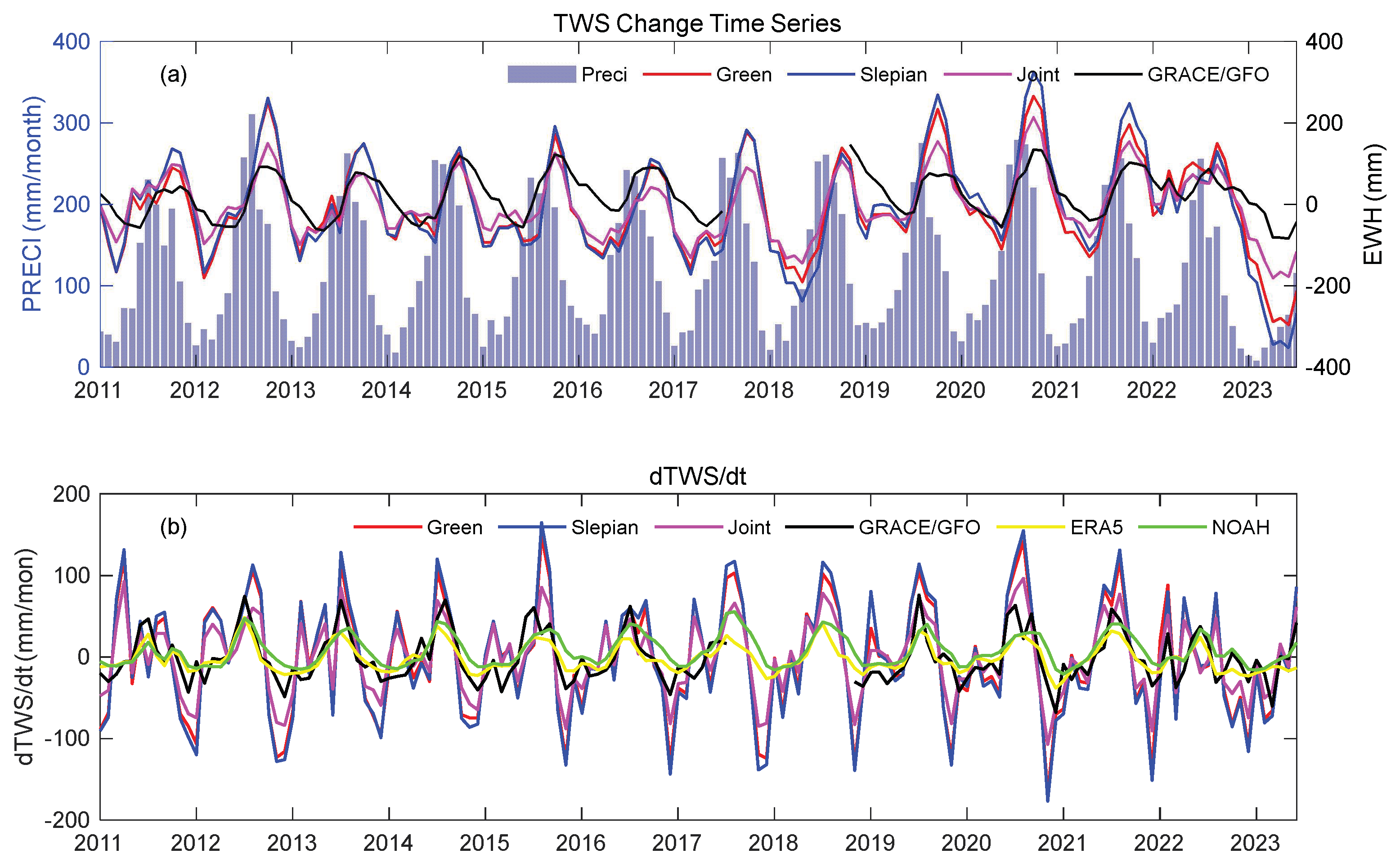
Figure 9.
Temporal variations of Joint-DSI, SPEI, and precipitation deficit on a monthly scale across four provinces and municipalities in Southwest China.
Figure 9.
Temporal variations of Joint-DSI, SPEI, and precipitation deficit on a monthly scale across four provinces and municipalities in Southwest China.
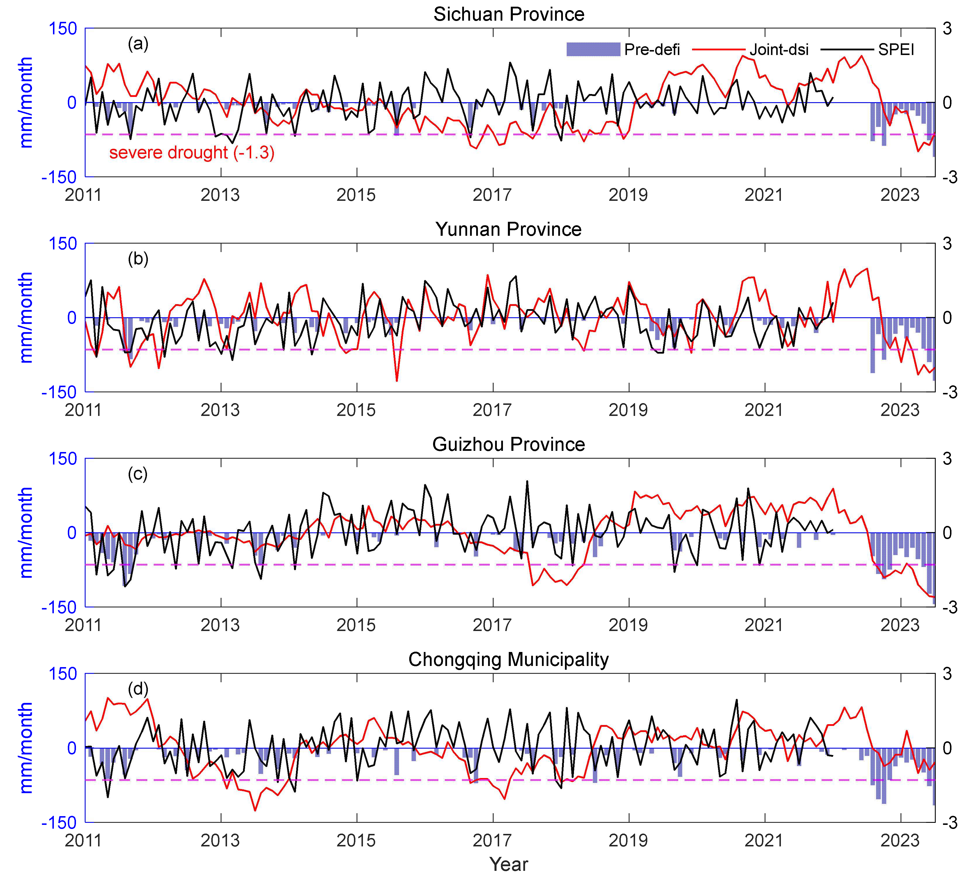
Figure 10.
Joint inversion checkerboard test results.
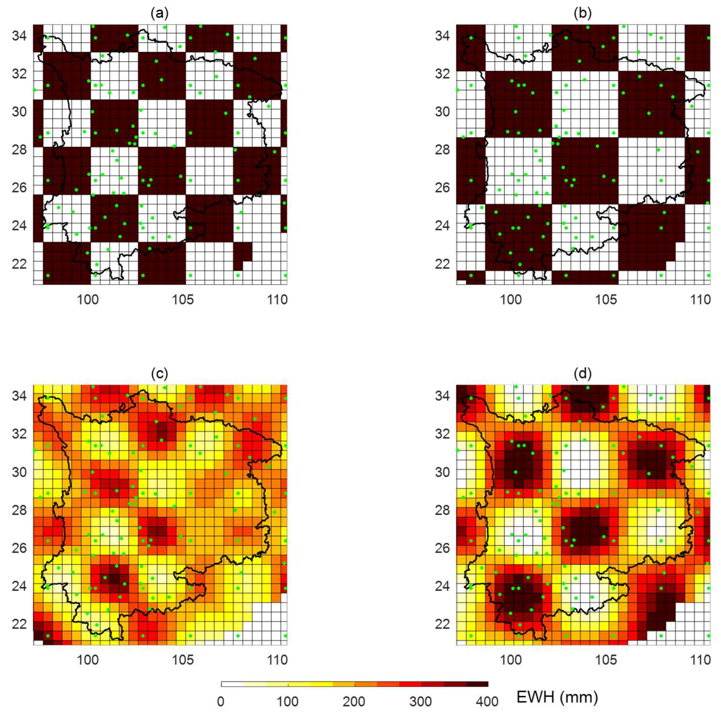
Figure 11.
Drought and flood classification based on Joint-DSI time series across four provinces and municipalities in Southwest China.
Figure 11.
Drought and flood classification based on Joint-DSI time series across four provinces and municipalities in Southwest China.
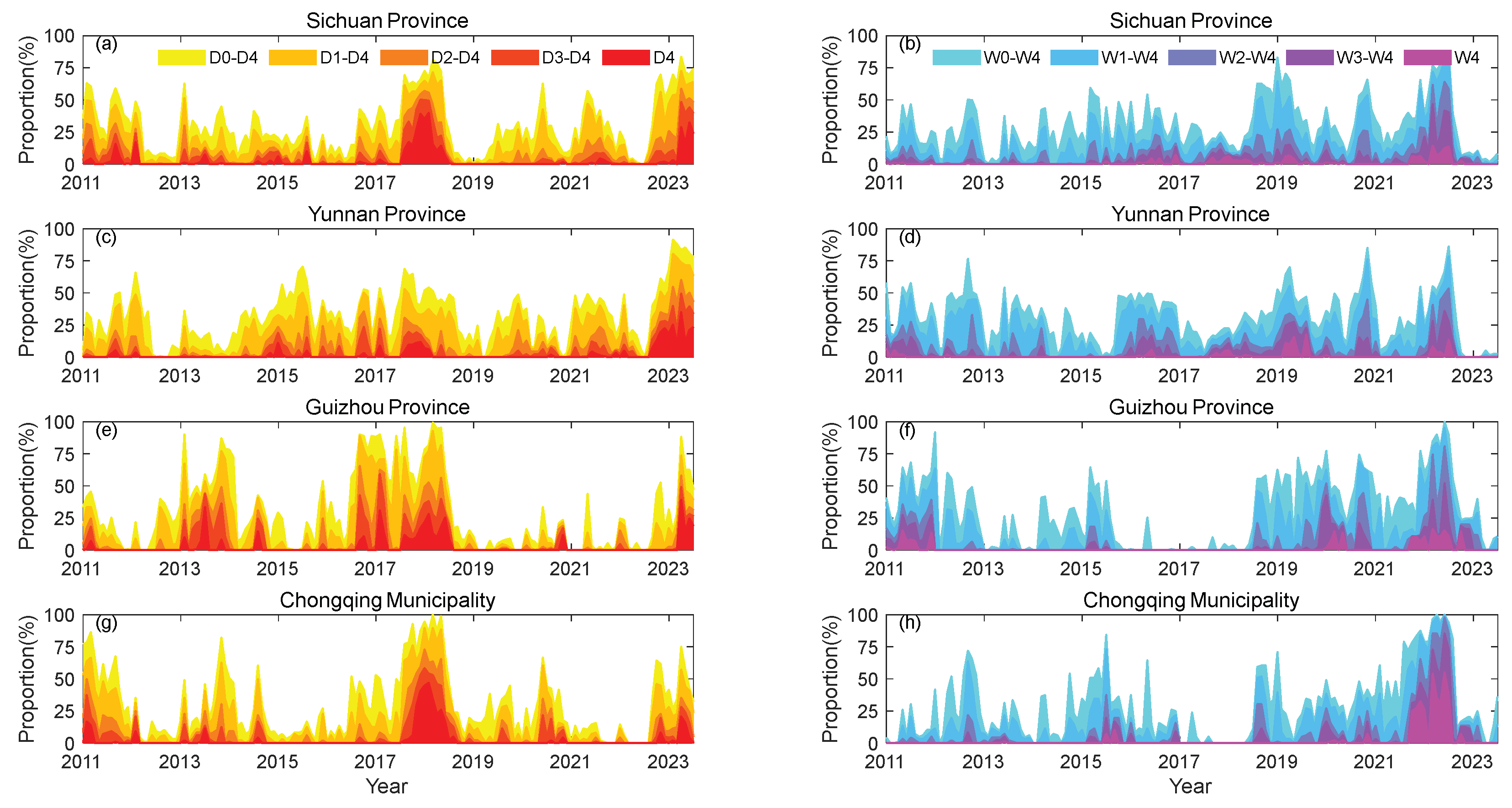
Figure 12.
Joint-DSI drought frequency distribution on a monthly scale. (a) represents the drought frequency distribution for 151 months from December 2010 to June 2023; (b) represents the drought frequency distribution for 12 months from July 2022 to June 2023.
Figure 12.
Joint-DSI drought frequency distribution on a monthly scale. (a) represents the drought frequency distribution for 151 months from December 2010 to June 2023; (b) represents the drought frequency distribution for 12 months from July 2022 to June 2023.
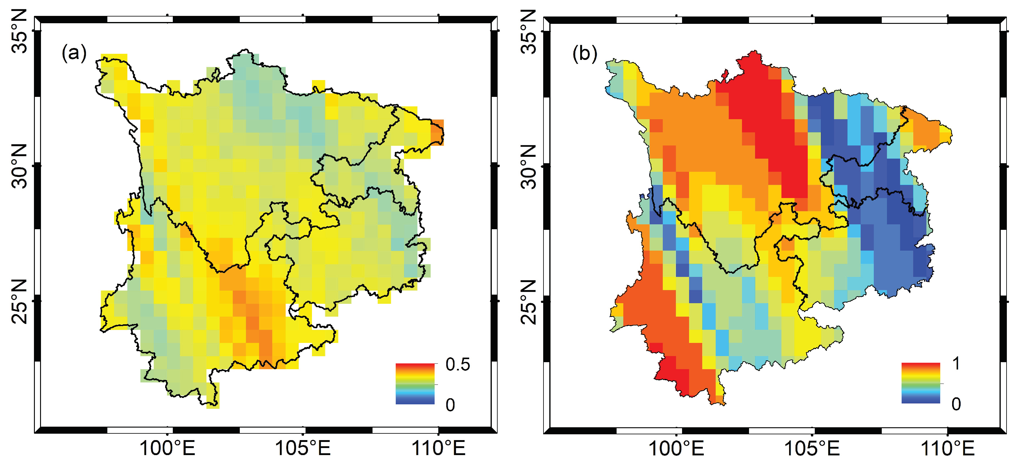

Table 1.
Correlation coefficients between dTWS/dt obtained from different datasets.
| GNSS-Green | GNSS-Slepian | Joint-TWS | GRACE-TWS | ERA5 | NOAH | |
|---|---|---|---|---|---|---|
| GNSS-Green | - | - | - | - | - | - |
| GNSS-Slepian | 0.99 | - | - | - | - | - |
| Joint-TWS | 0.98 | 0.98 | - | - | - | |
| GRACE-TWS | 0.66 | 0.66 | 0.69 | - | - | - |
| ERA5 | 0.61 | 0.62 | 0.62 | 0.79 | - | - |
| NOAH | 0.49 | 0.51 | 0.49 | 0.76 | 0.85 | - |
Table 2.
Drought events and severity inferred by Joint-TWS in Southwest China from December 2010 to June 2023.
Table 2.
Drought events and severity inferred by Joint-TWS in Southwest China from December 2010 to June 2023.
| Occurrence time | Duration (month) | Peak deficit (km3) | Average deficit (km3) | Total severity (km3) |
|---|---|---|---|---|
| 2013.08-2013.12 | 5 | -50.817(201310) | -32.899 | -164.499 |
| 2014.06-2015.01 | 8 | -22.758(201410) | -13.223 | -105.782 |
| 2015.05-2015.08 | 4 | -56.075(201507) | -23.912 | -95.649 |
| 2016.01-2018.12 | 36 | -111.192(201804) | -39.177 | -1410.370 |
| 2022.09-2023.06 | 10 | -150.694(202305) | -86.133 | -861.332 |
Disclaimer/Publisher’s Note: The statements, opinions and data contained in all publications are solely those of the individual author(s) and contributor(s) and not of MDPI and/or the editor(s). MDPI and/or the editor(s) disclaim responsibility for any injury to people or property resulting from any ideas, methods, instructions or products referred to in the content. |
© 2024 by the authors. Licensee MDPI, Basel, Switzerland. This article is an open access article distributed under the terms and conditions of the Creative Commons Attribution (CC BY) license (http://creativecommons.org/licenses/by/4.0/).
Copyright: This open access article is published under a Creative Commons CC BY 4.0 license, which permit the free download, distribution, and reuse, provided that the author and preprint are cited in any reuse.


