

Submitted:
06 December 2024
Posted:
09 December 2024
Read the latest preprint version here
Abstract
It may be helpful to integrate multiple aircraft communication and navigation functions into a single software defined radio (SDR) platform. To transmit these multiple signals, the SDR would first sum the baseband version of the signals. This outgoing composite signal would be passed through a digital-to-analog converter (DAC), before being up-converted and passed through a radio frequency (RF) amplifier. To prevent non-linear distortion in the RF amplifier, it is important to know the peak voltage of the composite. While this is reasonably straightforward when a single modulation is used, it is more challenging when working with composite signals. This paper describes a machine learning solution to this problem. We demonstrate that a generalized gamma distribution (GGD) is a good fit for the distribution of the instantaneous voltage of the composite waveform. A deep neural network was trained to estimate the GGD parameters, based on the parameters of the modulators. This allows the SDR to accurately estimate the peak of the composite voltage, and set the gain of the DAC and RF amplifier, without having to generate or directly observe the composite signal.
Keywords:
gain estimation
; digital to analog converter
; software defined radio
; aircraft communication
; signal processing
; deep learning
1. Introduction
Aerospace vehicles often require multiple connectivity applications for navigation, telemetry, communications, and a host of other applications [1]. As shown in Figure 1, these links may be through air-to-ground, satellite, and with other high altitude platforms and networks [1]. Legacy systems that use dedicated hardware devices for each link can be difficult to integrate and maintain. Interconnecting these systems can require wiring harnesses that substantially increase the weight and cost of the vehicle [2]. These costs, coupled with the complexities of modifying, integrating, troubleshooting, and maintaining new applications within hardware-dependent systems—especially those with extensive cabling—pose significant operational challenges [3].
Software-defined radios (SDR) allow designers to support multiple communication protocols on a single hardware platform. An SDR can generate multiple baseband waveforms for the various links they support, and then in a single operation up-convert and transmit them using a single hardware transmitter [4]. Amrhar et al. demonstrated that an SDR-based integrated modular avionics architecture could significantly reduce the size, weight, power usage, and cost in an aircraft [5]. The flexibility of reprogramming an SDR without hardware changes can give designers greater flexibility and assist in the troubleshooting and maintenance processes.
Multiple radio waveforms can be generated in a single SDR as illustrated in Figure 2. In this system, the SDR generates waveforms for each application then sums them into a single digital waveform. A digital-to-analog converter (DAC) produces an outgoing composite analog signal, which is up-converted and transmitted. To minimize quantization error, while still avoiding the nonlinear clipping of large signals, it is important to carefully select the input gain of the DAC. The composite signal’s peak amplitude is a key determinant of the optimal gain setting (), where V represents the DAC’s range and uV denotes the peak voltage of the composite signal, as further illustrated in Figure 3.
Estimating the DAC’s gain for an individual signal is relatively straightforward, as the peak amplitude is generally well-understood, even considering distortion from a pulse-shaping filter. The estimate can become challenging for composite signals due to the varied characteristics of each component signal, such as modulation technique, power level, and bit rate. One method for gain estimation involves a closed-loop system, adjusting the gain after the signal has been observed for some time. The signal may suffer from high quantization noise, or clipping, during the time required for the loop to reach the optimal level. The SDR could perform this operation in advance of having to transmit data, but that could substantially increase the SDR’s computational load.
To overcome this challenge, we propose a deep learning (DL) based technique to estimate statistical distribution of composite signal’s amplitudes. Our method relies exclusively on the parameters used to generate the component signals such as: modulation type, power levels, data rates, normalized carrier frequencies, and the number of applications; thereby, eliminating the need to generate or observe the composite signal to estimate DAC’s gain. This approach dynamically adapts the gain of the DAC to rapid changes in SDR configuration, ensuring use of DAC’s full range across varying scenarios.
Deep learning (DL) has grown in popularity in recent years due to the dramatic increase in the availability of computing power [6,7]. This success has led to an increased interest in the application of DL in communications and signal processing [8,9]. For instance, convolutional neural networks (CNNs) have been widely used for automatic modulation classification (AMC) by leveraging input features like constellation diagrams [10] and long-symbol rate signals [11]. Nambisan et al. [12] generated hybrid images using scalograms and IQ plots to reduce training time through transfer learning. Similarly, CNNs have been applied for channel state information (CSI) estimation by treating the time-frequency response of fast-fading channels as 2D images [13], while advanced architectures have integrated CNNs with long short-term memory (LSTM) networks for 5G wireless systems [14]. Attention-based mechanisms have also been employed for CSI estimation, using transformer encoder architectures to focus on critical features and improve performance [15]. Beyond CSI estimation, Ye et al. [16] demonstrated the use of deep neural networks (DNNs) for end-to-end channel estimation and symbol detection in orthogonal frequency-division multiplexing (OFDM) systems. Additionally, O’Shea et al. [17] trained an LSTM-based recurrent neural network for radio anomaly detection by predicting time-series data and comparing the expected error distribution with a well-characterized signal for non-anomalous behavior. Ma et al. [18] proposed an attention-based deep separation network for co-frequency modulated communication signals.
Another area where deep learning has shown promise is in regression-based applications, where deep neural network (DNN) regression models are used to estimate relationships between input and output variables. In particular, regression analysis is useful for predicting continuous-valued estimation targets based on a given D-dimensional vector x of independent input variables [19]. Sun et al. [20] demonstrated that a DNN can approximate signal processing algorithms by treating the input-output relationship as an unknown non-linear mapping, with training samples generated through optimization algorithms. This technique has also been applied in mobile terminal usage pattern estimation [21], as well as for CSI estimation [22]. The predictive power of regression analysis in estimating continuous variables makes it particularly useful for the task of estimating the statistical distribution parameters of composite signal amplitude levels in this study.
This article is an extension of [23], where the authors demonstrate a method to estimate DAC’s gain using statistical moments. This article demonstrates that a composite signal generated by summing signals with different modulation techniques, power levels, data rate, and normalized carrier frequency has voltage levels that adhere to the GGD [24]. We simulate a dataset of composite signals, calculating their respective GGD parameters. This dataset is utilized to train a DNN for regression, where the inputs are modulation technique, power level, data rate, the carrier frequency of each component signal, and the count of signals combined. The DNN’s output targets are the parameter values of the composite signal’s GGD.
The remainder of this paper is organized as follows: Section II discusses the generation of composite signals and their statistical distribution. Section III outlines the application of DNN regression for estimating the statistical distribution parameters of the summed signals. Section IV presents simulation results for the proposed multi-output DNN regression technique and compares these with other regression methods. Finally, Section V concludes the paper.
2. Composite Signal’s Distribution and the Dataset
This section describes how an outgoing composite signal is generated using multiple M-ary quadrature amplitude modulated (MQAM) signals. The residual sum of squares (RSS), and Kullback-Leibler (KL) divergence [25] are used to determine a theoretical distribution that closely fits the voltage distribution of the summed signal. This theoretical distribution is used to generate a dataset to train a DNN to estimate the distribution’s parameters.
2.1. Composite Signal
The composite signal is generated by adding multiple component signals with varying modulation orders, data rates, power levels, and normalized carrier frequencies. The number of component signals are chosen randomly between two and ten, inclusive. The component MQAM signal has the following form:
where is the MQAM signal, and are the in-phase and quadrature-phase amplitude levels, is the pulse shaping filter, is the baseband carrier frequency, and is the modulation order of MQAM signal. A composite signal can then be represented as:
where represents the composite signal, N is the number of MQAM signals added, and denotes the power factor.
The modulation order, M, of the MQAM component signals is uniformly sampled from the set of eight values described in Table 1. The data rate, power level, and normalized carrier frequency of the component signal are uniformly sampled from the ranges listed in Table 1, with power levels uniformly distributed on a dB scale and carrier offsets in increments of 1 kHz. Figure 4 shows the power spectrum of a representative composite signal generated by adding ten component signals.
2.2. Distribution Fitting
To determine a suitable statistical distribution for representing the voltage levels of composite signals, we first fit continuous statistical distributions listed in [26] to the data using RSS. The RSS score quantifies how well the fitted distribution replicates the individual sample data points by measuring the sum of the squared differences between the observed values () and the values predicted by the fitted distribution (). The RSS score, , is defined as:
where K is the number of data samples, is the data sample, and is an estimate of from the fitted distribution. The parameters for each candidate distribution are optimized by minimizing , which provides the closest fit of the statistical distribution to the data.
Once the parameters of the fitted distributions were optimized using RSS, KL-divergence was calculated to evaluate how well the theoretical distribution, generated with the optimal estimated parameters, aligned with the composite signal’s voltage distribution. KL divergence measures the relative entropy between two probability distributions that indicates how much information is lost when the fitted distribution (Q) is used to approximate the true distribution of the signal (P). For discrete probability distributions P and Q, the KL divergence score from Q to P is defined as:
where P represents the composite signal’s samples, and Q represents theoretical distribution with optimal estimated parameters, and is the probability space. A lower value indicates a better approximation, with meaning that the fitted distribution Q is identical to the true distribution P.
To compare the quality of each fitted distribution, we computed the mean, , and standard deviation, , for both and scores across 1000 instances of composite signals. The standard deviation, , describes consistency of fit; a lower suggests that a distribution performed consistently well across different composite signal instances.
Table 2 highlights the four distributions with the lowest and scores, signifying their close approximation to the composite signals’ behavior. Figure 5 illustrates the probability density function (PDF) of these distributions when fitted to a composite signal comprised of ten component signals, illustrating the efficacy of each in modeling the signal’s statistical properties.
Given that the GGD consistently yielded the lowest combined and scores, we use it to represent the voltage distribution of composite signals. For a voltage level, v, the PDF and the cumulative distribution function (CDF) of v are described in (5) and (6) respectively as follows:
where s, a, and b are the parameters of the GGD, is the gamma function, and is the lower incomplete gamma function.
To link the DAC’s gain, G, with the PDF of the transmitted signal, we consider the DAC’s clipping level, , and aim to scale the signal’s amplitude to match based on a specific percentile of the GGD. The optimal DAC’s gain, G, can be defined as:
where represents the inverse CDF (quantile function) of the GGD for a given probability (e.g. the percentile), indicating the voltage level below which a specified percentage of the signal’s amplitude distribution lies. This calculation ensures the adjusted signal amplitude optimally utilizes the DAC’s dynamic range, minimizing the risk of clipping and quantization noise.
2.3. Dataset
To train machine learning algorithms for multi-output regression, a dataset D of R samples was simulated, where . First, R composite signals were generated by summing multiple component signals, where the parameters of the component signals were selected from Table 1. A minimum of two and a maximum of ten signals were added, where each signal had four features: modulation order, data rate, power level, and normalized carrier frequency. To ensure that categorical features have the same distance among each other in the feature space, we used the one-hot-encoding technique to encode the modulation technique and number of composite signals features. Each composite signal was described using features, of which 120 describe the component signal’s parameters (12 features for each component signal), and 9 one-hot-encoded features describe the number of component signals added.
A GGD distribution was fit on each of the combined signal to calculate GGD’s parameters, shape parameters a and b, and a scale parameter s. Each sample in D has an input vector of p descriptive variables , and an output vector of q target variables , where , , and . Overall, the simulated dataset can be described by R samples of of pairs of input and output vectors, i.e., .
3. DNN Regression
This task involves estimating the parameters of the GGD by learning a multi-output regression model from dataset D. We find a function, , that assigns q output targets, , for each given input vector, , of length p [27]. This is expressed as
where denotes the sample space of , and denotes the sample space of , .
A DNN was used as a multi-output regression technique for GGD’s parameter estimation. As shown in Figure 6, the DNN has an input dimension of for input feature vector . The input layer is followed by four dense/hidden layers with 224, 256, 448, and 64 units respectively. The final dense layer is followed by an output layer with neurons for estimating target vector , with the estimates denoted as .
All the dense layers, the input layer, and the output layer were preceded by a batch-normalization layer to standardize inputs to a layer for each mini-batch. Mini-batch size was set to 512, and an exponentially decaying learning rate was used with an initial learning rate of . The drop-out rate of the neurons in the network was set to to mitigate overfitting of the training data. The dense layers used the ReLU activation function, thresholding raw scores at 0 (i.e. ), while the output layer employed a linear activation function, leaving raw scores unchanged (i.e. ). The number of layers, their corresponding number of neurons, batch size, learning rate, and drop-out rate were determined using Bayesian hyperparameter optimization technique [28].
4. Experiments, Results, and Analysis
This section outlines the methodology used to train the DNN and the outcomes of deploying it for estimating GGD’s parameters in composite signals. We suggest using a small deep neural network (S-DNN) that achieves performance comparable to the DNN with a sufficiently large number of SDR applications. A typical example is provided to demonstrate the use of the DNN estimates.
4.1. K-Fold Cross Validation
We implemented a 10-fold cross validation technique to use all training samples while performing robust validation [29]. Ten percent of the dataset was set aside for a hold-out test set. The remaining of the dataset was divided into ten equal folds. We trained the DNN ten times, using nine different folds, leaving out one fold for validation each time.
Mean Absolute Error (MAE) was used to quantify errors between the target values and the predictions at the output layer. The error values were then used to perform gradient descent to update the network’s weights. Early stopping, set with a patience of 100 epochs and a precision threshold of , was used to halt training when the validation set’s MAE ceased to significantly improve. Figure 7 illustrates the training and validation set’s average MAE trend, averaged across the ten folds, along with the minimum average validation MAE.
4.2. Performance of the DNN
We employed several metrics to evaluate the accuracy of the DNN in estimating the parameters of the GGD: value, explained variance, mean-squared error (MSE), and MAE. Table 3 summarizes the metric scores for each distribution parameter, along with the overall scores on all three parameters. The DNN demonstrates the highest accuracy in estimating the scale parameter s, achieving an of 0.9985 and an MAE of 0.0109 on the test set. The similarity between the and explained variances scores indicates that the mean of the error is close to zero. This suggests that the estimation of the distribution parameters by the DNN are largely unbiased, which implies the DNN is less prone to overestimation or underestimation. Figure 8 reveals the DNN’s challenges in accurately predicting parameter a values beyond 0.8. The scatter for parameters a and b appears more dispersed compared to that for parameter s, with parameter b showing the largest contribution to overall MAE and MSE. This discrepancy is likely due to the higher target values for parameter b, resulting in greater error magnitudes. Additionally, the smaller magnitude of parameter a compared to parameters b and s reduces its relative contribution to the loss function during training, leading to less precise estimates and contributing to the increased scatter observed in Figure 8.
Figure 9 illustrates the impact of training data volume on the DNN’s test set accuracy, as measured by the MAE. We observe a marked decrease in the overall MAE as the proportion of data used for training increases, showcasing rapid improvements in model accuracy. The rate of MAE reduction diminishes when training involves more than 50% of the data. Beyond this point, additional data yields only marginal improvements in accuracy, especially for parameters a and s. Marginal gains can be seen for parameter b until all the training data is exhausted, suggesting that parameter b’s estimates can potentially benefit from additional training data. The trends suggest that increasing the dataset size can enhance model performance, but there exists a threshold beyond which the benefits become incremental.
4.3. Model Interpretability
Model interpretability is essential, especially in critical applications like aviation. To interpret the contributions of input features to the model’s predictions we employed SHAP (SHapley Additive exPlanations) [30], which assigns an importance value to each feature, thereby explaining the model’s decisions. We grouped the input features into five primary categories: modulation order, data rate, power level, normalized carrier frequency, and number of component signals.
Table 4 presents the normalized SHAP values (percentage importance) for each feature group across the estimated distribution parameters a, b, and s, as well as the overall importance. These values indicate the relative contribution of each feature group to the model’s predictions.
The results demonstrate that modulation order and power level are the most influential features, each contributing approximately to the overall model predictions. The number of component signals in a particular composite signal also has a notable impact, contributing around . In contrast, data rate and normalized carrier frequency have minimal impact on the overall estimation but are more influential when estimating the shape parameter a.
4.4. Performance as Number of SDR Applications Increase
Figure 10 and Figure 11 demonstrate how the MAE and score change as components are added to the composite signal. The performance of the DNN is worse when trying to estimate distribution parameters for less than six component signals, especially for the shape parameters. Figure 10 shows that estimates of the shape parameter, s, become less accurate as more component signals are added to the composite signal, suggesting a trade off between shape and scale parameters as the number of SDR applications increase.
4.5. SMALL DNN
Implementing a DNN with 992 hidden-layer neurons across four hidden layers poses significant computational training costs. To assess efficiency, its performance was compared with that of the S-DNN, with 100 neurons distributed over three hidden layers (50, 30, and 20 neurons, respectively). Despite using only a tenth of the neurons, the S-DNN achieved an of , which is 4.13% lower than that of the DNN.
Figure 12 compares performance of the S-DNN with the DNN as the number of component signals increase. The SNN has significantly lower accuracy estimating shape parameter a, when there are fewer than six component signals. When seven or more component signals are used, the SNN has comparable performance to the DNN. This provides an alternative to use a model with considerably fewer parameters when an SDR is supporting sufficiently large number of applications.
4.6. Computational Resources and Model Complexity
The DNN and S-DNN models were trained on a personal computer equipped with an Intel Core i7-12700 CPU at 2.10 GHz, 32 GB of RAM, and an NVIDIA GeForce RTX 3060 TI GPU. Table 5 lists the training time for a training set of samples and the total number of floating point operations (FLOPs) required per inference for the two models.
The modest number of FLOPs, especially for the S-DNN, combined with manageable training times, indicate that the proposed models are practical for implementation in real-world SDR systems. The reduced computational complexity of the S-DNN makes it particularly suitable for systems with limited computational resources or when rapid adaptation is required.
4.7. Comparison with Other Techniques
The performance of the proposed neural networks is compared with following multi-output regression techniques:
Table 6 presents scores achieved by these techniques, along with those obtained from S-DNN and DNN. We used Bayesian hyperparameter optimization was employed to search for optimal settings for these methods [28]. K-NR shows the lowest overall score, indicating its relative ineffectiveness in capturing the relationships between signal parameters and the distribution parameters. Except for K-NR, the techniques demonstrated strong predictive capabilities for the s parameter, with the lowest of achieved by LR.
The shape parameters a and b proved more challenging to estimate, requiring the use of more complex models like RFR and GBRT. While ensemble methods performed comparably to the proposed neural networks for parameter s, the neural networks displayed superior performance in estimating the shape parameters. This is critical, as the estimation of shape parameters significantly impacts the prediction of composite signal’s peak amplitudes.
4.8. TYPICAL EXAMPLE
To demonstrate a normative scenario, consider a composite signal generated by adding the signals described in Table 7. Figure 13 displays the CDF of the composite signal’s voltage levels, as estimated by the DNN. Within Figure 13, we explore three scenarios detailing the probabilities of surpassing specific voltage levels. For instance, of the voltage levels in the composite signal are above volts. Such insights can be valuable while determining DAC’s gain. For example, if DAC’s operational range is volts and G is the gain, then ensures that only of the signal samples will be clipped.
5. Conclusion
This study introduces a deep learning based approach to determine the optimal gain of a DAC in scenarios where an SDR generates multiple baseband signals for aircraft communications. We identified an analytical distribution that closely models the voltage distribution of the composite signal, using the RSS fitting method, and found that the GGD fits the composite signal particularly well. We trained a DNN on simulated composite signal data to estimate the parameters of the GGD. This trained DNN allows rapid prediction of the composite signal’s voltage distribution as it varies with changes in the SDR configuration. Utilizing the predicted voltage distribution, the DAC’s gain can be dynamically adjusted, maximizing its range utilization and minimizing potential signal distortion.
Author Contributions
Conceptualization, K.K.; data curation, V.K.; formal analysis, V.K.; investigation, V.K.; methodology, V.K.; project administration, K.K.; software, V.K.; supervision, K.K.; validation, V.K. and K.K.; visualization, V.K.; writing - original draft, V.K.; writing - reviewing & editing, V.K. and K.K. All authors have read and agreed to the published version of the manuscript.
Funding
This research received no external funding.
Data Availability Statement
The methodology used to simulate the data is described in the manuscript, further inquiries can be directed to the corresponding author.
Conflicts of Interest
The authors declare no conflicts of interest.
Abbreviations
The following abbreviations are used in this manuscript:
| SDR | Software Defined Radio |
| DAC | Digital to Analog Converter |
| RF | Radio Frequency |
| GGD | Generalized Gamma Distribution |
| DL | Deep Learning |
| DNN | Deep neural network |
| MQAM | M-ary Quadrature Amplitude Modulated |
| RSS | Residual Sum of Squares |
| KL | Kullback-Leibler |
| Probability Density Function | |
| CDF | Cumulative Density Function |
| S-DNN | Small-Deep Neural Network |
| MAE | Mean Absolute Error |
| MSE | Mean Squared Error |
| SHAP | SHapley Additive exPLanations |
| FLOP | Floating Point OPeration |
| LR | Linear Regression |
| K-NR | K-Neighbors Regression |
| DTR | Decision Tree Regression |
| RFR | Random Forest Regression |
| GBRT | Gradient Boosted Regression Trees |
| SVR | Support Vector Regression |
References
- Baltaci, A.; Dinc, E.; Ozger, M.; Alabbasi, A.; Cavdar, C.; Schupke, D. A survey of wireless networks for Future Aerial Communications (FACOM). IEEE Communications Surveys & Tutorials 2021, 23, 2833–2884. [CrossRef]
- Furse, C.; Haupt, R. Down to the wire [aircraft wiring]. IEEE Spectrum 2001, 38, 34–39. [CrossRef]
- Sámano-Robles, R.; Tovar, E.; Cintra, J.; Rocha, A. Wireless avionics intra-communications: Current trends and design issues. Eleventh ICDIM; , 2016; pp. 266–273.
- Price, N.; Kosbar, K. Decoupling hardware and software concerns in aircraft telemetry SDR systems. Proc. ITC; , 2018; pp. 474–483.
- Amrhar, A.; Kisomi, A.A.; Zhang, E.; Zambrano, J.; Thibeault, C.; Landry, R. Multi-Mode reconfigurable Software Defined Radio architecture for avionic radios. ICNS; , 2017; pp. 2D1–1–2D1–10.
- Pouyanfar, S.; Sadiq, S.; Yan, Y.; Tian, H.; Tao, T.; Reyes, M.P.; Shyu, M.; Chen, S.; Iyenger, S.S. A survey on deep learning: Algorithms, techniques, and applications. ACM Computing Surveys (CSUR) 2019, 51, 1–36. [CrossRef]
- Dong, S.; Wang, P.; Abbas, K. A survey on deep learning and its applications. Computer Science Review 2021, 40. [CrossRef]
- França, R.P.; Monteiro, A.; Arthur, R.; Iano, Y. An overview of deep learning in big data, image, and signal processing in the modern digital age. In Trends in Deep Learning Methodologies; Academic Press, 2020; pp. 63–87.
- Dai, L.; Jiao, R.; Adachi, F.; Poor, H.V.; Hanzo, L. Deep learning for wireless communications: An emerging interdisciplinary paradigm. IEEE Wireless Communications 2020, 27, 133–139. [CrossRef]
- Peng, S.; Jiang, H.; Wang, H.; Alwageed, H.; Zhou, Y.; Sebdani, M.M.; Yao, Y. Modulation classification based on signal constellation diagrams and deep learning. IEEE Transactions on Neural Networks and Learning Systems 2019, 30, 718–727. [CrossRef]
- Meng, F.; Chen, P.; Wu, L.; Wang, X. Automatic modulation classification: A deep learning enabled approach. IEEE Transactions on Vehicular Technology 2018, 67, 10760–10772. [CrossRef]
- Nambisan, A.; Gajjar, V.; Kosbar, K. Scalogram Aided Automatic Modulation Classification. Proc. ITC;
- Soltani, M.; Pourahmadi, V.; Mirzaei, A.; Sheikhzadeh, H. Deep learning-based channel estimation. IEEE Communications Letters 2019, 23, 652–655. [CrossRef]
- Luo, C.; Ji, J.; Wang, Q.; Chen, X.; Li, P. Channel State Information Prediction for 5G Wireless Communications: A Deep Learning Approach. IEEE Transactions on Network Science and Engineering 2020, 7, 227–236. [CrossRef]
- Luan, D.; Thompson, J. Attention Based Neural Networks for Wireless Channel Estimation. 2022 IEEE 95th Vehicular Technology Conference: (VTC2022-Spring), 2022, pp. 1–5. [CrossRef]
- Ye, H.; Li, G.Y.; Juang, B.H. Power of Deep Learning for Channel Estimation and Signal Detection in OFDM Systems. IEEE Wireless Communications Letters 2018, 7, 114–117. [CrossRef]
- O’Shea, T.J.; Clancy, T.C.; McGwier, R.W. Recurrent Neural Radio Anomaly Detection, 2016, [arXiv:cs.LG/1611.00301].
- Ma, H.; Zheng, X.; Yu, L.; Zhou, X.; Chen, Y. A novel end-to-end deep separation network based on attention mechanism for single channel blind separation in wireless communication. IET Signal Processing 2023, 17, e12173, [https://ietresearch.onlinelibrary.wiley.com/doi/pdf/10.1049/sil2.12173]. [CrossRef]
- Jiang, C.; Zhang, H.; Ren, Y.; Han, Z.; Chen, K.C.; Hanzo, L. Machine learning paradigms for next-generation wireless networks. IEEE Wireless Communications 2017, 24, 98–105. [CrossRef]
- Sun, H.; Chen, X.; Shi, Q.; Hong, M.; Fu, X.; Sidiropoulos, N.D. Learning to Optimize: Training Deep Neural Networks for Interference Management. IEEE Transactions on Signal Processing 2018, 66, 5438–5453. [CrossRef]
- Donohoo, B.K.; Ohlsen, C.; Pasricha, S.; Xiang, Y.; Anderson, C. Context-aware energy enhancements for smart mobile devices. IEEE Transactions on Mobile Computing 2014, 13, 1720–1732. [CrossRef]
- Gajjar, V.; Kosbar, K. CSI estimation using artificial neural network. Proc. ITC; , 2019; pp. 413–422.
- Gajjar, V.; Kosbar, K. Rapid gain estimation for multi-user software defined radio applications. Proc. ITC;
- Stacy, E.W. A generalization of the gamma distribution. The Annals of Mathematical Statistics 1962, 33, 1187–1192.
- Kullback, S.; Leibler, R. On information theory and sufficiency. The Annals of Mathematical Statistics 1951, 22, 79–86.
- Continuous Statistical Distributions — SCIPY V1.13.0 Manual.
- Borchani, H.; Varando, G.; Bielza, C.; Larranaga, P. A survey on multi-output regression. Wiley Interdisciplinary Reviews: Data Mining and Knowledge Discovery 2015, 5, 216–233. [CrossRef]
- Brochu, E.; Cora, V.M.; de Freitas, N. A Tutorial on Bayesian Optimization of Expensive Cost Functions, with Application to Active User Modeling and Hierarchical Reinforcement Learning. CoRR 2010, abs/1012.2599, [1012.2599].
- Ojala, M.; Garriga, G.C. Permutation tests for studying classifier performance. Journal of machine learning research 2010, 11.
- Lundberg, S.M.; Lee, S.I. A unified approach to interpreting model predictions. Proceedings of the 31st International Conference on Neural Information Processing Systems; Curran Associates Inc.: Red Hook, NY, USA, 2017; NIPS’17, p. 4768–4777.
- Montgomery, D.C.; Peck, E.A.; Geoffrey, G.G. Multiple linear regression. In Introduction to Linear Regression Analysis, 6 ed.; John Wiley and Sons, Inc.: Hoboken, NJ, USA, 2021; pp. 72–85.
- Kramer, O. K-Nearest Neighbors; Springer: Berlin, Germany, 2013; pp. 13–23.
- Dea’th, G. Multivariate regression trees: A new Technique for modelling species-environment relationships. Ecology 2002, 83, 1105–1117. [CrossRef]
- Segal, M.R. Machine learning benchmarks and random forest regression 2004.
- Prettenhofer, P.; Louppe, G. Gradient Boosted Regression Trees in Scikit-Learn. 23 February 2014.
- Brudnak, M. Vector-valued support vector regression. IEEE Int. Joint Conf. on Neural Network Proc.; , 2006; pp. 1562–1569.
Figure 1.
Typical communication links of an aircraft.
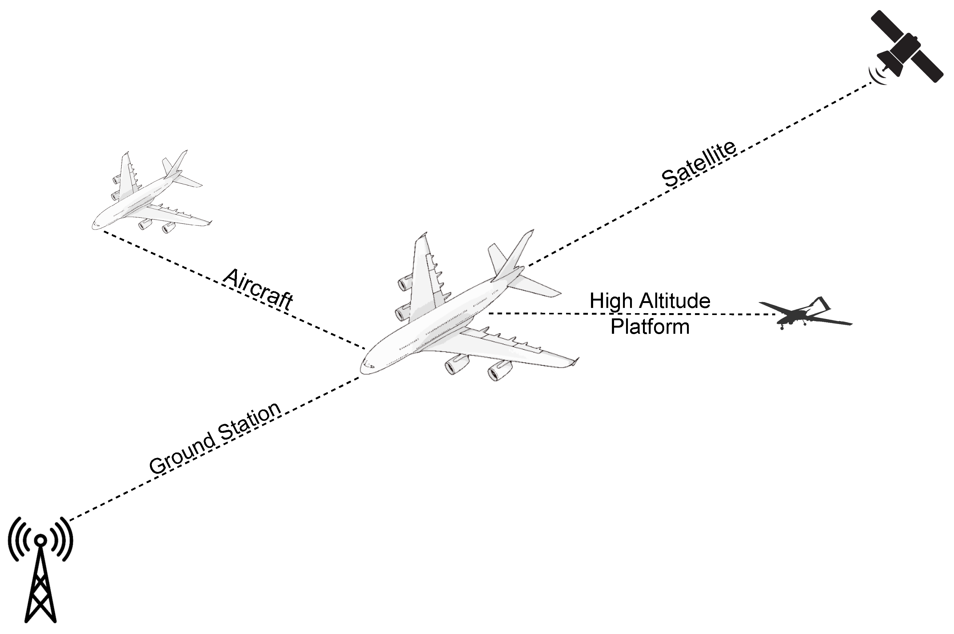
Figure 2.
SDR-Based Implementation of an Airplane’s Communication Links.
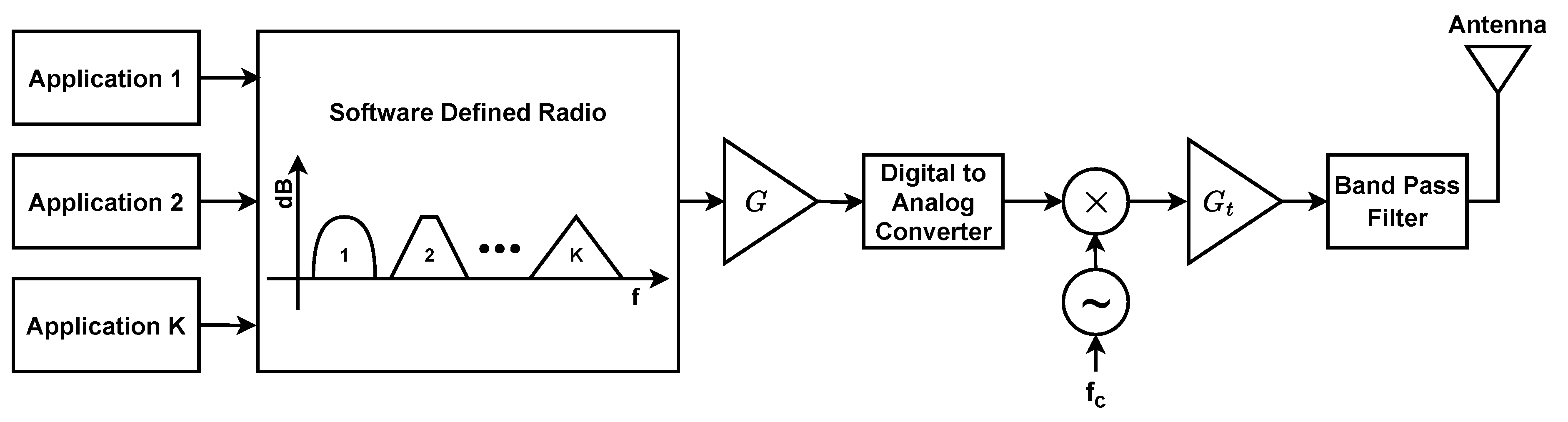
Figure 3.
Time domain representation of a composite signal.
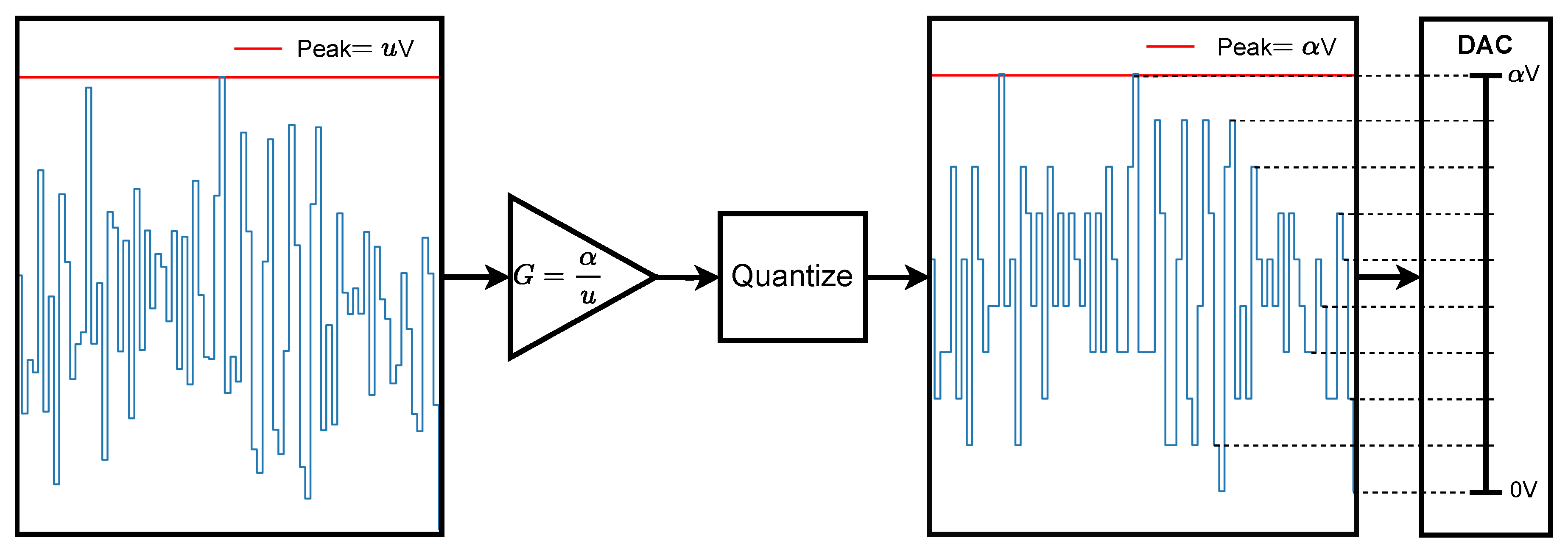
Figure 4.
Frequency domain representation of a composite signal.
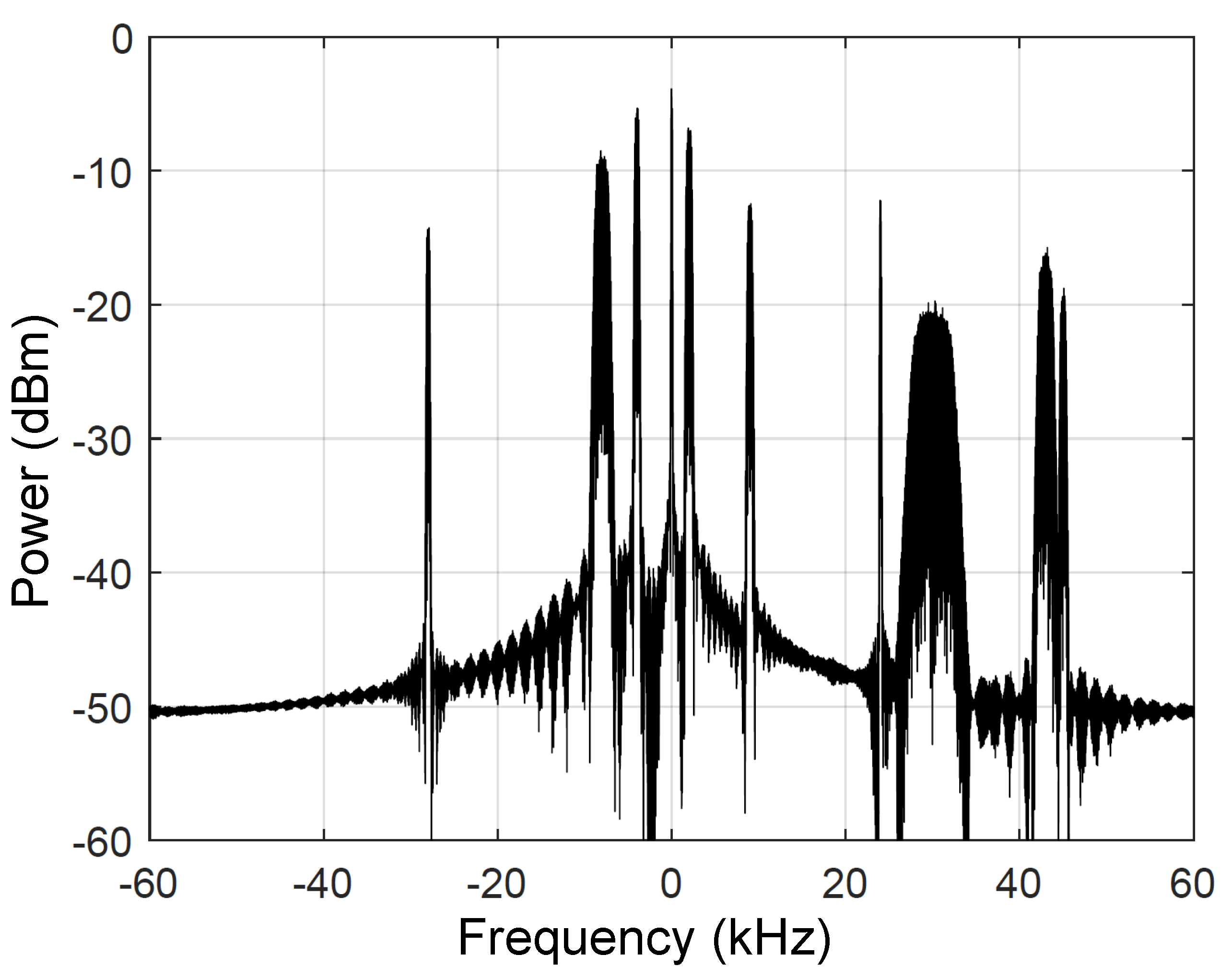
Figure 5.
Four common distributions that closely fit composite signals.
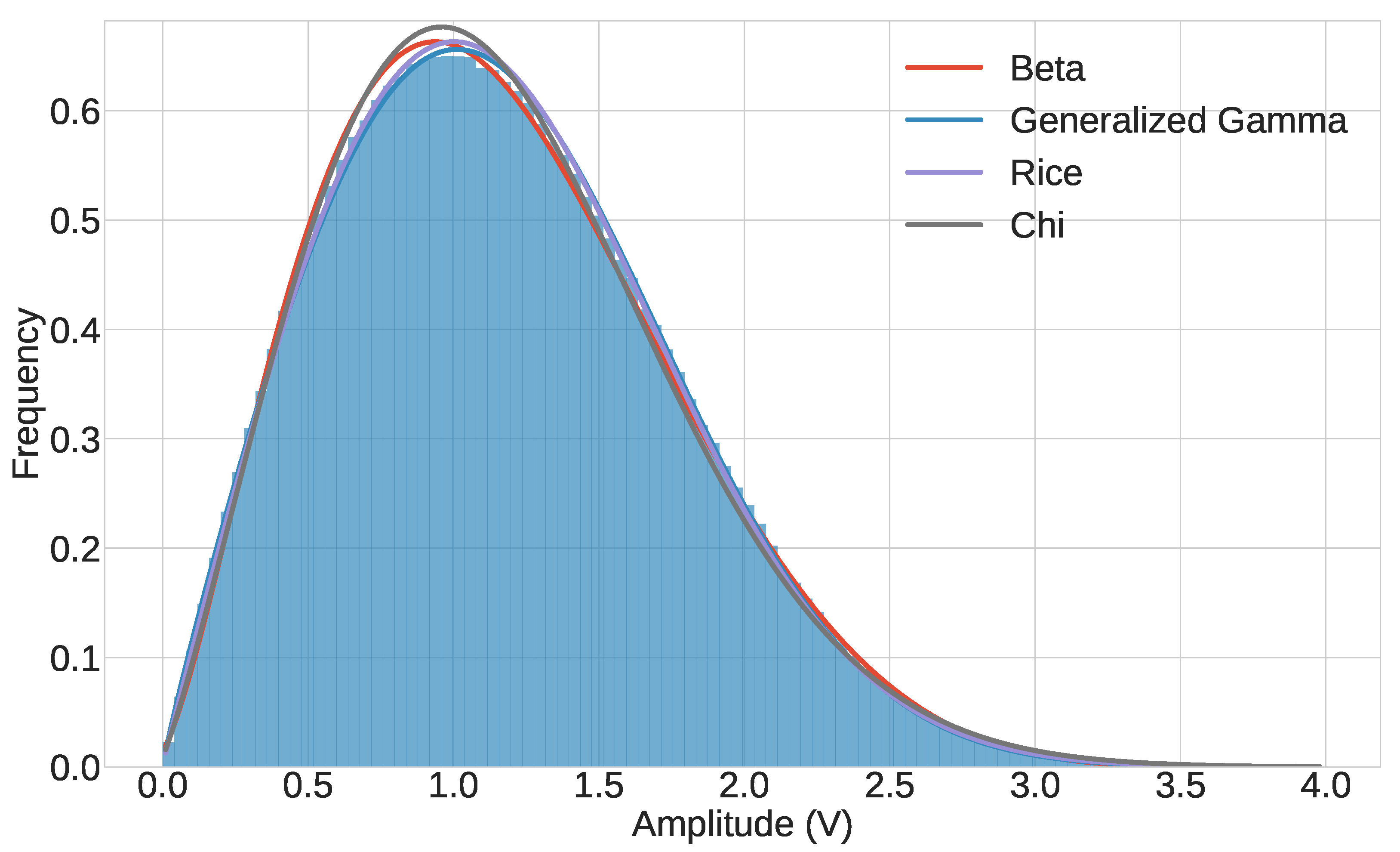
Figure 6.
DNN used to estimate GGD’s parameters.
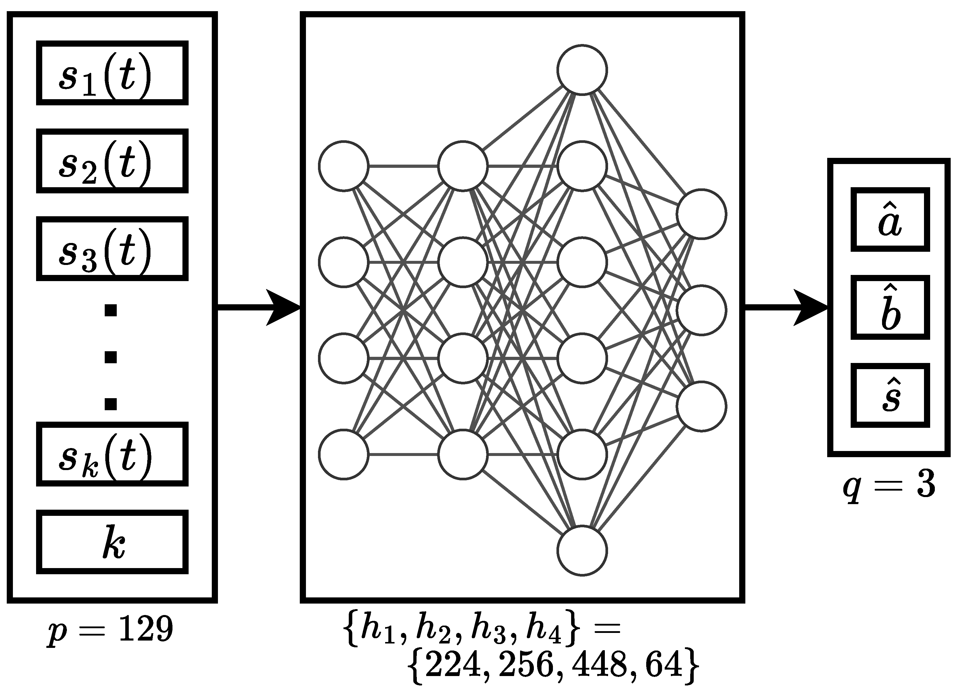
Figure 7.
Average MAE training and validation loss trends across 10-fold cross validation.
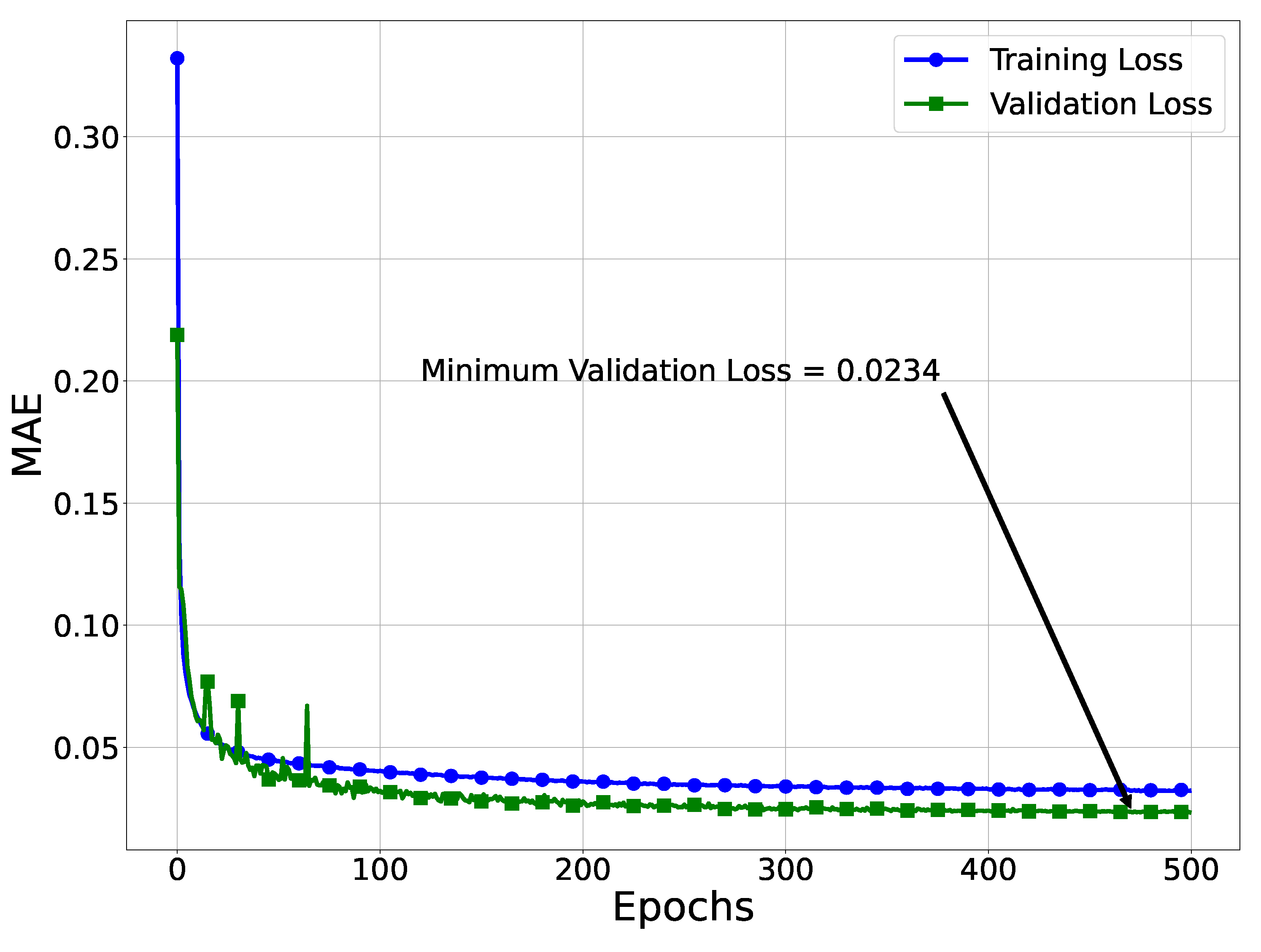
Figure 8.
plot for each of the individual parameters of the GGD, estimated using the DNN.
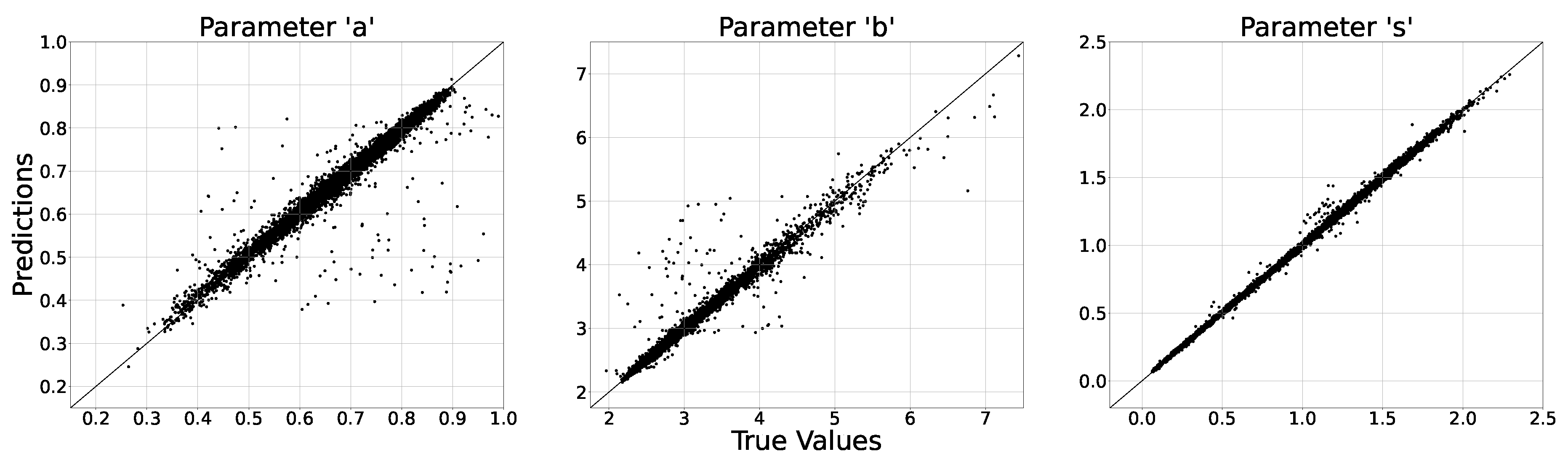
Figure 9.
Trend in MAE on the hold-out test set with increasing amount of training data.
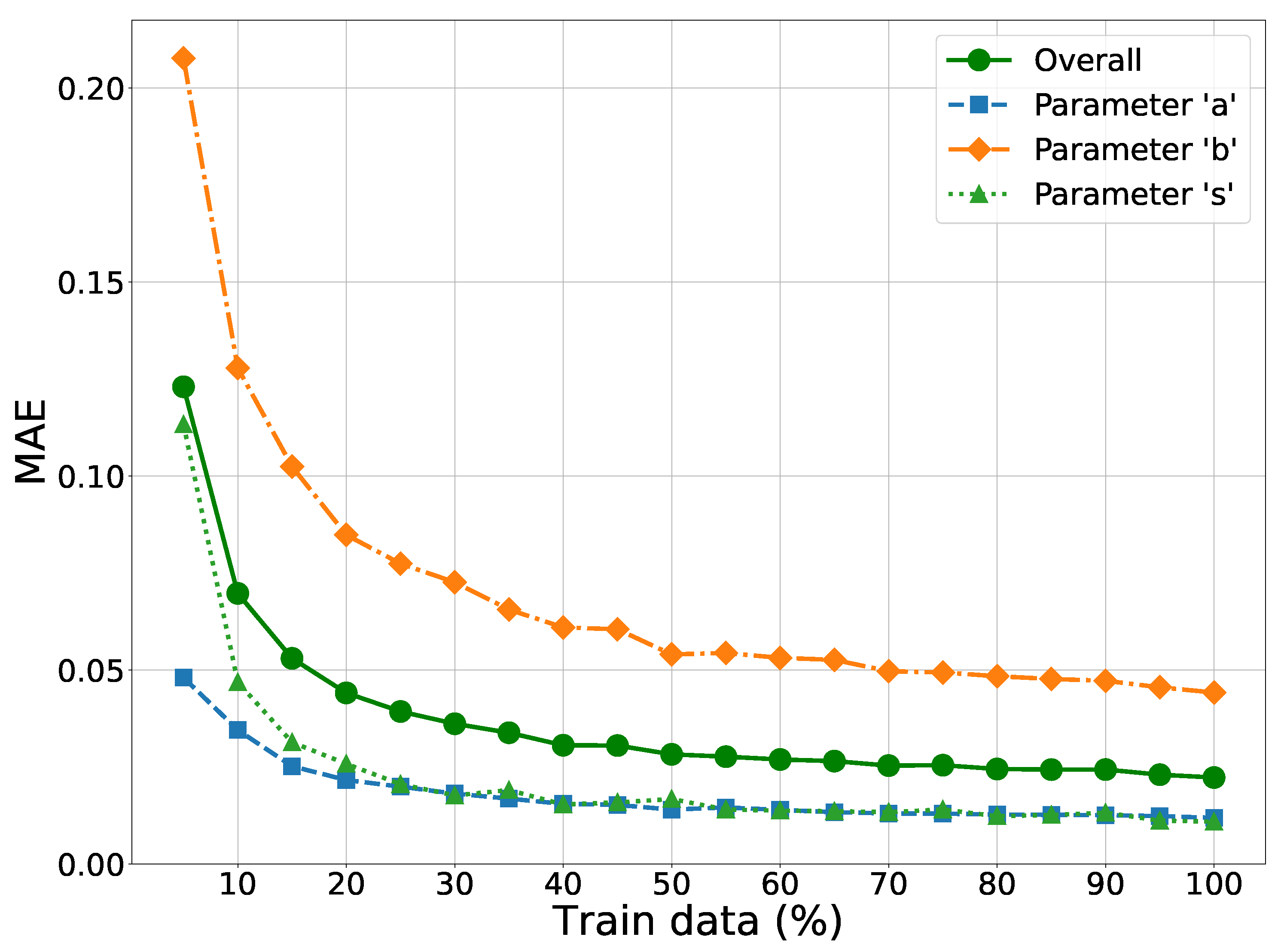
Figure 10.
Trends in MAE as more component signals are added to the composite signal.
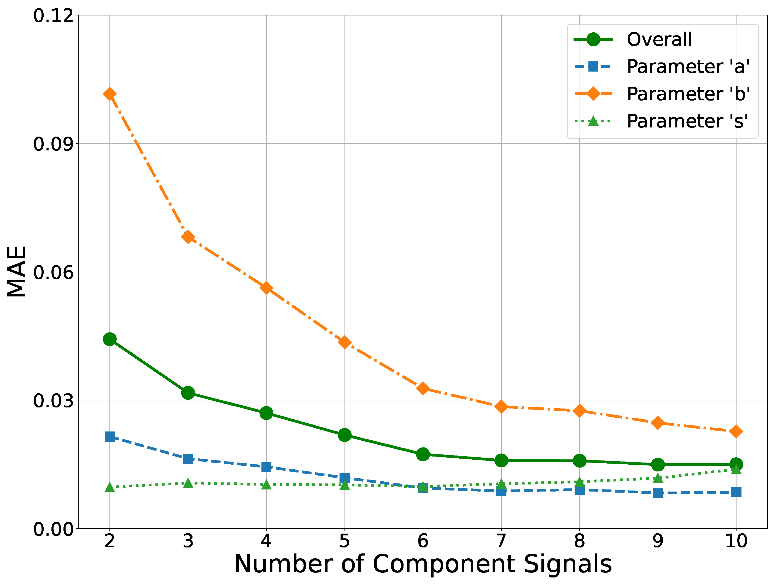
Figure 11.
Trends in score as more component signals are added to the composite signal.
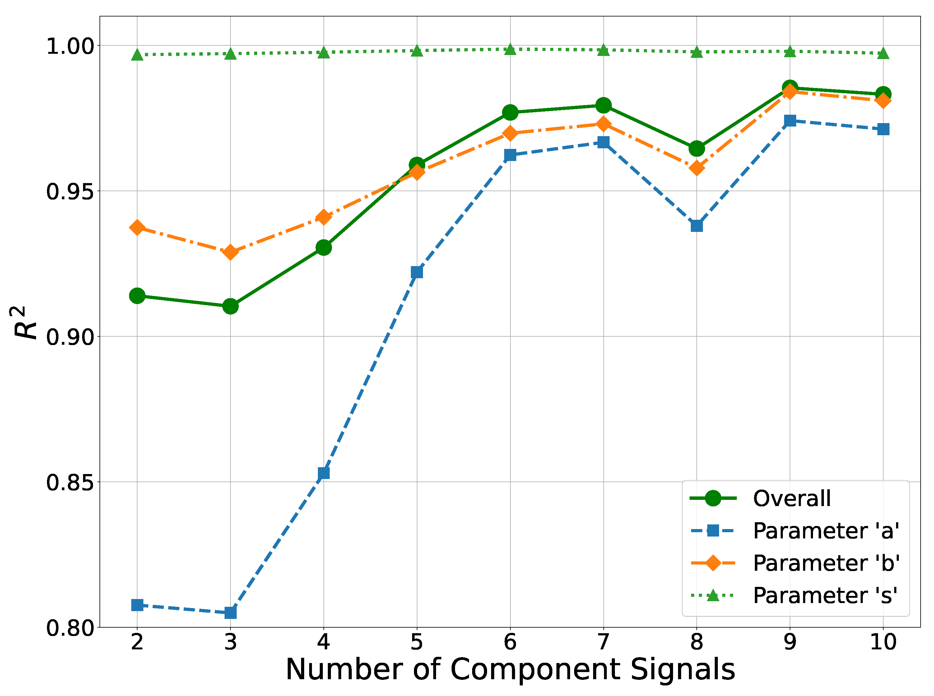
Figure 12.
score comparison for S-DNN and DNN.
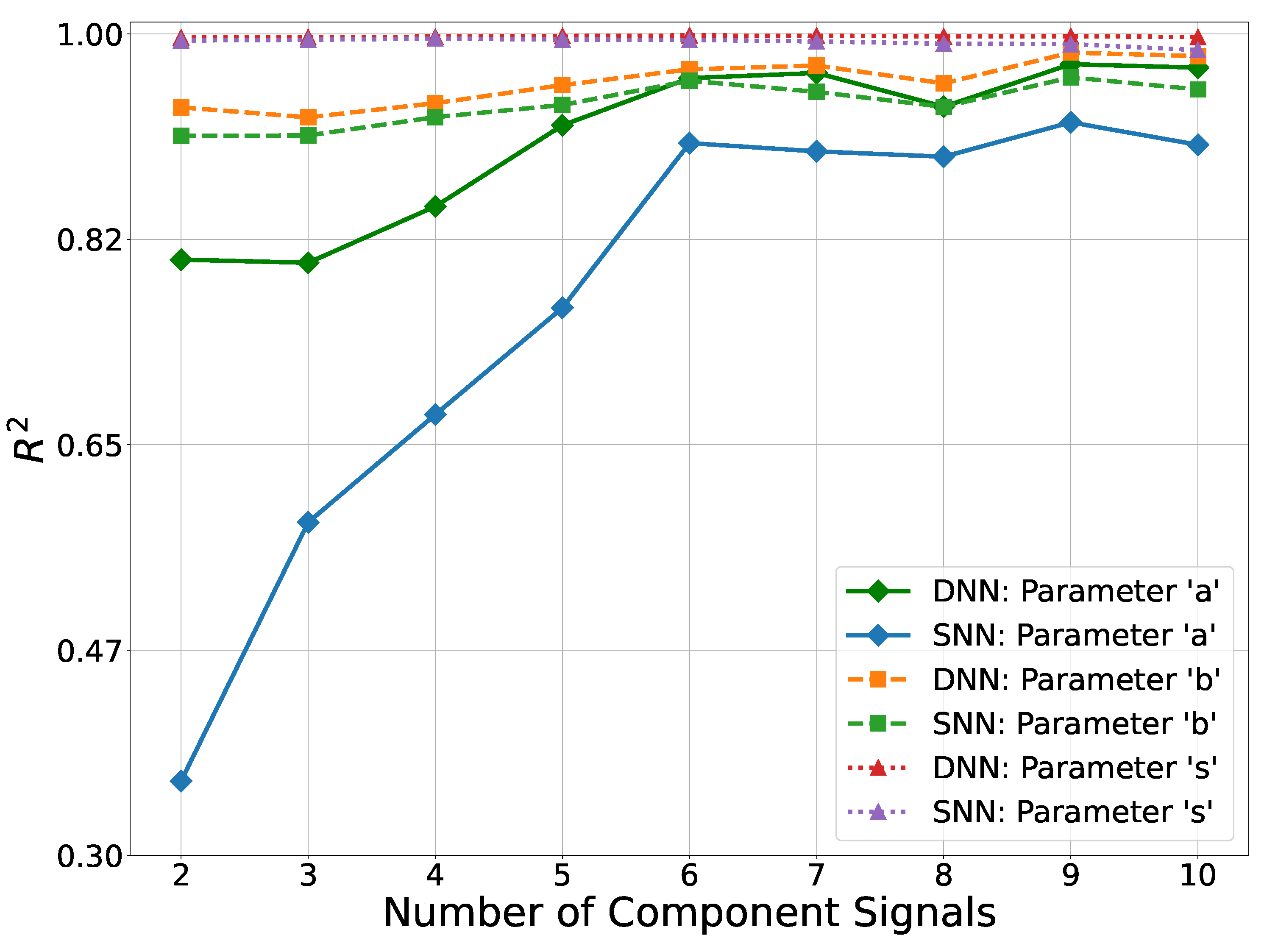
Figure 13.
CDF of the combined signal estimated using the DNN.
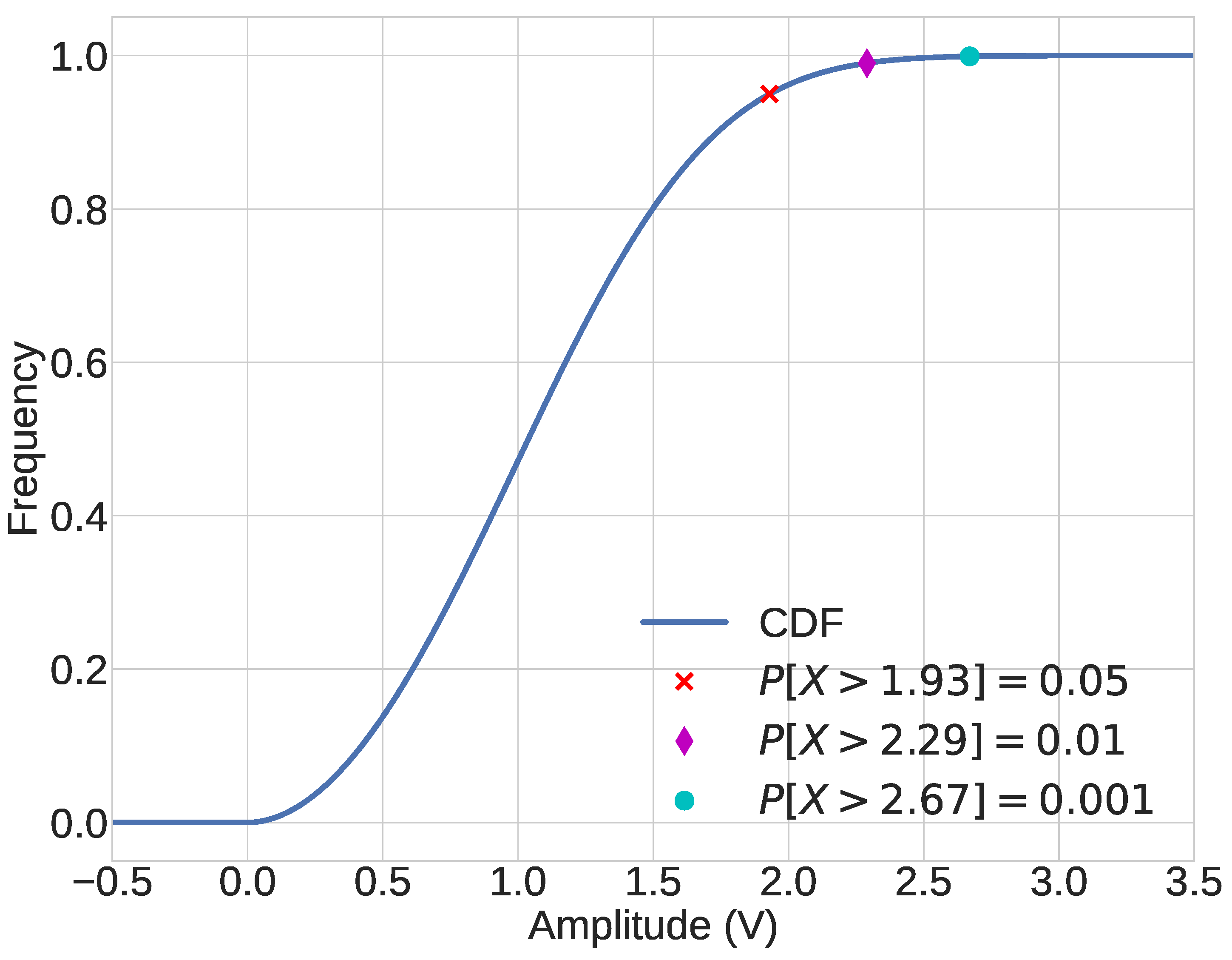

Table 1.
Range of parameters used for generating a combined signal.
| Parameter | Range |
|---|---|
| Modulation Order | |
| Data Rate | kbps |
| Power Level | dBm |
| Normalized Carrier Frequency | kHz |
Table 2.
SSE and KL-Divergence scores for the four distributions fitted to composite signals.
| Distribution | RSS | KL Divergence Score |
|---|---|---|
| Beta | 0.2637±0.3544 | 0.0020±0.0018 |
| Chi | 0.5200±0.6494 | 0.0065±0.0047 |
| Generalized Gamma | 0.0922±0.2189 | 0.0007±0.0009 |
| Rice | 0.2342±0.4192 | 0.0025±0.0031 |
Table 3.
, explained variance, MAE, and MSE performance scores obtained by the proposed DNN.
| Parameter | Explained Variance |
MAE | MSE | |
|---|---|---|---|---|
| a | 0.9358 | 0.9358 | 0.0119 | 0.0008 |
| b | 0.9664 | 0.9664 | 0.0442 | 0.0133 |
| s | 0.9985 | 0.9985 | 0.0109 | 0.0003 |
| Overall | 0.9669 | 0.9669 | 0.0223 | 0.0048 |
Table 4.
Normalized SHAP values calculated for the hold-out test set using the DNN.
| Parameter | Feature Groups (%) | ||||
| Modulation Order |
Data Rate | Power Level |
Normalized Carrier Frequency |
Number of Component Signals |
|
| a | 42.55 | 1.57 | 46.67 | 1.80 | 7.40 |
| b | 49.94 | 0.68 | 39.35 | 0.75 | 9.28 |
| s | 38.96 | 0.12 | 48.87 | 0.11 | 11.95 |
| Overall | 44.42 | 0.63 | 44.30 | 0.70 | 9.95 |
Table 5.
Training time and number of FLOPs for the DNN and S-DNN models.
| Model | Training Time (s) | FLOPs |
|---|---|---|
| DNN | 596 | 459548 |
| S-DNN | 407 | 17096 |
Table 6.
Comparison of scores obtained using different multi-output regression techniques.
| Method | a | b | s | Overall |
|---|---|---|---|---|
| LR | 0.4926 | 0.4484 | 0.6994 | 0.5468 |
| K-NR | 0.4795 | 0.5297 | 0.4447 | 0.4846 |
| DTR | 0.5578 | 0.7218 | 0.9400 | 0.7398 |
| RFR | 0.7651 | 0.8527 | 0.9745 | 0.8641 |
| GBRT | 0.8381 | 0.8982 | 0.9928 | 0.9097 |
| SVR | 0.5908 | 0.6814 | 0.9142 | 0.7288 |
| S-DNN | 0.8311 | 0.9548 | 0.9952 | 0.9270 |
| DNN | 0.9358 | 0.9664 | 0.9985 | 0.9669 |
Table 7.
Features of six component signals used to generate a composite signal.
| Modulation Order |
Data rate (bps) |
Power level (dBm) |
Carrier frequency (kHz) |
|---|---|---|---|
| 4 | 1544 | -7.59 | 17 |
| 128 | 3906 | -0.05 | 23 |
| 32 | 1707 | -17.39 | 31 |
| 4 | 7670 | -9.25 | -33 |
| 256 | 2846 | -11.29 | 34 |
| 128 | 2639 | -23.92 | 6 |
Disclaimer/Publisher’s Note: The statements, opinions and data contained in all publications are solely those of the individual author(s) and contributor(s) and not of MDPI and/or the editor(s). MDPI and/or the editor(s) disclaim responsibility for any injury to people or property resulting from any ideas, methods, instructions or products referred to in the content. |
© 2024 by the authors. Licensee MDPI, Basel, Switzerland. This article is an open access article distributed under the terms and conditions of the Creative Commons Attribution (CC BY) license (http://creativecommons.org/licenses/by/4.0/).
Copyright: This open access article is published under a Creative Commons CC BY 4.0 license, which permit the free download, distribution, and reuse, provided that the author and preprint are cited in any reuse.


