
Submitted:
05 December 2024
Posted:
06 December 2024
You are already at the latest version
Abstract
This paper presents a multimodal sentiment analysis system for analyzing and recognizing pain sentiments for the Internet of Things (IoT) Healthcare framework. This multimodal sentiment analysis system will analyze both facial patterns and speech-audio recordings to analyze human pain intensities. The implementation of the proposed system is divided into four components. The first component is to detect the facial region from the given image sequences of a video. Detecting facial regions is crucial based on the identified textual facial patterns. The second phase extracts discriminant and divergent features from the detected facial region using deep-learning techniques based on building convolutional neural network architectures, followed by improving fine-tuning parameters with transfer learning of some optimized models and fusion techniques. In the third phase, the speech-audio recordings are analyzed by extracting some divergent and valuable features, which undergo deep learning-based approaches to generate more divergent features. The performances reported due to image-based and audio-based pain sentiment analysis systems are fused at the fourth component to enhance the performance of the proposed multimodal sentiment analysis system, which is eligible to predict the different pain intensities, such as `High-Pain’, `Mild-Pain’, and `No-Pain’, that appeared on the facial pattern or the speech-audio recording of a person when they feel pain. Three standard image-based databases, such as 2D Face-pain-set, UNBC-McMaster shoulder pain, and BioVid Heat Pain databases, and one audio-based Variably Intense Vocalizations of Affect and Emotion Corpus (VIVAE) database, have been employed to test the proposed system. The performance of the image-based pain sentiment analysis system using a 2D Face-pain-set (2-class problem) is 76.23% accuracy, using the UNBC-McMaster shoulder pain database (3-class problem), 84.27% accuracy, and for BioVid Heat Pain database (5-class problem) 38.04% is obtained. Similarly, for the proposed audio-based pain sentiment analysis system, the highest performance is 97.56% for (50-50%) and 98.32% for (75-25%) Training-testing samples using the VIVAE database. The performance of the proposed system has been compared with some state-of-the-art methods that show its superiority. Finally, by fusing the decisions obtained due to image-based and audio-based deep learning models, the achieved performance is 99.31% for 2-class, 99.54% for 3-class, and 87.41% for 5-class obtained for the proposed multimodal pain sentiment analysis system.
Keywords:
IoT
; Sentiment Analysis
; Pain Recognition
; Multimodal
; CNN
; Audio
; Fusion
1. Introduction
In recent years, modern security systems have undergone significant transformation due to the revolutionary technology of the Internet of Things (IoT) [1]. IoT-enabled analytics and automation systems, which rely on software, sensors, and electronic devices, collect and transmit data over the Internet without requiring human intervention. Wireless networks powered by these advanced systems improve security and operational efficiency across various sectors, including healthcare, business, retail, military, and transportation. In healthcare, IoT plays a crucial role in automating patient monitoring and nurse call systems. For example, patient monitoring systems process data from smart devices such as thermometers, ECGs, pulse oximeters, and sphygmomanometers to predict health conditions and alert medical staff to initiate appropriate treatments. Building on these advancements, this study proposes a multimodal pain sentiment analysis system for remote patient monitoring, utilizing IoT-enabled medical sensors [2].
Multimodal sentiment analysis systems combine data from multiple sources: text, audio, and videos to assess sentiment. These are used to analyze customer opinions, feedback, and experiences. For example, suppose a customer surveys their experience with a product or service. In that case, a sentiment analysis system can analyze the customer’s words, tone of voice, facial expressions, and body language to determine the customer’s sentiment. The system can then categorize the sentiment as positive, negative, or neutral. In addition, the system can analyze the customer’s emotions, such as happiness, anger, and frustration. These emotions allow companies to gain more insights into customer sentiment and make informed decisions on improving their products and services. Here, multimodal pain sentiment analysis is extracting sentiment from a combination of textual and non-textual data sources related to pain. The healthcare framework encompasses medical professionals, hospitals, doctors, nurses, external patient clinics, clinical tests, telemedicine, medical devices, and machinery, as well as health insurance services [3]. Recent advancements in technology have significantly enhanced healthcare by introducing electronic and mobile-based health facilities. Mobile health (m-health) systems now provide patients with daily health support, enabling continuous monitoring and assistance [3]. These electronic healthcare systems utilize speech recognition, gesture movement, voice, and facial expression analysis to remotely assess patients’ health status. Gesture-based interaction and identification have become increasingly important in human-computer interaction (HCI), making e-healthcare systems more intuitive and accessible for doctors and nurses [4]. The proposed sentiment analysis system enriches these e-healthcare solutions, offering more cost-effective and efficient healthcare services. Furthermore, essential requirements such as authenticity, accessibility, security, advanced tools, and privacy have been carefully integrated into the system to ensure its reliability and effectiveness.
In recent years, computer usage has had a hugely significant impact since its advent. Web surfing, watching videos, playing games, online teaching and examination, e-commerce, and storing and retrieving data are some activities involving computer usage. As a result, Human-Computer Interaction (HCI) has grown as one of the most exciting domains in the field of research [5]. Thus, HCI is categorized as the live research areas [6]. Web services control various cloud-based devices as a platform of the Internet of Things (IoT) coming into the scenario along with HCI. In the last few years, IoT has earned immense popularity. The IoT-based devices are applicable in smart homes, traffic congestion control, and automatic driving. Along with these applications, the IoT also works with Artificial Intelligence (AI) in the healthcare infrastructure. The healthcare industry is considered a significant sector from the employment point of view, revenue, and health-associated convenience, and it contributes to a healthy civilization in smart cities. For patients who are non-verbal, the American Society provides an example of how to estimate pain emotion. The description shows a hierarchical structure for pain estimation, considering facial representation-dependent pain estimate as a legitimate method. Payen et al. [7] concluded that a pain valuator-based facial expression could be used for seriously ill, unflappable patients. A pain estimation analysis on aged patients with substantial mental sickness and due to growing mental illness, they are not able to communicate verbally, so the facial expressions are proper to assess the appearance of the pain of those particular patients. A pain valuator-based facial expression could be employed for highly ill, unflappable patients, according to Payen et al. [7]. An analysis of facial expressions in elderly individuals with severe mental disease is appropriate for estimating their level of discomfort because these patients are unable to express their feelings orally due to their worsening mental illness. McGuire and colleagues [8] came to the conclusion that individuals in the non-intellectual population may not recognize their discomfort or receive adequate treatment, mainly if they are unable to communicate their annoyance effectively.
A strong correlation exists between behavioral responses—such as grimacing, closing eyelids, and wincing—and procedural pain, as shown in studies involving patients [9]. Facial expressions, according to [10], effectively convey unpleasant emotions, making them essential indicators for assessing pain. Sentiment analysis systems in real-world applications remotely detect and interpret patients’ facial expressions to determine emotional states [3]. Pain assessment in clinical settings plays a crucial role in delivering appropriate care and evaluating its effectiveness [11]. The gold standard for pain reporting often involves patient self-reports using verbal numerical scales and visual analogue scales [12]. Certain vulnerable groups—such as those who are physiologically immobile, terminally ill [8], critically ill but coherent [7], experiencing psychological distress [13], or suffering from cancers affecting the neck, head, or brain require reliable technological support to provide consistent pain alerts, alleviating the burden on healthcare professionals. Other sentiment analysis systems have been developed for conditions like Parkinson’s disease, depression, intent analysis, facial emotion recognition, and contextual semantic search. These systems analyze text, image, and video data using deep learning techniques to classify emotions and identify patterns. The primary contributions of this work are outlined as follows:
- Deep learning-based frameworks utilizing handcrafted features are employed in the proposed audio-based pain sentiment analysis system.
- Several top-down deep learning frameworks are developed using Convolutional Neural Network (CNN) architectures to extract discriminative features from facial regions for improved feature representation.
- Performance enhancements are achieved through various experiments, including batch vs. epoch comparisons, data augmentation, progressive image resizing, hyperparameter tuning, and transfer learning with pre-trained deep models.
- Post-classification fusion techniques are applied to improve system accuracy. Classification scores from different deep learning models are combined to reduce susceptibility to challenges such as variations in age, pose, lighting conditions, and noisy artifacts.
- The proposed system’s applications can be extended to detect mental health conditions such as stress, anxiety, and depression, contributing to treatment assessment within a smart healthcare framework.
- Finally, a multimodal pain sentiment analysis system is constructed by fusing classification scores from both image-based and audio-based sentiment analysis systems.
2. Related Work
Numerous automatic techniques for identifying pain are insufficiently proficient in identifying pain based on facial representations. In the field of pain recognition systems from facial expression, some well-known feature extraction techniques, such as Active Appearance Models and Active Shape Model [14], Local Binary Pattern (LBP) [15], and Gabor wavelets [16], are used. It has been noted that the approaches now in use are related to facial representation-based pain detection. Specific techniques rely on deep learning, whereas others are focused on non-deep learning [17]. In recent years, significant progress has been made in this particular field of study. Regarding categorization, it has been noted that the retrieved face features [18] influence classification. A few popular feature extraction approaches perform this feature extraction task. The classification tasks are carried out using popular supervised machine learning techniques such as K-Nearest Neighbour [19], Support Vector Machine [20], and Logistic Regression [21].
A method for identifying acoustic pain detection in newborns based on audio features has been proposed in [22]. To explore the relationship between subjective pain reports and measurable biosignals in human speech, prosody was developed by Oshrat et al. [23]. In [24], an automatic evaluation system for pain based on paralinguistic speech was introduced, aiming to improve the objectivity and accuracy of pain diagnosis. A multimodal pain intensity recognition system using both audio and video channels was presented in [25]. Hossain [26] developed a multimodal sentiment analysis system for assessing patient states within a healthcare framework, using speech and facial expressions. Zeng et al. [27] conducted a psychological perspective survey on human emotion perception through audio, visual, and spontaneous expressions. Finally, Hong et al. [28] explored an improved method for automatic pain level recognition, incorporating the pain site as an auxiliary task.
In computer vision, features extracted by different CNN frameworks are utilized for different purposes like emotion recognition, object identification, etc. It has also been noticed that CNN dragged features perform better than handwrought features. In the last few years, growth in deep learning-based research activity has been found, and the outcome of this research activity has become the prominent solution to various cutting-edge problems. The classification of pain using the CNN framework was achieved in [29]. The proposed sentiment analysis system also leverages the high performance of CNN models, incorporating frameworks like GoogleNet [30] and AlexNet [31]. Liu et al. [32] introduced a hybrid neural network model combining CNN and BiLSTM to analyze emotions. A comparative study on sentiment analysis using bio-inspired algorithms was published by Yadav and Vishwakarma [33]. In [34], Hermawan et al. applied the concept of "Triplet Loss for Pain Detection" to classify pain based on different facial expressions. Haque et al. [35] proposed a two-part method, where the first part uses a 2D-CNN architecture to extract frame-wise features for pain recognition, and the second part employs Long Short-Term Memory (LSTM) to estimate temporal relations among the frames for sequence-level pain recognition. Menchetti et al. developed a pain detection system using two-stage deep learning networks: the first stage uses a Deep Neural Network (DNN) to extract facial landmarks, while the second stage employs a Convolutional Neural Network (CNN) to detect various Action Units [36]. Bandar et al. [37] proposed a feature learning-based classification method for pain detection.
Algorithms based on deep learning can enlighten internal dimmed patterns in complex datasets, which plays a vital role in feature extraction and classification [31]. Dashtipur et al. proposed a Multimodal Framework based on context awareness on Persian Sentiment Analysis [38]. Based on the movie review comments on emotion analysis, Sagum et al.[39] have proposed a sentiment measurement technique. Rustam et al. [40] compared the performances of various supervised machine-learning techniques based on Sentiment Analysis of COVID-19 tweets. The pain or anguish experienced when exposed to sound is called acoustic or auditory pain. This discomfort may appear in some ways, such as (i) Hyperacusis, An increased sensitivity to common environmental noises that can cause pain or discomfort even at low decibel levels; (ii) Phonophobia, Severe dread of loud noises or avoidance of them; frequently coupled with physical discomfort and anxiety; (iii) Tinnitus: This condition causes ringing, buzzing, or other phantom noises to be perceived in the ears; however, it is not always uncomfortable [41]. It has also been demonstrated that the acoustic elements of music, such as rhythm, speed, and harmony, will establish the connection between pain relief and music therapy.
Ghazal et al. [42] introduced a Principal Component Analysis (PCA) method to reduce the dataset and extract the most significant facial features, followed by the application of a CNN for face recognition. In their survey, Rasha M. et al. [43] identified and reviewed various pain detection methods, including multitask neural networks, CNN-LSTMs, and cumulative attributes. Additionally, they proposed a method for comparing feature extraction techniques, such as Skin Conductance Response (SCR) and Skin Conductance Level (SCL), to extract various features like root mean square, mean value of local maxima-minima, and mean absolute value for pain detection [44]. Patrick et al. [45] introduced a pain detection method that incorporated both Uni-Modal and Multi-Modal concepts. Eshan et al. [46] compared a Random Forest classifier using Facial Activity Descriptors with the performance of a deep learning-based approach for pain detection. Kornprom et al. [47] proposed a pain estimation method along with a pain intensity metric, using tools such as the Visual Analog Scale, Observer Rating Scale, Affective Motivational Scale, and Sensory Scale. Leila et al. [48] developed a specific model for automatic pain detection using the VGG-Face model on the UNBC dataset. Jiang et al. [49] conducted experiments employing the GLA-CNN approach for pain detection. Finally, Ehsan et al. [50] proposed a pain classification system using video data from the X-ITE dataset.
3. Proposed Methodology
This section outlines the implementation of the proposed pain sentiment analysis system. Facial expressions play a significant role in detecting pain sentiment, with the features of these expressions contributing to the identification of pain intensity. In cases where facial features are unavailable, audio-based sentiment features are utilized. Additionally, as facial expressions may vary from person to person due to the perception of pain, audio-based information can assist in determining the pain level. Therefore, combining both modalities enhances the performance of the proposed pain detection system. While several established pain detection algorithms exist, there is still room for improvement in pain recognition techniques. In the current landscape, cloud-dependent mobile applications that rely on streaming data and live video processing are gaining popularity. These applications typically consist of two components: the front-end, which runs on mobile devices, and the back-end, which operates in the cloud. The cloud provides enhanced data processing and computational capabilities. Our proposed method allows for the execution of complex applications on devices with existing resources and potential, optimizing performance. This section describes a sentiment analysis system for estimating pain intensity based on facial expressions. The research integrates cache and computing facilities to provide essential modules for an electronic healthcare system. The proposed system is divided into five key components for implementation, with the block diagram of the pain recognition system shown in Figure 1.
This block diagram of our proposed system shows that there will be a cloud network capable of storing some data. Various devices from outside the system will communicate through that network. Our database is also connected to the cloud network. Our database is mainly consisting of images, videos, and audio. Before classification, images are fetched from the database, preprocessed, and reshaped based on the algorithm. The core implementation of the proposed system is as follows: once the preprocessing is completed, the images are separated into training-testing segments and sent to two different architectures. These architectures are trained with the training images separately. Once the training is completed, the prediction model is obtained. The prepared prediction models generate scores corresponding to the input sample. Then, based on the score level fusion technique, the final decision is made regarding the outcome of the proposed system. The obtained prediction model is connected to the network so that the pain’s intensity can be predicted from external remote devices for the patients. The detailed implementation of the proposed system is elaborated on in the subsections below.
3.1. Audio-Based PSAS
In the digital world, audio-based media content is kept in the form of signal processing, where the dealing, processing, and manipulation of audio signals are performed for various applications such as speaker recognition, gender classification, age classification, disease detection, entertainment, and health care. Converting analogue signals to digital signals in audio files is much more challenging among the several types of media content, such as texts, images, videos, and audio. The chances of unwanted noise introduction and unbalanced time-frequency distribution make the audio-based recognition systems much more challenging. In this work, an audio-based speaker’s sentiment analysis has been performed to detect the intensity levels of their body-part pain sentiments. The purpose of an audio noise reduction system is to remove noise from audio signals, such as speech. There are two types of these systems: complementary and non-complementary. Before properly recording the audio stream, complementary noise reduction entails compressing it. Conversely, single-ended type, or non-complementary, noise reduction works well for lowering noise levels [51]. Digital and analogue devices are vulnerable to noise because of specific characteristics. It is possible to extract different aspects more precisely when noise is removed from audio signals. In this work, we have utilized filtered audio signals to extract features for the audio-based pain sentiment analysis system (PSAS). Here, identifying pain sentiment levels is based on analyzing the types of emotions a person has during human-computer-based interaction in the healthcare system. Fortunately, facial expressions are analyzed or recognized in image or video-based emotion recognition. Still, in real-time scenarios, video-based media might record the vocal emotions of a patient in the online healthcare framework. Then, there will be the requirement for audio-based emotion recognition systems. Here, the feature representation using the deep learning-based approach for audio-based classification has been demonstrated in Figure 2.
This work considers a speaker’s audio recording for the audio-based pain sentiment analysis. The audio data is in the form of a waveform audio file containing a byte sequence representing some audio signals over time. Hence, analyzing these sequences of bytes in terms of numeric feature representation, some feature extraction techniques are employed for feature computation from the waveform audio files. These feature extraction techniques are described as follows:
- Statistical audio features: Here, the audio signal initially undergoes a frequency domain signal analysis using fast Fourier transformation (FFT) [52]. Then, the computed frequencies are used to calculate descriptive statistics such as mean, median, standard deviations, quartiles, and kurtosis. Further, the magnitude of derived frequency components is used to compute Energy, and the amplitude is used to calculate Root Mean Square Energy.
- Mel Frequency Cepstral Coefficients (MFCC): This is a well-known audio-based feature computation technique [53] where the derived frequency components from FFT undergo to compute the logarithm of the amplitude spectrum. Then, the Mel scale is introduced to the logarithm of the amplitude spectrum, discrete cosine transformations (DCT) are applied on the Mel scale, and finally, 2-13 DCT coefficients are kept. The rest are discarded during feature computations.
- Spectral Features: Various spectral features like spectral contrast, spectral centroid, and spectral bandwidth are analyzed from the audio files. These spectral features [54] are related to the spectrogram of that audio files. The spectrogram represents the frequency intensities over time. It is measured from the squared magnitude of the Short-Time Fourier Transform (STFT) [55], which is obtained by computing FFT over successive signal frames.
So, using these above feature extraction techniques, -dimensional statistical features (), -dimensional MFCC features (), and -dimensional spectral features () are extracted from each speech-audio. Then, these feature vectors are concatenated such that . Now, , , undergoes to the proposed deep-learning based feature representation followed by classification for speech-audios. During feature representation, d-dimensional feature vector is transformed to 512-dimensional features, then 256 to 128-dimensional features. Finally, during classifications, maps into 3-class audio-pain problems. The list of parameters required for the audio-based deep learning technique is demonstrated in Table 1.
3.2. Image-Based PSAS
During the image acquisition phase, noise is often introduced, which reduces the textural information and detail of facial patterns essential for pain sentiment recognition. This noise can negatively impact the experiment’s accuracy. In the preprocessing phase, a color image is processed to extract the facial region for pain emotion detection. This research employs a tree-structured part model [56], which is effective for various face poses. For frontal faces, the method identifies a total of sixty-eight landmark points, while for profile faces, it identifies thirty-nine. Once the facial landmarks are detected, the extracted facial portion undergoes an image normalization process. Bilinear image interpolation is applied to normalize the extracted face portion to an image size of . After normalization, feature computation tasks are performed. Several deep learning approaches are utilized to extract valuable and discriminating features. Different deep learning architectures are applied individually to the same dataset, and the results from both architectures are fused to make the final decision in the proposed system. The process of detecting the facial region for the proposed pain identification system is illustrated in Figure 3.
3.3. Image-Based Feature Representation Using Proposed Deep Learning Architectures
Visual feature extraction provides a reliable and consistent way to distinguish between various objects. In tasks such as emotion classification and facial expression identification, effective feature representation plays a critical role [57]. It is not feasible to directly classify facial emotion-based pain levels using raw, unprocessed features. In this work, strong and efficient local-to-global feature representation schemes are applied for both feature synthesis and representation. Convolutional Neural Network (CNN) architectures have successfully extracted a range of distinct features from images and videos through various deep learning techniques [58]. In CNNs, different kernels process images using mixed convolution operations [59]. After convolution, the network employs a pooling technique with weight sharing to optimize network training parameters. While statistical and structural-based methods in computer vision exist, state-of-the-art CNN feature representation techniques are highly effective for facial expression-based pain sentiment analysis. These general CNN features provide superior performance by handling articulation and occlusion in face images captured in unconstrained settings [58]. They enhance performance by overcoming the challenges of occlusion and articulation in face images taken in uncontrolled environments. The proposed system’s performance includes a sentiment analysis component that analyzes facial expressions, balancing deep learning features with variables that influence the effectiveness of these features.
The proposed feature representation schemes describe the two primary functions of the CNN baseline model: feature extraction and classification. The architecture of the proposed CNN models consists of seven to eight deep image perturbation layers. These layers utilize the ReLU activation function during convolution operations, followed by max-pooling and batch normalization to extract features. The extracted feature maps are then passed through two fully connected flattened layers for classification tasks. The performance of the proposed CNN model has been enhanced through progressive image resizing techniques, which add new levels to the model. These techniques help reduce overfitting and address imbalanced data issues, while also minimizing the computational resources required. Proper learning of weights is crucial, as only the pre-trained weights from the previous layers are utilized. In addition, techniques such as activation functions, batch normalization, image augmentation, regularization methods (e.g., mix-up optimizer and label smoothing), and other regularization techniques are employed to further optimize the model. At the core of the CNN architecture is the convolution operation, which plays a fundamental role in feature extraction [57]. The convolution operation involves combining two functions to produce a third, where features are extracted from the images. A sized kernel or filter is used to perform the convolution over the input image, producing feature maps. This process involves sliding the filter over the image and applying non-linearity, followed by matrix multiplication at each location and adding the result to the feature map. To further enhance the performance of the proposed recognition system, fine-tuning of parameters is carried out, and score-based fusion techniques are applied for improved results.
The Convolution Neural Network (CNN) architectures based on deep learning are being used here [30] to perform feature learning and classify facial region images into two or three pain-level class problems. The performance of an emotion recognition system based on facial expressions is severely compromised by over-fitting, which leads to expression alterations such as changes in head pose, age, identity, and illumination. The proposed approach emphasizes these issues and restores the CNN model’s computational complexity. The shape and texture information can be extracted from the images with the hybrid nature of the proposed architectures. The recommended system’s feature description uses textual details and shapes to give both geometrical and appearance features. The primary drawback of the CNN model, which is thought to be significant computation power loss, can be mitigated by using Graphical Processing Units. The Graphical Processing Units are primarily designed to handle a high volume of computation, including countless levels of representation and concepts for handling transfer learning, pretraining, data patterns, and techniques for fine-tuning CNN models. In this work, during training the proposed architectures, some heavy databases are used to train the architectures by adjusting the weights of the network based on the number of defined pain-class problems. So, this research proposes two Convolutional Neural Network (CNN) architectures, such as and . The respective trained models generated from these architectures are , and . For a better understanding and transparency regarding the models, the specifics of these architectures with their use of input-output hidden layers, convoluted image output shape, and parameters produced at each layer are further described. These are shown in Figure 4 and Figure 5, respectively. Similarly, Table 2 and Table 3 describe the list of parameters required for training these architectures.
The convolution operation is the core operator in this network and serves as the fundamental structural block of the CNN architecture. This operation is responsible for extracting features from images. To apply the convolution operation to the input image F, a filter or kernel of size is used to generate feature maps. The convolution operation is performed by sliding the filter across the input image I, applying non-linearity at each location. Element-wise matrix multiplication is carried out, and the results are aggregated to form a feature map element corresponding to the center of the mask pattern. To improve the performance of the proposed CNN architectures, fine-tuning of parameters is applied. Max-pooling is used to calculate the maximum value for strips of the feature map, resulting in a down-sampled feature map. The max-pool layer serves multiple purposes: (i) it ensures uniform translation, (ii) reduces computational overheads, and (iii) enhances the generation of discriminative features from the input image I. The architecture comprises six convolution blocks. Each block contains a series of layers, including a Convolutional layer, a MaxPooling layer, a BatchNormalization layer, and a Dropout layer. These layers are followed by a flattened layer. The network also includes three fully connected blocks, each with two Dense layers and a Dropout layer. The final output layer consists of a Dense layer. During compilation, the ’Adam’ optimizer is employed for optimization.
- Convolutional Layer: The convolutional layer generates feature maps Z by applying a kernel or mask of size to perform a convolution operation on the input image I. During this process, the kernel slides across the input image F, associating each region of the image with a non-linear activation function. At each location, element-wise matrix multiplication is performed, and the resulting data is summed to form an element in the feature map corresponding to the central region of the mask pattern. The convolutional layers with N (e.g., 32, 64, 128, 256, 512, 1024, etc.) are implemented as , where M denotes the number of convolutional layers in the CNN architecture, with , represents the weights of the M-th convolutional layer, * indicates the convolution operation, and corresponds to the biases of the M-th convolutional layer.
- Max-Pooling Layer: The max-pooling operation contributes to fine-tuning the parameters of the proposed CNN architecture, enhancing its performance. This operation involves calculating the maximum values within segments of the feature map, followed by the creation of down-sampled feature maps. Max-pooling offers several advantages, including uniform translation, reduced computational overhead, and improved selection of discriminative features from the input image I. If represents the output feature map from the input image F, the max-pooling operation is applied as .
- Batch Normalization Layer: Batch normalization acts as a controller, enabling the model to utilize higher learning rates, which are beneficial for performing image classification tasks [60]. Specifically, it stabilizes gradients across the network by mitigating the effects of parameter scales or initial values.
- Dropout Layer: In architectures, the dropout layer serves as a regularization technique to prevent overfitting. It compels the network to develop more robust and generalized features during training by randomly deactivating a subset of neurons. By reducing the dependency between neurons, the dropout layer enhances model performance and generalization on unseen inputs, leading to more efficient and reliable architectures.
- Flatten Layer: In , the flatten layer acts as a bridge between the convolutional and fully connected layers. It transforms the multi-dimensional feature maps into a one-dimensional vector, making them compatible with the subsequent fully connected layers. By converting complex spatial data into a linear format, the flatten layer enables the network to capture higher-level patterns and relationships, which are essential for tasks such as classification and decision-making.
- Fully Connected Layer: In every architecture, the fully connected layers are essential for performing classification. They transform the complete feature maps into isolated vectors, which are then used to generate class scores. This classification process produces a final vector whose size is determined by the number of class labels. The weight values in the dense layer help establish the connection between the input and output layers. The input to this layer is the output of the flatten layer, denoted by F, and the output of the R-th fully connected layer is represented by . The fully connected layer also incorporates the dropout layer for regularization.
- Output Layer: The output layer is responsible for classification, and the Softmax activation function is employed for this purpose. It utilizes the fully connected layer once more. The final output of this layer is denoted by Y, and its input, which comes from the fully connected layer, is represented by . The output is given by the equation , where are the weights, and are the biases associated with this layer.
After training, the trained model is derived from the architecture. In the higher feature representation scheme, another architecture is proposed, which is composed of eight blocks, where each block is also composed of a convolution layer, max-pooling, batchNormalization, and dropout layers and, after that, three flatten layers. Each flatter layer comes after One dense layer, one batch normalization, the activation function "Relu," and one dropout layer. Lastly, this architecture contains the final dense layer. An Adam optimizer is used during the architecture compilation process. After training, the trained model is derived from the architecture. The performance of these and architectures are affected by several factors to improve not only the performance but also the efficacy of the derived model with better feature abstraction schemes for the proposed image-based pain sentiment analysis system.
(i) The scheme’s first factor is progressive image resizing (). The input layers in will continuously obtain the image as input data. Convolution operations, on the other hand, will be carried out by numerous masks or filter banks. Various convolved images, or feature maps, are obtained based on the specific filters [61]. Convolution operations will perform more as image size increases, and the network will need to perform enormous computations as the number of filters rises. The parameters in these filter sets will be considered as refined weights. In terms of max-pooling layers, the number of parameters in the network similarly affects this layer’s computational barrier. As a result, it has been found that when patterns are analyzed from multiple image resolutions, the models perform better regarding feature representation of images using deep learning techniques. Further analysis of hidden patterns in the feature maps is made possible by adding more layers to the architecture as image resolution increases. Motivated by these findings, we have implemented several multi-resolution facial image techniques using different CNN architectures and layers. During feature representations, in this work, two different image resolutions of the normalized facial region F have been considered for such that the is down-sampled to , and , whereas .
(ii) The second factor is , which pertains to the Transfer Learning and Fine Tuning effects that influence the performance of the proposed CNNs. Transfer learning enables further development of discriminant features required for the PSAS, which demands higher-order feature representation. In this process, certain layers and their corresponding parameters are frozen while others are retrained to reduce the computational load. Transfer learning allows a model trained for one problem to be effectively applied to other related problems. In our proposed model, we leverage a transfer learning technique that integrates convolutional neural network (CNN) deep learning. To address the same problem, the new model utilizes the collection of layers and weights from a pre-trained model. This approach helps reduce training time and minimizes generalization error.
(iii) The third factor, , involves the deployment of Fusion techniques. In this approach, the trained models generate features or scores, which are then transformed into other sets of features or scores based on their values. These fusion techniques are applied to combine the classification scores produced by the trained deep learning models, improving the performance of the Pain Sentiment Recognition System (PSRS). The fusion of test sample scores is performed using methods that fall under two categories: post-classification (b) and pre-classification (a) techniques. In this work, post-classification methods, such as Sum-of-score, Product-of-score, and Weighted-sum-of-score, are used, as the trained deep learning models are already employed. Consider two trained deep learning models, and , which solve an L-class problem and generate classification scores and for a test sample a. The fusion methods are applied as follows:
- (i) The Sum-of-score is defined as ,
- (ii) The Product-of-score is defined as ,
- (iii) The Weighted-sum-of-score is defined as ,
where and are the weights assigned to models and , respectively, such that . Experimentally, it has been observed that when the performance of exceeds that of , then , and vice versa.
4. Experiments
The proposed multimodal pain sentiment analysis system has been implemented using Python in this research. The implementation was conducted on a system equipped with an Intel Core i5 processor (3.20GHz) and 16GB of RAM, running the Windows 10 operating system. Several essential Python libraries were utilized during the implementation, including Keras [62] and Theano [63]. These packages facilitated the development of deep learning-based convolutional neural network (CNN) architectures and techniques, which are central to the proposed system. In this work, facial image regions were employed to extract critical information that aids in determining the pain-level intensity of individual subjects.
4.1. Databases Used
The proposed system has been evaluated using one audio-based dataset, the "Variably Intense Vocalizations of Affect and Emotion Corpus (VIVAE)" [64], and two image-based datasets: the UNBC-McMaster shoulder pain expression archive dataset [65] and the 2D Face Set database with pain expressions, known as D2 [66]. The UNBC-McMaster shoulder pain expression archive dataset consists of 129 participants (66 female and 63 male), all of whom experience shoulder pain identified by physiotherapists at a clinic. The videos in this dataset were recorded at McMaster University. Participants in this study were assumed to be suffering from conditions such as bone spur, tendinitis, rotator cuff injuries, bursitis, arthritis, impingement syndromes, subluxation, capsulitis, dislocation, all contributing to their shoulder pain. From these videos, images were extracted and labeled according to pain intensity, ranging from ’No pain’ to ’high-intensity pain’ classes. In this research, the images were categorized into two or five pain classes. For the 3-class problem, the following labels were used: Non-Aggressive (NAG) for No-pain (), Covertly Aggressive (CAG) for Low-pain (), and Overtly Aggressive (OAG) for High-pain (). Some image samples from the UNBC-McMaster dataset are shown in Figure 6, and the dataset’s description, including the 2-class and 3-class problems, is provided in Table 4. The second dataset used is the 2D Face Set Database with Pain Expression () [66], which contains 599 images from 13 women and 10 men. This dataset primarily involves a 2-class problem, with 298 images labeled as ’No-Pain’ () and the remaining 298 images labeled as ’Pain’ (). A description of this database is provided in Table 4, and several sample images from the 2DFPE database are shown in Figure 7.
The BioVid Heat Pain Database [67] is the third dataset used in this research, and it is based on video samples. The dataset consists of twenty videos per class and five distinct classes for each of the 87 subjects (persons). The five distinct data categories in the dataset are Part A through Part E, with Part A being selected for this work. From the list of 87 subjects, five subjects were chosen for Part A, with 50 videos considered for each subject. As there are five different classes for each subject, ten videos of each class were selected. In total, 250 videos were chosen, each lasting 5.5 seconds and containing 138 frames. The frames or images from each video were extracted and assigned one of five distinct labels, ranging from "No pain" to "extreme intensity pain." These labels correspond to the following pain intensity categories: baseline (), Intensity of ’Pain-Level 1’ (), Intensity of ’Pain-Level 2’ (), Intensity of ’Pain-Level 3’ (), and Intensity of ’Pain-Level 4’ (). Example images from the BioVid Heat Pain Database are shown in Figure 8. A description of the BioVid Heat Pain Dataset, including its correlation to image samples for specific pain classes, is provided in Table 4.
The fourth database is a speech audio database, the Variably Intense Vocalizations of Affect and Emotion Corpus (VIVAE) [64]. This VIVAE database is composed of audio files of non-speech emotion vocalizations of human beings. There are 1085 audio files in this database, while eleven speakers have participated in giving their speeches to this database. Each speaker expresses their fear, anger, surprise, pain, achievements, and sexual pleasure emotions. Each speaker’s emotion has been recorded into four intensities: ’ low’, `moderate’, `peak’, and `strong’. Since this work is related to detecting pain intensities among Non-Aggressive (NAG) (No-pain) (), Covertly Aggressive (CAG) (Low-pain) (), and Overtly Aggressive (OAG) (High-pain) () classes, so, for convenience, `low’, and `moderate’ are kept in NAG class, `peak’ in CAG class, `strong’ in OAG class. At the same time, all four emotions are categorized into these three classes based on their intensities. Hence, this database contains 530 audio of NAG, 272 audio of CAG, and 282 audio of OAG classes. So, different training-testing sets are employed during experiments to test the proposed system.
4.2. Results for Image-Based PSAS
There are two specific steps in the feature learning with the classification process of an image-based pain sentiment analysis system (PSAS): (i) image preprocessing and (ii) feature learning with classification. The facial region is extracted as the region of interest during this image preprocessing step. After that, the image size is changed to and for the normalized facial region . Then, the training dataset’s transformed facial images are subjected to the proposed CNN architectures (Figure 4) and (Figure 5), where the input image for the architecture is , and the input image for the architecture is . Activities such as feature computation and pain sentiment categorization are trained into the CNN architectures. The concentration on training the CNN architectures has been done to understand these architectures’ functions better. On the other hand, the trained model and go through to find out how well the system works with test samples. The architecture with a (50-50%) training-testing strategy is the starting point of the experiment. It is employed for the 2DFPE Database (2-class Pain levels) and UNBC Database (3-class Pain levels) databases.
-
experiments: This experiment is associated with parameter learning, which builds on batches and epochs and is fundamental to every CNN architecture. Both batch vs. epoch factors impact the architecture’s learning capacity when samples are trained inside the network. In any deep CNN model, one of the most critical tasks is to learn the weight parameters. As a result, this work has established a trade-off between 16 batches and 1500 epochs, enhancing the proposed pain sentiment analysis system’s (PSAS) performance. An experiment comparing batch and epoch for the proposed system is displayed in Figure 9 using the UNBC 2-class dataset, and it can be seen from Figure 9 that performance improves with batch size 16 and epoch variations ranging from 1000 to 1500.Here, in the , experiments are also performed to introduce multi-resolution facial images by utilizing progressive image resizing. The introduction of this scheme needs the use of multi-resolution image analysis in order to benefit from progressive image scaling, such that the image of two different sizes are trained via the and architectures. In comparison to the architecture performance, the offers the following benefits: (i) networks can be trained with images ranging from low to high resolution; (ii) hierarchical feature representations corresponding to each image can be obtained with improved texture pattern discrimination; and (iii) overfitting problems can be minimized. Figure 10 shows the multi-resolution image analysis performance for the proposed PSAS employing for 2DFPE Database (2-class Pain levels), UNBC Database (2-class Pain levels), UNBC Database (3-class Pain levels), and BioVid Heat Pain Dataset (5-class Pain levels) databases. From this figure, it has been observed that the derived model resolves the overfitting issue and improves the proposed system’s performance.
- experiments: This experiment is about measuring the effectiveness of introducing the Transfer-learning with fine-tuning of parameters when two new CNN models are being trained on the same domain of data (i.e., images). Fine-tuning refers to taking into account the weights of one proposed CNN architecture. It shortens the training period, which leads to better results. Transfer learning is a machine learning technique in which a model that is suggested for one job is utilized as a foundation for a different model on a different task. Different transfer learning methodologies have been applied here: (i) in the first approach, we used the refreshed models, i.e., we trained both CNN architectures and from scratch using the relevant image sizes; (ii) in the second approach, we used the retrained model of both architectures. We can see that CNN architectures perform better when employing these retrain models. Table 5 shows the CNN architectures’ performance. The accuracy and F1-score are the basis for the reported performances. The results in Table 5 indicate that Approach-1 improves PSAS performance.
- experiments: This experiment begins with the application of multiple Fusion techniques on the classification scores generated by the trained and architectures. Deep-learning features are utilized to obtain the classification results, and a post-classification approach is applied for fusion. The respective CNN models generate the classification scores, which are then subjected to the Weighted Sum-rule, Product-rule, and Sum-rule procedures for post-classification fusion. The fused performance of the proposed system, resulting from various combinations of fusion methods, is presented in Table 6. The fusion results demonstrate that the proposed system performs better with the Product-rule fusion approach, using both CNN architectures, compared to the Weighted Sum-rule, Sum-rule, and Product-rule techniques. The proposed system achieves an accuracy of 85.15% for the 2-Class UNBC, 83.79% for the 3-Class UNBC, and 77.41% for the 2-Class 2DFPE database. These performance results serve as a reference point in the section below.
-
Comparison with existing System for Image-based PSAS: The performance of the proposed system has been compared with several current state-of-the-art techniques across the 2-Class 2DFPE database, the 2-Class and 3-Class UNBC-McMaster shoulder pain databases, and the 5-Class BioVid Heat Pain database. Feature extraction for the local binary pattern (LBP) and Histogram of Oriented Gradient (HoG) procedures, as utilized in [68] and [69], has been employed. Each image’s feature representation approach uses a size of pixels, and the images are divided into nine separate blocks for both the LBP and HoG approaches. From each block, a 256-dimensional LBP feature vector [69] and an 81-dimensional HoG feature vector [68] are extracted, resulting in 648 HoG features and 2304 LBP features per image. For deep feature extraction, methods like ResNet50 [70], Inception-v3 [71], and VGG16 [72] were employed, with each using an image size of . Transfer learning techniques were applied, where each network was independently trained using samples from two or three class problems. Features were then extracted from the trained networks, and neural network-based classifiers were used for test sample classification. Competing approaches such as those by Lucey et al. [65], Anay et al. [73], and Werner et al. [74] were also implemented using the same image size of . The results for all these competing techniques were obtained using identical training and testing protocols as the proposed system. These results are summarized in Table 7, which demonstrates that the proposed system outperformed the competing techniques.Hence, Table 7 presents the performance comparison for the image-based sentiment analysis system using the 2-class and 3-class pain sentiment analysis system. All experiments were conducted under the same training and testing protocols. Quantitative comparisons were made between the proposed system’s two-class classification model (A) and the competing methods: Anay et al. [73] (B), HoG [68] (C), Inception-v3 [71] (D), LBP [69] (E), Lucey et al. [65] (F), ResNet50 [70] (G), VGG16 [72] (H), and Werner et al. [74] (I). The statistical comparison of the performances between the proposed system (A) and the competing methods ({B,C,D,E,F,G,H,I}) is shown in Table 8. A one-tailed t-test [75] was conducted using the t-statistic to analyze the results. The one-tailed test assumes two hypotheses: (i) H0 (Null-hypothesis): (indicating that the proposed system (A) performs on average less than or equal to the competing method’s performance); (ii) H1 (Alternative-hypothesis): (indicating that the proposed system (A) performs better on average than the competing methods). The null hypothesis is rejected if the p-value is less than 0.05, indicating that the proposed method (A) performs better than the competing methods. For the quantitative comparison, each test dataset for the employed databases was divided into two sets. For the database, there are 298 test image samples (Set-1: 149, Set-2: 149). For the UNBC (2-Class/3-Class) problem, there are 24,199 test samples (Set-1: 12,100, Set-2: 12,099). The performances of the proposed method and the competing methods were evaluated on these test sets. Table 8 shows the results of the quantitative comparisons for the employed databases. From this table, it is evident that in every comparison between the proposed system and the competing methods, the alternative hypothesis is accepted and the null hypothesis is rejected, confirming that the proposed method (A) outperforms the competing methods.
4.3. Results for Audio-Based PSAS
In the case of the audio-based pain sentiment analysis system (PSAS), the feature representation using the Deep learning-based approach (discussed in Section 3.5 (Figure 2)) has been employed. Here, the above-discussed audio-based features such as Statistical audio features, Mel Frequency Cepstral Coefficients (MFCC), and Spectral Features are employed, extracted from each speech-audio using Librosa [76] python package. This package is used for audio, speech, and music analysis. Here, 11 statistical features, 128 MFCC features, and 224 spectra features are extracted using this package. During experimentations, each set of these features and a combination of these features are experimented with individually correspond to machine learning classifiers such as Logistic regression, K-nearest neighbour, decision tree, and support vector machine concerning 50-50% and 75-25% training-testing sets. Each individual and combined feature set is employed for the deep learning-based feature representation scheme. Table 9 demonstrates the performance of the proposed audio-based pain sentiment analysis system corresponding to machine learning classifiers.
The performances reported in Table 9 show that in most cases, the Decision tree classifier has obtained better performance due to each employed feature type for both 50-50% and 75-25% training-testing protocols. Apart from these, it has also been observed that the impact of MFCC and spectra features is higher than statistical-based audio-frequency features. Hence, 128-MFCC and 224-spectra features are concatenated for further experiments to make a 352-dimensional feature vector corresponding to each speech audio. This is an input to our proposed deep-learning architecture of the audio-based sentiment analysis system. Here, the experiment for deep-learning architecture has been carried out using 32 batch sizes with 1-50 epoch variations, and the performance of the proposed pain sentiment analysis system (PSAS) has been demonstrated in Figure 11. From this figure, it has been observed that for batch size 32 and epoch 100, performance is better. So, this work considers these batch sizes and the number of epochs for further audio-based PSAS.
Hence, the performance reported in Table 9 and Figure 11 has been observed that using machine learning classifiers, the decision tree obtains better performance corresponds to all employed audio-based features. In contrast, according to deep features in both Figure 11(a), Figure 11(b), the proposed audio-based sentiment analysis has obtained better performance for 32 Batch-size and 100 Epochs. So, the outcomes of these two experiments are reported in Figure 12, where decision-tree and deep-learning-based performance correspond to different training-testing protocols. From Figure 12, it has been observed that deep-learning-based features obtain better performance for the proposed audio-based sentiment analysis system.
4.4. Results for Multimodal PSAS
Three experiments are performed in the multimodal pain sentiment analysis system (PSAS). In the first experiment, the classification scores of 149 NAG-class image samples of are fused with 149 NAG-class audio samples of VIVAE; similarly, the classification scores of 136 OAG-class image samples of with 136 OAG-class audio samples of VIVAE, are fused to obtain the performance of the proposed multimodal sentiment analysis system using and VIVAE databases. In the second experiment, the classification scores of 265 NAG-class image samples of UNBC-McMaster are fused with 265 NAG-class audio samples of VIVAE; the classification scores of 136 CAG-class image samples of UNBC-McMaster with 136 CAG-class audio samples of VIVAE, and the classification scores of 141 OAG-class image samples of UNBC-McMaster with 141 OAG-class audio samples of VIVAE are fused to obtain the performance of the proposed 3-class multimodal sentiment analysis system using UNBC-McMaster and VIVAE databases. In the third experiment, the classification scores of 260 Pain-lavel 1 class image samples of BioVid are fused with 260 low-intensity class audio samples of VIVAE; the classification scores of 260 Pain-lavel 2 class image samples of BioVid are fused with 260 moderate-intensity class audio samples of VIVAE; the classification scores of 260 Pain-lavel 3 class image samples of BioVid are fused with 260 strong-intensity class audio samples of VIVAE; the classification scores of 260 Pain-lavel 4 class image samples of BioVid are fused with 260 peak-intensity class audio samples of VIVAE. Here, (50-50%) training-testing protocol has been used for all employed databases. The performance of these multimodal sentiment analysis systems is shown in Figure 13, Figure 14, and Figure 15, respectively. From these figures, it has been observed that the performance of the proposed system is outstanding for the decision-level (majority voting) fusion technique.
Table 10 demonstrates the computational complexity analysis of the proposed system. Here, the complexity analysis has been performed corresponding to the different derived models for the image-based and audio-based pain sentiment analysis system, the number of parameters required for training these models, and the time required to detect the pain based on image and audio data of the patient. Pain Sentiment Analysis is important in the era of electronic healthcare, which uses e-mobile and smart healthcare systems. The research in this work requires the patients’ facial images and speech audio data, which will be analyzed to detect the patients’ pain levels. However, these data might suffer from different challenging issues. So, to enhance the performance, (i) the combined effect of image and audio data is incorporated into the multimodal pain sentiment analysis system, and (ii) some cutting-edge technologies, such as deep learning algorithms and their variants, are used in this work.
5. Conclusion
This paper proposes a multimodal sentiment analysis system for pain detection using facial expressions and speech-audio data in an IoT-enabled healthcare system. The work is divided into five main components: (i) image preprocessing to extract facial patterns as regions of interest, (ii) image-based feature learning and classification using two distinct CNN architectures, (iii) enhancement of CNN performance via transfer learning, fine-tuning, and progressive image resizing, (iv) speech-audio feature learning and classification using both handcrafted and deep features, and (v) fusion of classification scores from image-based and audio-based samples to improve overall system performance. The experiments address 2-class, 3-class, and 5-class pain recognition problems. For the 2-class problem, the 2DFPE and UNBC-McMaster shoulder pain datasets are used, with the classes being ’Pain’ and ’No-Pain.’ For the 3-class problem, the 3-class image-based UNBC-McMaster dataset and the audio-based VIVAE dataset are considered, with the classes ’Non-Aggressive (NAG) (No-pain),’ ’Covertly Aggressive (CAG) (Low-pain),’ and ’Overtly Aggressive (OAG) (High-pain).’ The 5-class problem involves classes: ’No-Pain’, ’Pain-Level 1’, ’Pain-Level 2’, ’Pain-Level 3’, and ’Pain-Level 4.’ The experimental results demonstrate that the proposed system outperforms existing state-of-the-art methods. Additionally, fusion of the image-based and audio-based samples further enhances the system’s performance for the 2-class, 3-class, and 5-class pain recognition tasks. In our research, challenges such as the availability of synchronized data across images, videos of facial expressions, and audio are encountered. Our system addresses this by enabling simultaneous data acquisition from different modalities, which adds complexity to the implementation. While deploying image and audio-based technologies on the web is feasible, implementing them on hardware remains a significant challenge.
Author Contributions
Conceptualization, A.G., and S.U.; methodology, A.G., S.U. and B.C.D.; software, S.U.; validation, A.G., S.U., B.C.D, and G.G.M.N.A.; formal analysis, S.U., and G.G.M.N.A.; investigation, S.U.; resources, A.G.; data curation, A.G.; writing—original draft preparation, A.G., S.U.; writing—review and editing, A.G., and B.C.D; visualization, G.G.M.N.A.; supervision, S.U., B.C.D., and G.G.M.N.A.; project administration, G.G.M.N.A.; funding acquisition, G.G.M.N.A. All authors have read and agreed to the published version of the manuscript.
Funding
This research is not funded by anyone.
Institutional Review Board Statement
The ethics committee or institutional review board approval is not required for this manuscript. This research respects all the sentiments, dignity, and intrinsic values of animals or humans.
Informed Consent Statement
Not applicable
Data Availability Statement
: In this manuscript, the employed datasets have been taken with license agreements from the corresponding institutions with proper channels.
Acknowledgments
The authors would like to express their sincere gratitude to Dr. G. G. Md. Nawaz Ali for providing the funds necessary to publish the findings of this work in this journal. His guidance and encouragement were instrumental in the successful completion of this research.
Conflicts of Interest
The authors declare no conflict of interest.
References
- Ande, R.; Adebisi, B.; Hammoudeh, M.; Saleem, J. Internet of Things: Evolution and technologies from a security perspective. Sustainable Cities and Society 2020, 54, 101728. [Google Scholar] [CrossRef]
- Malhotra, P.; Singh, Y.; Anand, P.; Bangotra, D.K.; Singh, P.K.; Hong, W.C. Internet of things: Evolution, concerns and security challenges. Sensors 2021, 21, 1809. [Google Scholar] [CrossRef]
- Muhammad, G.; Alsulaiman, M.; Amin, S.U.; Ghoneim, A.; Alhamid, M.F. A facial-expression monitoring system for improved healthcare in smart cities. IEEE Access 2017, 5, 10871–10881. [Google Scholar] [CrossRef]
- Abu-Saad, H.H. Challenge of pain in the cognitively impaired. Lancet (London, England) 2000, 356, 1867–1868. [Google Scholar] [CrossRef]
- Just, A. Two-handed gestures for human-computer interaction. Technical report, IDIAP, 2006.
- Hasan, H.; Abdul-Kareem, S. RETRACTED ARTICLE: Static hand gesture recognition using neural networks. Artificial Intelligence Review 147–181. [CrossRef]
- Payen, J.F.; Bru, O.; Bosson, J.L.; Lagrasta, A.; Novel, E.; Deschaux, I.; Lavagne, P.; Jacquot, C. Assessing pain in critically ill sedated patients by using a behavioral pain scale. Critical care medicine 2001, 29, 2258–2263. [Google Scholar] [CrossRef] [PubMed]
- McGuire, B.; Daly, P.; Smyth, F. Chronic pain in people with an intellectual disability: under-recognised and under-treated? Journal of Intellectual Disability Research 2010, 54, 240–245. [Google Scholar] [CrossRef] [PubMed]
- Puntillo, K.A.; Morris, A.B.; Thompson, C.L.; Stanik-Hutt, J.; White, C.A.; Wild, L.R. Pain behaviors observed during six common procedures: results from Thunder Project II. Critical care medicine 2004, 32, 421–427. [Google Scholar] [CrossRef]
- Williams, A.d. Facial expression of pain: an evolutionary account. Behav Brain Sci 2002, 25, 439–455. [Google Scholar] [CrossRef]
- Herr, K.; Coyne, P.J.; Key, T.; Manworren, R.; McCaffery, M.; Merkel, S.; Pelosi-Kelly, J.; Wild, L. Pain assessment in the nonverbal patient: position statement with clinical practice recommendations. Pain Management Nursing 2006, 7, 44–52. [Google Scholar] [CrossRef]
- Twycross, A.; Voepel-Lewis, T.; Vincent, C.; Franck, L.S.; von Baeyer, C.L. A debate on the proposition that self-report is the gold standard in assessment of pediatric pain intensity. The Clinical journal of pain 2015, 31, 707–712. [Google Scholar] [CrossRef] [PubMed]
- Manfredi, P.L.; Breuer, B.; Meier, D.E.; Libow, L. Pain assessment in elderly patients with severe dementia. Journal of Pain and Symptom Management 2003, 25, 48–52. [Google Scholar] [CrossRef] [PubMed]
- Ashraf, A.B.; Lucey, S.; Cohn, J.F.; Chen, T.; Ambadar, Z.; Prkachin, K.M.; Solomon, P.E. The painful face–pain expression recognition using active appearance models. Image and vision computing 2009, 27, 1788–1796. [Google Scholar] [CrossRef] [PubMed]
- Lucey, P.; Cohn, J.; Howlett, J.; Lucey, S.; Sridharan, S. Recognizing emotion with head pose variation: Identifying pain segments in video. IEEE Transactions on Systems, Man, and Cybernetics-Part B 2011, 41, 664–674. [Google Scholar] [CrossRef]
- Littlewort-Ford, G.; Bartlett, M.S.; Movellan, J.R. Are your eyes smiling? Detecting genuine smiles with support vector machines and Gabor wavelets. In Proceedings of the 8th Joint Symposium on Neural Computation. Citeseer; 2001. [Google Scholar]
- Umer, S.; Dhara, B.C.; Chanda, B. Face recognition using fusion of feature learning techniques. Measurement 2019, 146, 43–54. [Google Scholar] [CrossRef]
- Bisogni, C.; Castiglione, A.; Hossain, S.; Narducci, F.; Umer, S. Impact of deep learning approaches on facial expression recognition in healthcare industries. IEEE Transactions on Industrial Informatics 2022, 18, 5619–5627. [Google Scholar] [CrossRef]
- Cunningham, P.; Delany, S.J. k-Nearest neighbour classifiers-A Tutorial. ACM computing surveys (CSUR) 2021, 54, 1–25. [Google Scholar] [CrossRef]
- Steinwart, I.; Christmann, A. Support vector machines; Springer Science & Business Media, 2008.
- LaValley, M.P. Logistic regression. Circulation 2008, 117, 2395–2399. [Google Scholar] [CrossRef] [PubMed]
- Giordano, V.; Luister, A.; Reuter, C.; Czedik-Eysenberg, I.; Singer, D.; Steyrl, D.; Vettorazzi, E.; Deindl, P. Audio Feature Analysis for Acoustic Pain Detection in Term Newborns. Neonatology 2022, 119, 760–768. [Google Scholar] [CrossRef] [PubMed]
- Oshrat, Y.; Bloch, A.; Lerner, A.; Cohen, A.; Avigal, M.; Zeilig, G. Speech prosody as a biosignal for physical pain detection. Conf Proc 8th Speech Prosody, 2016, pp. 420–24.
- Ren, Z.; Cummins, N.; Han, J.; Schnieder, S.; Krajewski, J.; Schuller, B. Evaluation of the pain level from speech: Introducing a novel pain database and benchmarks. Speech Communication; 13th ITG-Symposium. VDE, 2018, pp. 1–5.
- Thiam, P.; Kessler, V.; Walter, S.; Palm, G.; Schwenker, F. Audio-visual recognition of pain intensity. IAPR Workshop on Multimodal Pattern Recognition of Social Signals in Human-Computer Interaction. Springer, 2017, pp. 110–126.
- Hossain, M.S. Patient state recognition system for healthcare using speech and facial expressions. Journal of medical systems 2016, 40, 1–8. [Google Scholar] [CrossRef]
- Zeng, Z.; Pantic, M.; Roisman, G.I.; Huang, T.S. A survey of affect recognition methods: audio, visual and spontaneous expressions. Proceedings of the 9th international conference on Multimodal interfaces, 2007, pp. 126–133.
- Hong, H.T.; Li, J.L.; Chang, C.M.; Lee, C.C. Improving automatic pain level recognition using pain site as an auxiliary task. 2019 8th International Conference on Affective Computing and Intelligent Interaction Workshops and Demos (ACIIW). IEEE, 2019, pp. 284–289.
- Hu, F.; Xia, G.S.; Hu, J.; Zhang, L. Transferring deep convolutional neural networks for the scene classification of high-resolution remote sensing imagery. Remote Sensing 2015, 7, 14680–14707. [Google Scholar] [CrossRef]
- Szegedy, C.; Liu, W.; Jia, Y.; Sermanet, P.; Reed, S.; Anguelov, D.; Erhan, D.; Vanhoucke, V.; Rabinovich, A. Going deeper with convolutions. Proceedings of the IEEE conference on computer vision and pattern recognition, 2015, pp. 1–9.
- Krizhevsky, A.; Sutskever, I.; Hinton, G.E. Imagenet classification with deep convolutional neural networks. Advances in neural information processing systems 2012, 25, 1097–1105. [Google Scholar] [CrossRef]
- Liu, Z.x.; Zhang, D.g.; Luo, G.z.; Lian, M.; Liu, B. A new method of emotional analysis based on CNN–BiLSTM hybrid neural network. Cluster Computing 2020, 23, 2901–2913. [Google Scholar] [CrossRef]
- Yadav, A.; Vishwakarma, D.K. A comparative study on bio-inspired algorithms for sentiment analysis. Cluster Computing 2020, 23, 2969–2989. [Google Scholar] [CrossRef]
- Nugroho, H.; Harmanto, D.; Al-Absi, H.R.H. On the development of smart home care: Application of deep learning for pain detection. 2018 IEEE-EMBS Conference on Biomedical Engineering and Sciences (IECBES). IEEE, 2018, pp. 612–616.
- Haque, M.A.; Bautista, R.B.; Noroozi, F.; Kulkarni, K.; Laursen, C.B.; Irani, R.; Bellantonio, M.; Escalera, S.; Anbarjafari, G.; Nasrollahi, K. ; others. Deep multimodal pain recognition: a database and comparison of spatio-temporal visual modalities. 2018 13th IEEE International Conference on Automatic Face & Gesture Recognition (FG 2018). IEEE, 2018, pp. 250–257.
- Menchetti, G.; Chen, Z.; Wilkie, D.J.; Ansari, R.; Yardimci, Y.; Çetin, A.E. Pain detection from facial videos using two-stage deep learning. 2019 IEEE Global Conference on Signal and Information Processing (GlobalSIP). IEEE, 2019, pp. 1–5.
- Virrey, R.A.; Liyanage, C.D.S.; Petra, M.I.b.P.H.; Abas, P.E. Visual data of facial expressions for automatic pain detection. Journal of Visual Communication and Image Representation 2019, 61, 209–217. [Google Scholar] [CrossRef]
- Dashtipour, K.; Gogate, M.; Cambria, E.; Hussain, A. A novel context-aware multimodal framework for persian sentiment analysis. arXiv, arXiv:2103.02636 2021.
- Sagum, R.A. An Application of Emotion Detection in Sentiment Analysis on Movie Reviews. Turkish Journal of Computer and Mathematics Education (TURCOMAT) 2021, 12, 5468–5474. [Google Scholar] [CrossRef]
- Rustam, F.; Khalid, M.; Aslam, W.; Rupapara, V.; Mehmood, A.; Choi, G.S. A performance comparison of supervised machine learning models for Covid-19 tweets sentiment analysis. Plos one 2021, 16, e0245909. [Google Scholar] [CrossRef]
- Knox, D.; Beveridge, S.; Mitchell, L.A.; MacDonald, R.A. Acoustic analysis and mood classification of pain-relieving music. The Journal of the Acoustical Society of America 2011, 130, 1673–1682. [Google Scholar] [CrossRef] [PubMed]
- Bargshady, G.; Zhou, X.; Deo, R.C.; Soar, J.; Whittaker, F.; Wang, H. Enhanced deep learning algorithm development to detect pain intensity from facial expression images. Expert Systems with Applications 2020, 149, 113305. [Google Scholar] [CrossRef]
- M. Al-Eidan, R.; Al-Khalifa, H.; Al-Salman, A. Deep-learning-based models for pain recognition: A systematic review. Applied Sciences 2020, 10, 5984. [Google Scholar] [CrossRef]
- Gouverneur, P.; Li, F.; Adamczyk, W.M.; Szikszay, T.M.; Luedtke, K.; Grzegorzek, M. Comparison of feature extraction methods for physiological signals for heat-based pain recognition. Sensors 2021, 21, 4838. [Google Scholar] [CrossRef] [PubMed]
- Thiam, P.; Bellmann, P.; Kestler, H.A.; Schwenker, F. Exploring deep physiological models for nociceptive pain recognition. Sensors 2019, 19, 4503. [Google Scholar] [CrossRef] [PubMed]
- Othman, E.; Werner, P.; Saxen, F.; Al-Hamadi, A.; Walter, S. Cross-database evaluation of pain recognition from facial video. 2019 11th International Symposium on Image and Signal Processing and Analysis (ISPA). IEEE, 2019, pp. 181–186.
- Pikulkaew, K.; Boonchieng, E.; Boonchieng, W.; Chouvatut, V. Pain detection using deep learning with evaluation system. Proceedings of Fifth International Congress on Information and Communication Technology. Springer, 2021, pp. 426–435.
- Ismail, L.; Waseem, M.D. Towards a Deep Learning Pain-Level Detection Deployment at UAE for Patient-Centric-Pain Management and Diagnosis Support: Framework and Performance Evaluation. Procedia Computer Science 2023, 220, 339–347. [Google Scholar] [CrossRef] [PubMed]
- Wu, J.; Shi, Y.; Yan, S.; Yan, H.m. Global-Local combined features to detect pain intensity from facial expression images with attention mechanism1. Journal of Electronic Science and Technology 2024, 100260. [Google Scholar] [CrossRef]
- Othman, E.; Werner, P.; Saxen, F.; Al-Hamadi, A.; Gruss, S.; Walter, S. Classification networks for continuous automatic pain intensity monitoring in video using facial expression on the X-ITE Pain Database. Journal of Visual Communication and Image Representation 2023, 91, 103743. [Google Scholar] [CrossRef]
- Martin, E.; d’Autume, M.d.M.; Varray, C. Audio denoising algorithm with block thresholding. Image Processing 2012, 2105–1232. [Google Scholar]
- Fu, Z.; Lu, G.; Ting, K.M.; Zhang, D. A survey of audio-based music classification and annotation. IEEE transactions on multimedia 2010, 13, 303–319. [Google Scholar] [CrossRef]
- Logan, B. Mel frequency cepstral coefficients for music modeling. In International Symposium on Music Information Retrieval. Citeseer, 2000.
- Lee, C.H.; Shih, J.L.; Yu, K.M.; Lin, H.S. Automatic music genre classification based on modulation spectral analysis of spectral and cepstral features. IEEE Transactions on Multimedia 2009, 11, 670–682. [Google Scholar]
- Nawab, S.; Quatieri, T.; Lim, J. Signal reconstruction from short-time Fourier transform magnitude. IEEE Transactions on Acoustics, Speech, and Signal Processing 1983, 31, 986–998. [Google Scholar] [CrossRef]
- Zhu, X.; Ramanan, D. Face detection, pose estimation, and landmark localization in the wild. 2012 IEEE conference on computer vision and pattern recognition. IEEE, 2012, pp. 2879–2886.
- Hossain, S.; Umer, S.; Rout, R.K.; Tanveer, M. Fine-grained image analysis for facial expression recognition using deep convolutional neural networks with bilinear pooling. Applied Soft Computing 2023, 134, 109997. [Google Scholar] [CrossRef]
- Umer, S.; Rout, R.K.; Pero, C.; Nappi, M. Facial expression recognition with trade-offs between data augmentation and deep learning features. Journal of Ambient Intelligence and Humanized Computing 2021, 1–15. [Google Scholar] [CrossRef]
- Saxena, A. Convolutional neural networks: an illustration in TensorFlow. XRDS: Crossroads, The ACM Magazine for Students 2016, 22, 56–58. [Google Scholar] [CrossRef]
- Ioffe, S.; Szegedy, C. Batch normalization: Accelerating deep network training by reducing internal covariate shift. International conference on machine learning. PMLR, 2015, pp. 448–456.
- Lawrence, S.; Giles, C.L.; Tsoi, A.C.; Back, A.D. Face recognition: A convolutional neural-network approach. IEEE transactions on neural networks 1997, 8, 98–113. [Google Scholar] [CrossRef] [PubMed]
- Gulli, A.; Pal, S. Deep learning with Keras; Packt Publishing Ltd, 2017.
- Bergstra, J.; Breuleux, O.; Bastien, F.; Lamblin, P.; Pascanu, R.; Desjardins, G.; Turian, J.; Warde-Farley, D.; Bengio, Y. Theano: a CPU and GPU math expression compiler. Proceedings of the Python for scientific computing conference (SciPy). Austin, TX, 2010, Vol. 4, pp. 1–7.
- Holz, N.; Larrouy-Maestri, P.; Poeppel, D. The variably intense vocalizations of affect and emotion (VIVAE) corpus prompts new perspective on nonspeech perception. Emotion 2022, 22, 213. [Google Scholar] [CrossRef] [PubMed]
- Lucey, P.; Cohn, J.F.; Prkachin, K.M.; Solomon, P.E.; Matthews, I. Painful data: The UNBC-McMaster shoulder pain expression archive database. 2011 IEEE International Conference on Automatic Face & Gesture Recognition (FG). IEEE, 2011, pp. 57–64.
- 2d Face dataset with Pain Expression:. http://pics.psych.stir.ac.uk/2D_face_sets.htm.
- Walter, S.; Gruss, S.; Ehleiter, H.; Tan, J.; Traue, H.C.; Werner, P.; Al-Hamadi, A.; Crawcour, S.; Andrade, A.O.; da Silva, G.M. The biovid heat pain database data for the advancement and systematic validation of an automated pain recognition system. 2013 IEEE international conference on cybernetics (CYBCO). IEEE, 2013, pp. 128–131.
- Umer, S.; Dhara, B.C.; Chanda, B. Biometric recognition system for challenging faces. 2015 Fifth National Conference on Computer Vision, Pattern Recognition, Image Processing and Graphics (NCVPRIPG). IEEE, 2015, pp. 1–4.
- Umer, S.; Dhara, B.C.; Chanda, B. An iris recognition system based on analysis of textural edgeness descriptors. IETE Technical Review 2018, 35, 145–156. [Google Scholar] [CrossRef]
- Szegedy, C.; Vanhoucke, V.; Ioffe, S.; Shlens, J.; Wojna, Z. Rethinking the inception architecture for computer vision. Proceedings of the IEEE conference on computer vision and pattern recognition, 2016, pp. 2818–2826.
- McNeely-White, D.; Beveridge, J.R.; Draper, B.A. Inception and ResNet features are (almost) equivalent. Cognitive Systems Research 2020, 59, 312–318. [Google Scholar] [CrossRef]
- Simonyan, K.; Zisserman, A. Very deep convolutional networks for large-scale image recognition. arXiv preprint arXiv:1409.1556, arXiv:1409.1556 2014.
- Ghosh, A.; Umer, S.; Khan, M.K.; Rout, R.K.; Dhara, B.C. Smart sentiment analysis system for pain detection using cutting edge techniques in a smart healthcare framework. Cluster Computing 2022, 1–17. [Google Scholar] [CrossRef]
- Werner, P.; Al-Hamadi, A.; Limbrecht-Ecklundt, K.; Walter, S.; Gruss, S.; Traue, H.C. Automatic pain assessment with facial activity descriptors. IEEE Transactions on Affective Computing 2016, 8, 286–299. [Google Scholar] [CrossRef]
- Gibbons, J.D. Nonparametric statistics: An introduction; Vol. 9, Sage, 1993.
- McFee, B.; Raffel, C.; Liang, D.; Ellis, D.P.; McVicar, M.; Battenberg, E.; Nieto, O. librosa: Audio and music signal analysis in python. Proceedings of the 14th python in science conference, 2015, Vol. 8, pp. 18–25.
Figure 1.
Block Diagram of the proposed multimodal pain sentiment analysis system (PSAS) for smart Healthcare framework.
Figure 1.
Block Diagram of the proposed multimodal pain sentiment analysis system (PSAS) for smart Healthcare framework.
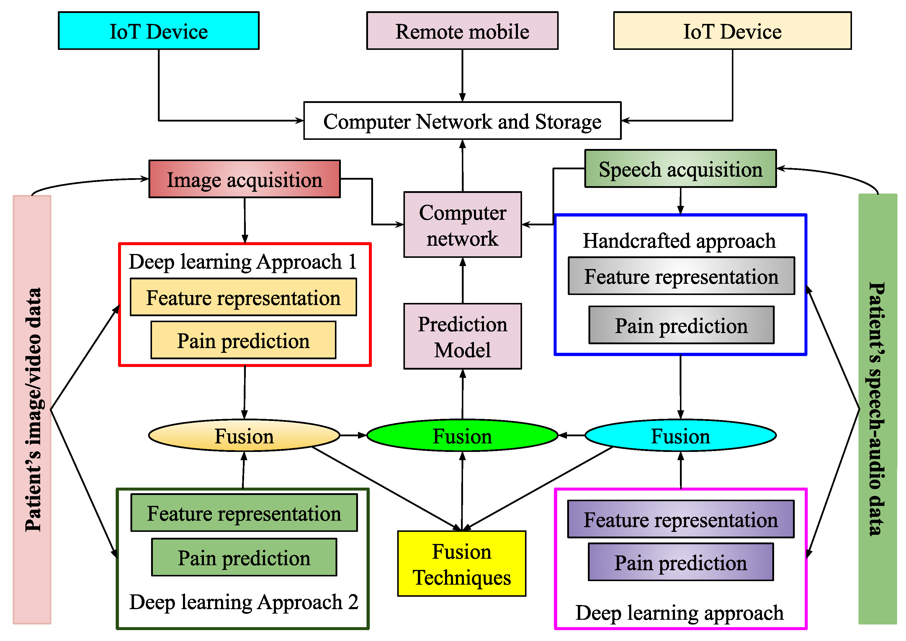
Figure 2.
The employed architecture for the proposed system.
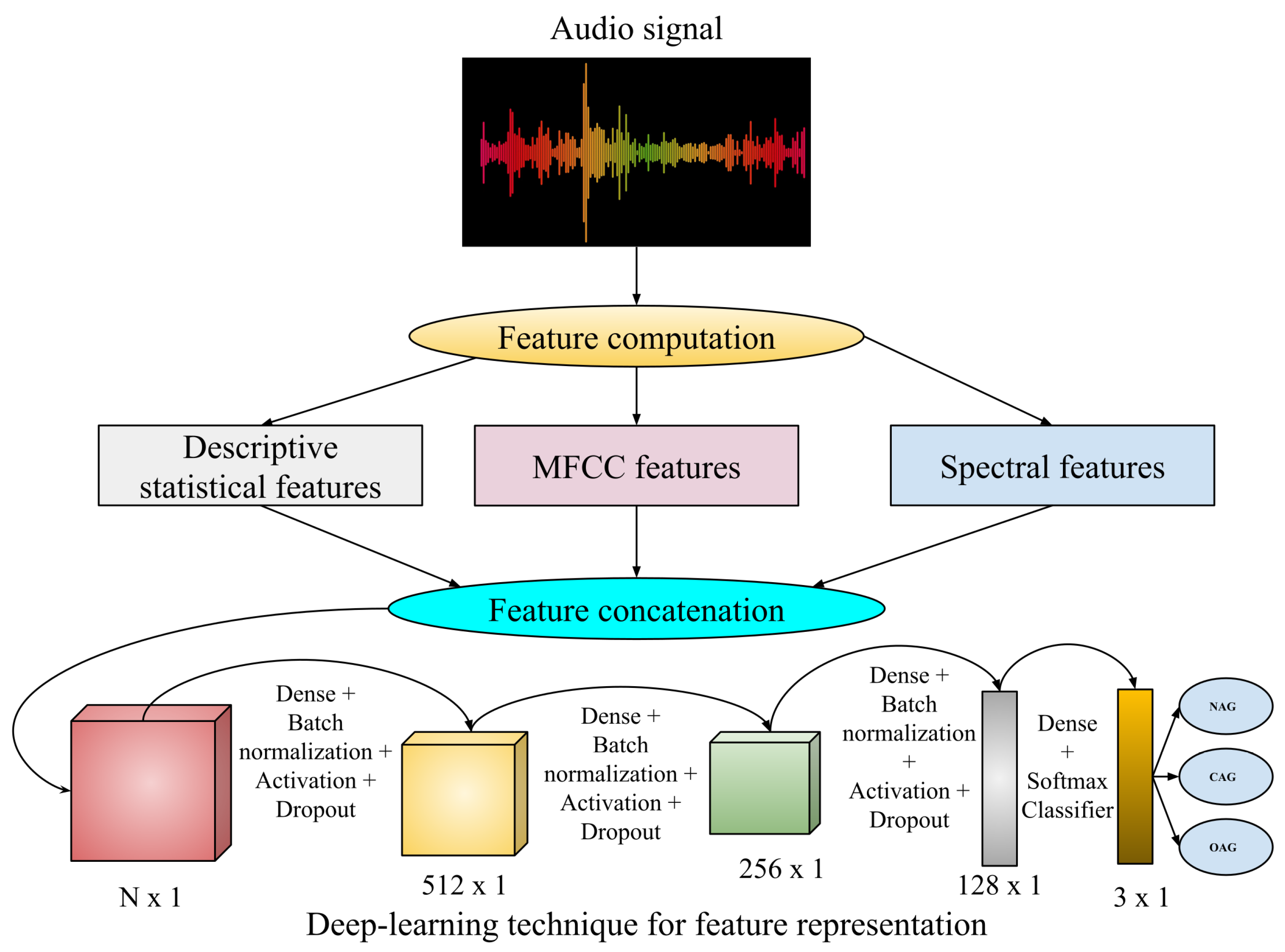
Figure 3.
The process of detecting the facial region for the input image for the proposed Image Based Pain Sentiment Analysis System.
Figure 3.
The process of detecting the facial region for the input image for the proposed Image Based Pain Sentiment Analysis System.
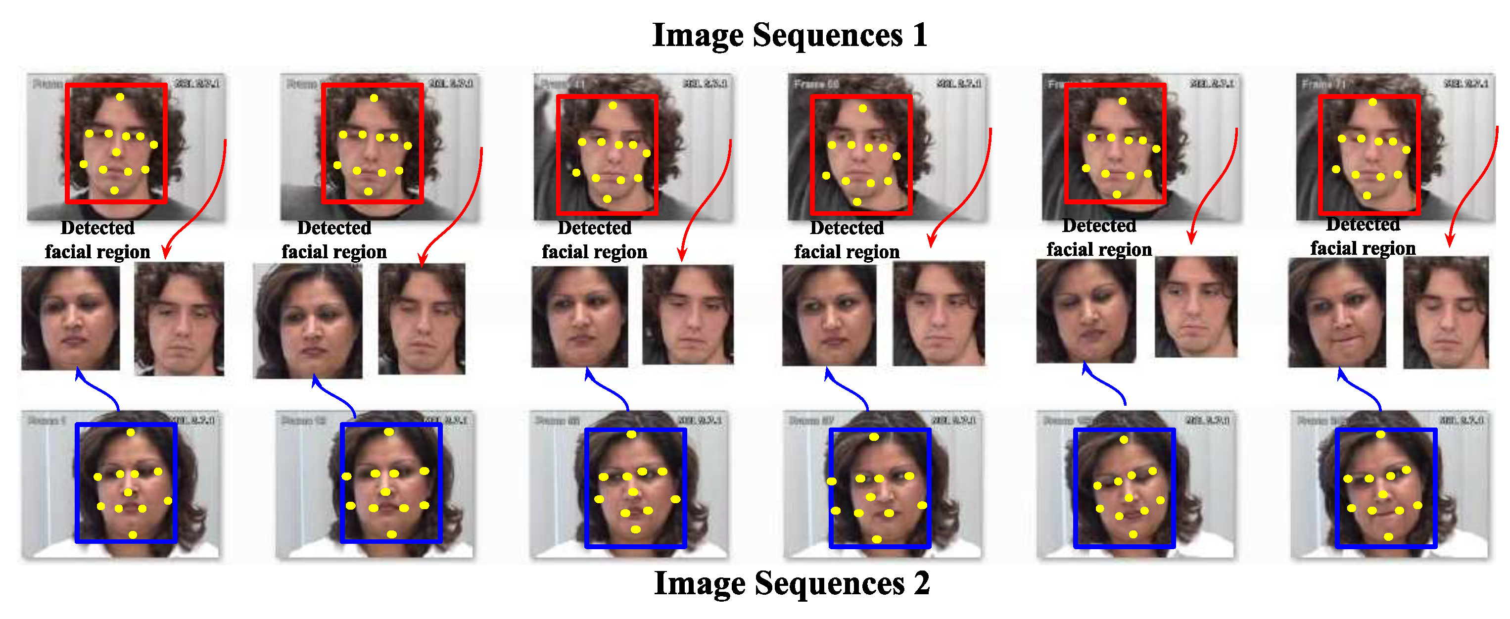
Figure 4.
Demonstration of architecture for the proposed image-based PSAS.
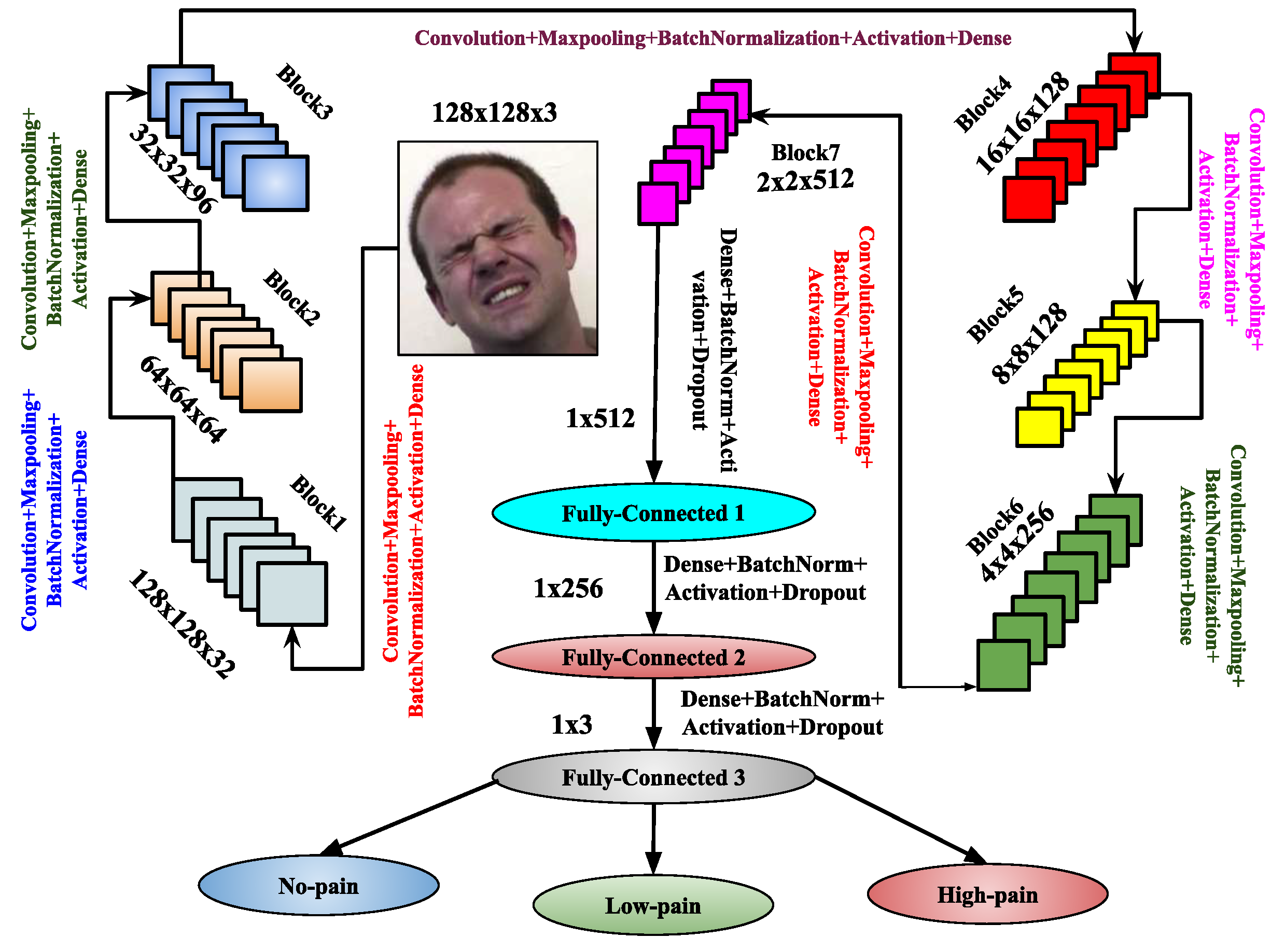
Figure 5.
Demonstration of architecture for the proposed image-based pain sentiment analysis system.
Figure 5.
Demonstration of architecture for the proposed image-based pain sentiment analysis system.
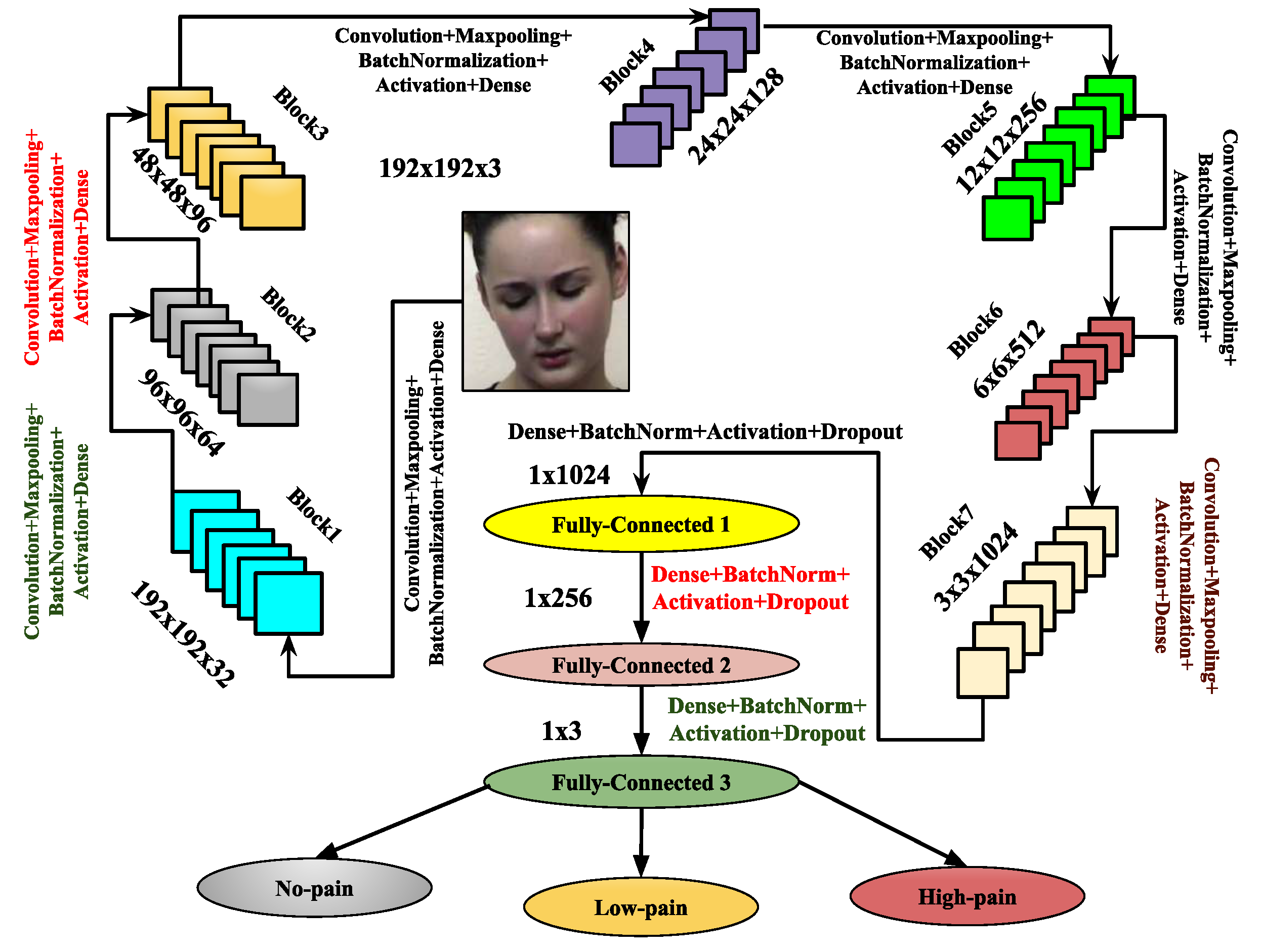
Figure 6.
Examples of some image samples from UNBC-McMaster [65] database.
Figure 6.
Examples of some image samples from UNBC-McMaster [65] database.
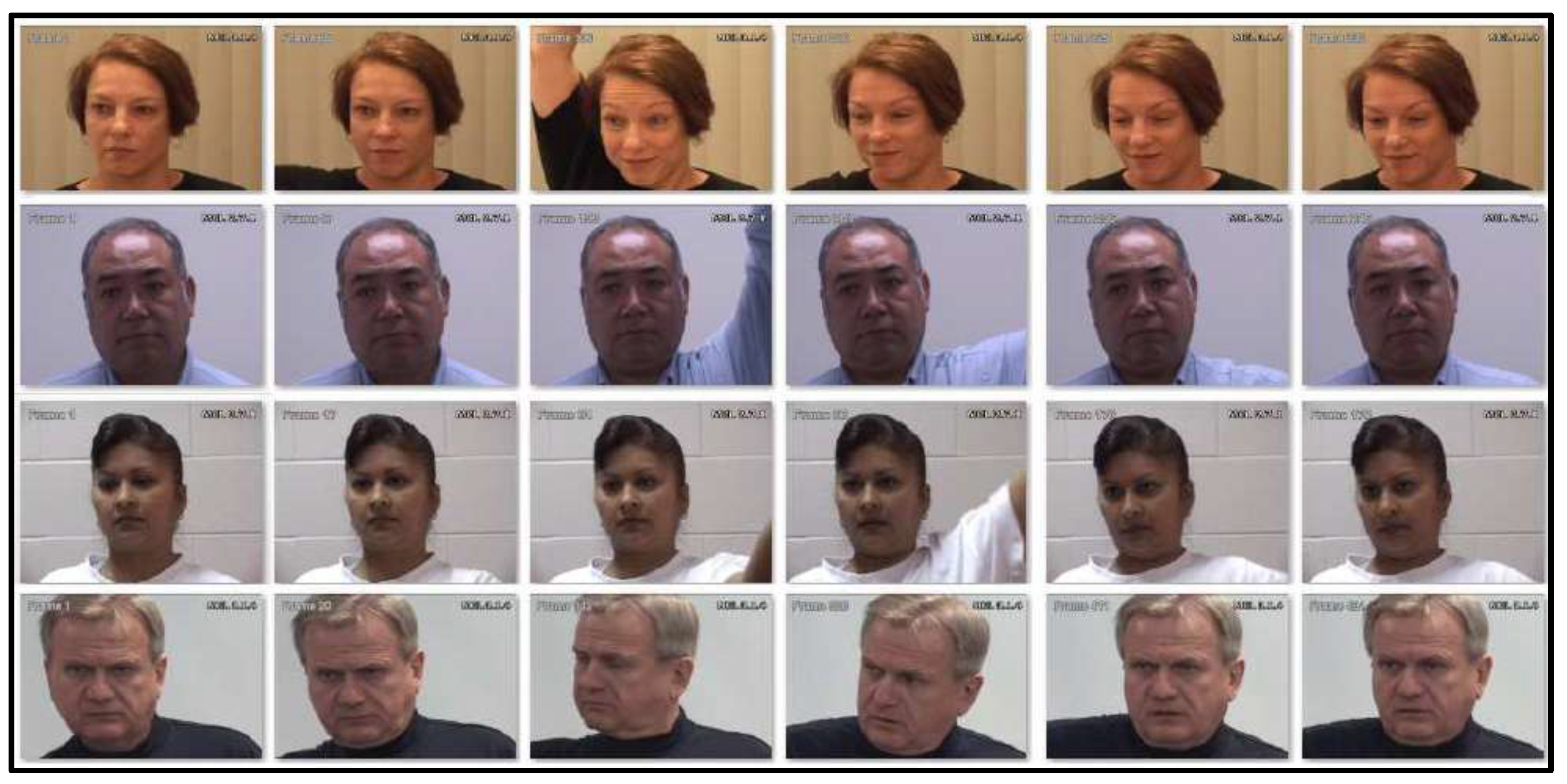
Figure 7.
Examples of some image samples from [66] database.
Figure 7.
Examples of some image samples from [66] database.
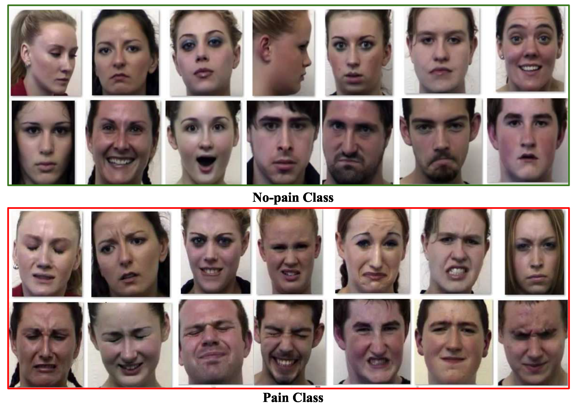
Figure 8.
Examples of some image samples from BioVid Heat Pain [67] database.
Figure 8.
Examples of some image samples from BioVid Heat Pain [67] database.
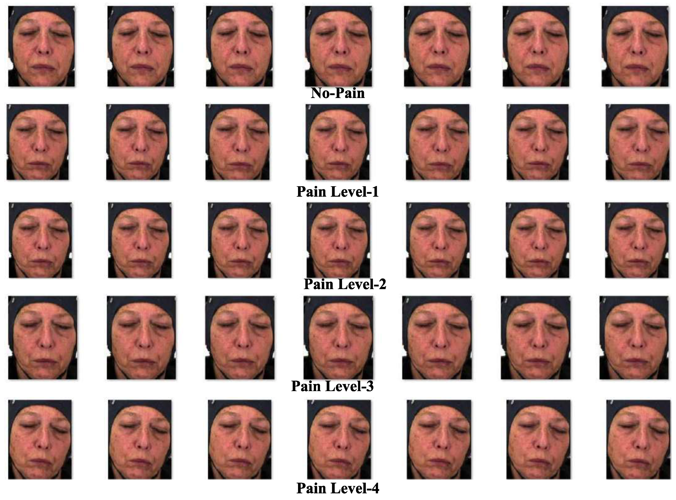
Figure 9.
Demonstration of experiments with performing the batch vs. epochs on the proposed system’s performance.
Figure 9.
Demonstration of experiments with performing the batch vs. epochs on the proposed system’s performance.
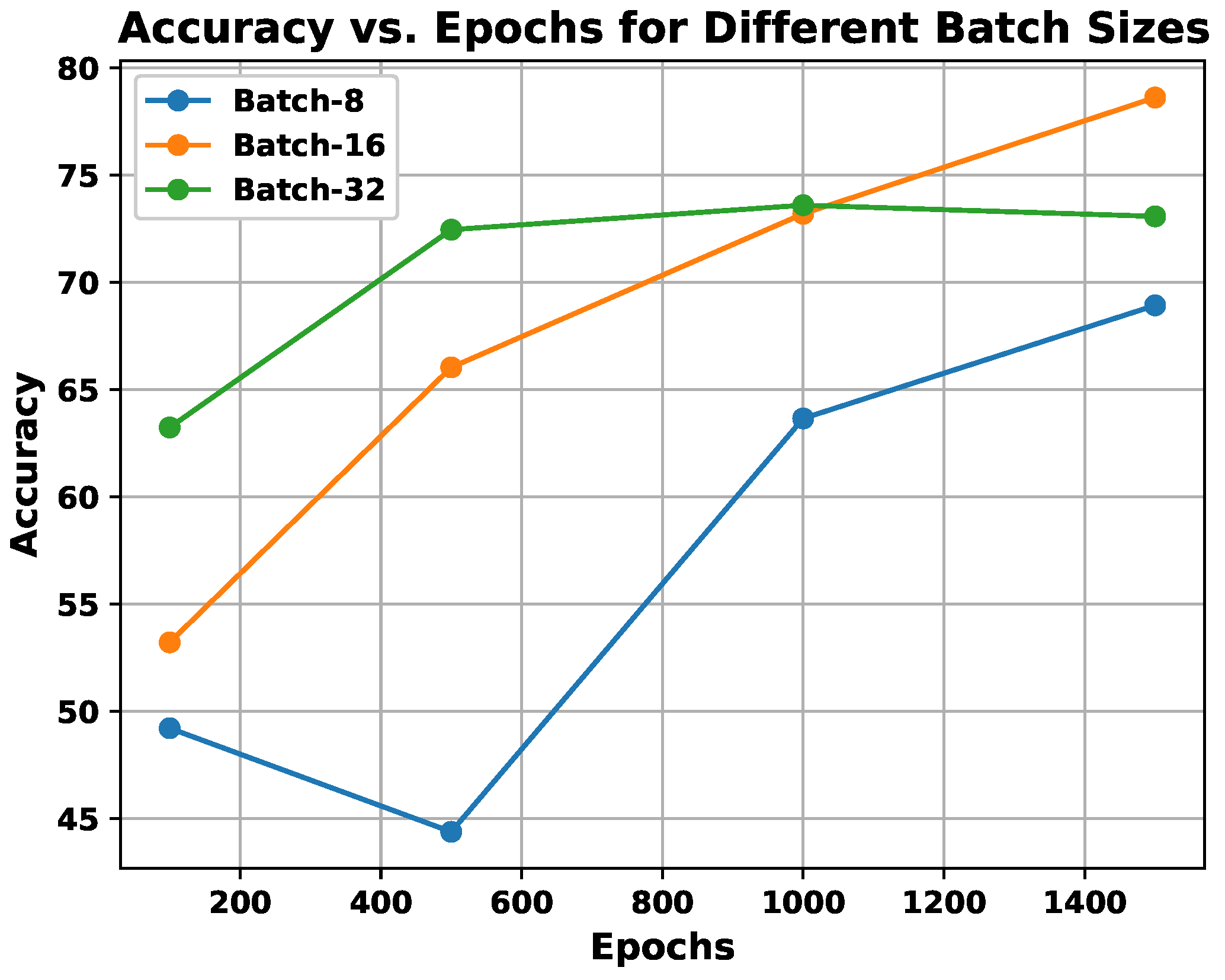
Figure 10.
Demonstration of experiments with performing the multi-resolution image analysis on the performance of the proposed system.
Figure 10.
Demonstration of experiments with performing the multi-resolution image analysis on the performance of the proposed system.
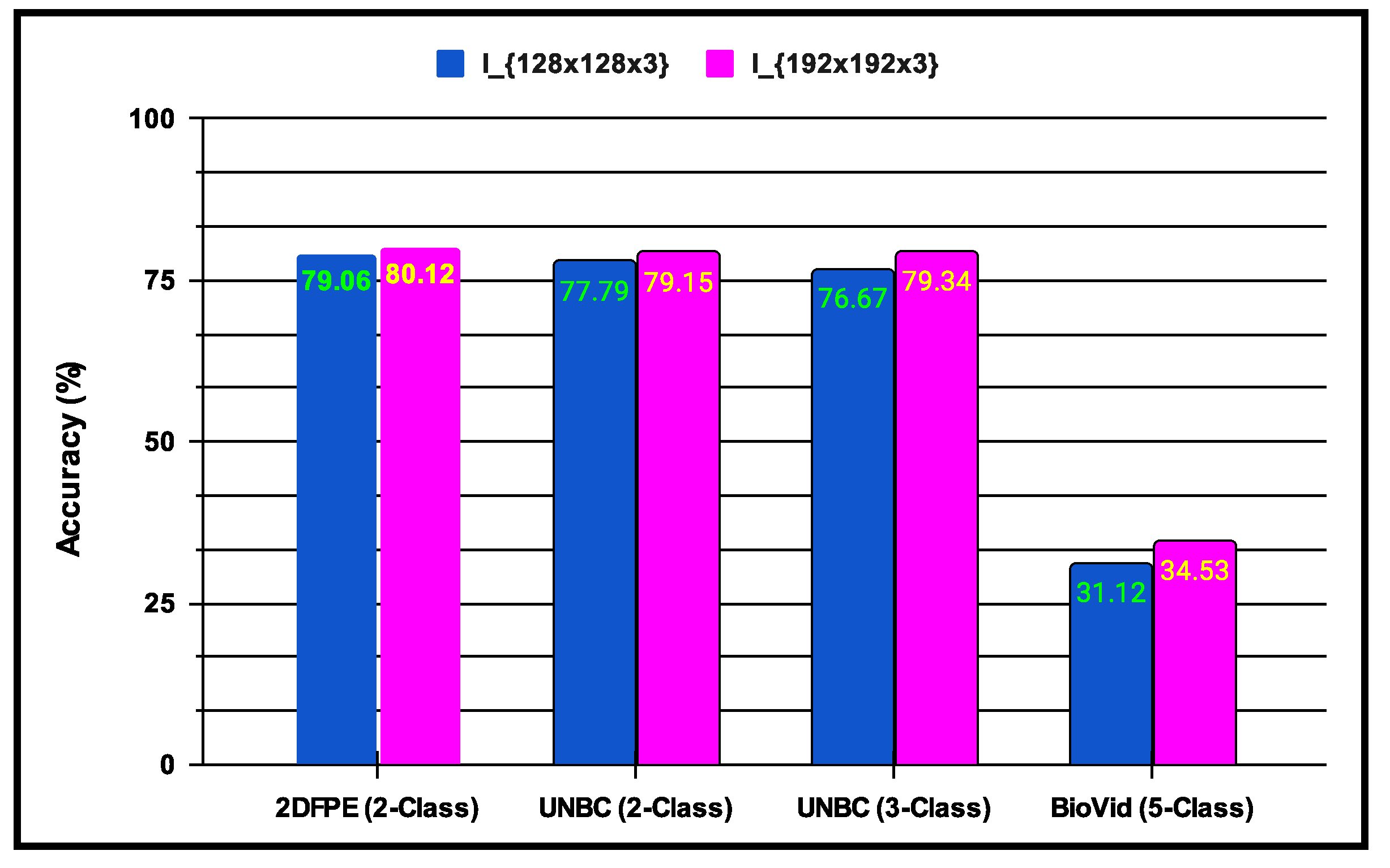
Figure 11.
Performance of the proposed pain SAS using audio features with (a) 50-50% training-testing, and (b) 75-25% training-testing sets.
Figure 11.
Performance of the proposed pain SAS using audio features with (a) 50-50% training-testing, and (b) 75-25% training-testing sets.
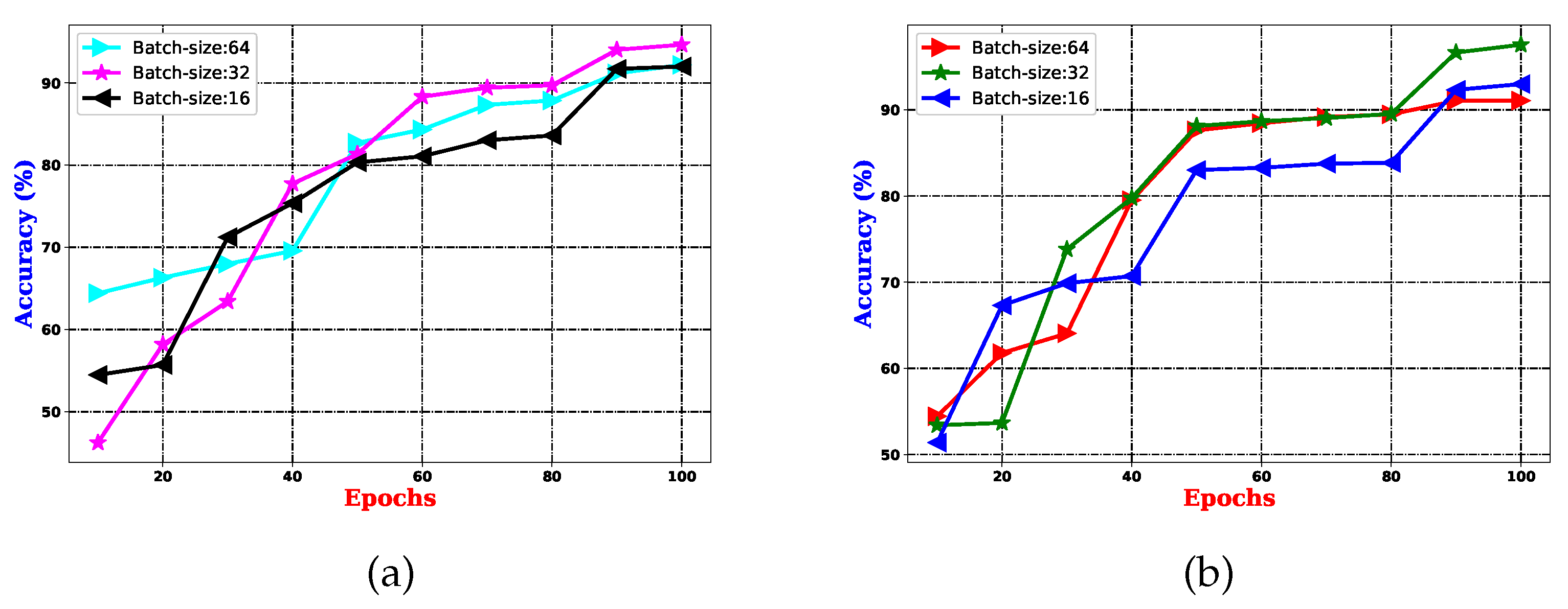
Figure 12.
Performance of the proposed pain sentiment analysis system using the performance reported in Table 9 and Figure 11.
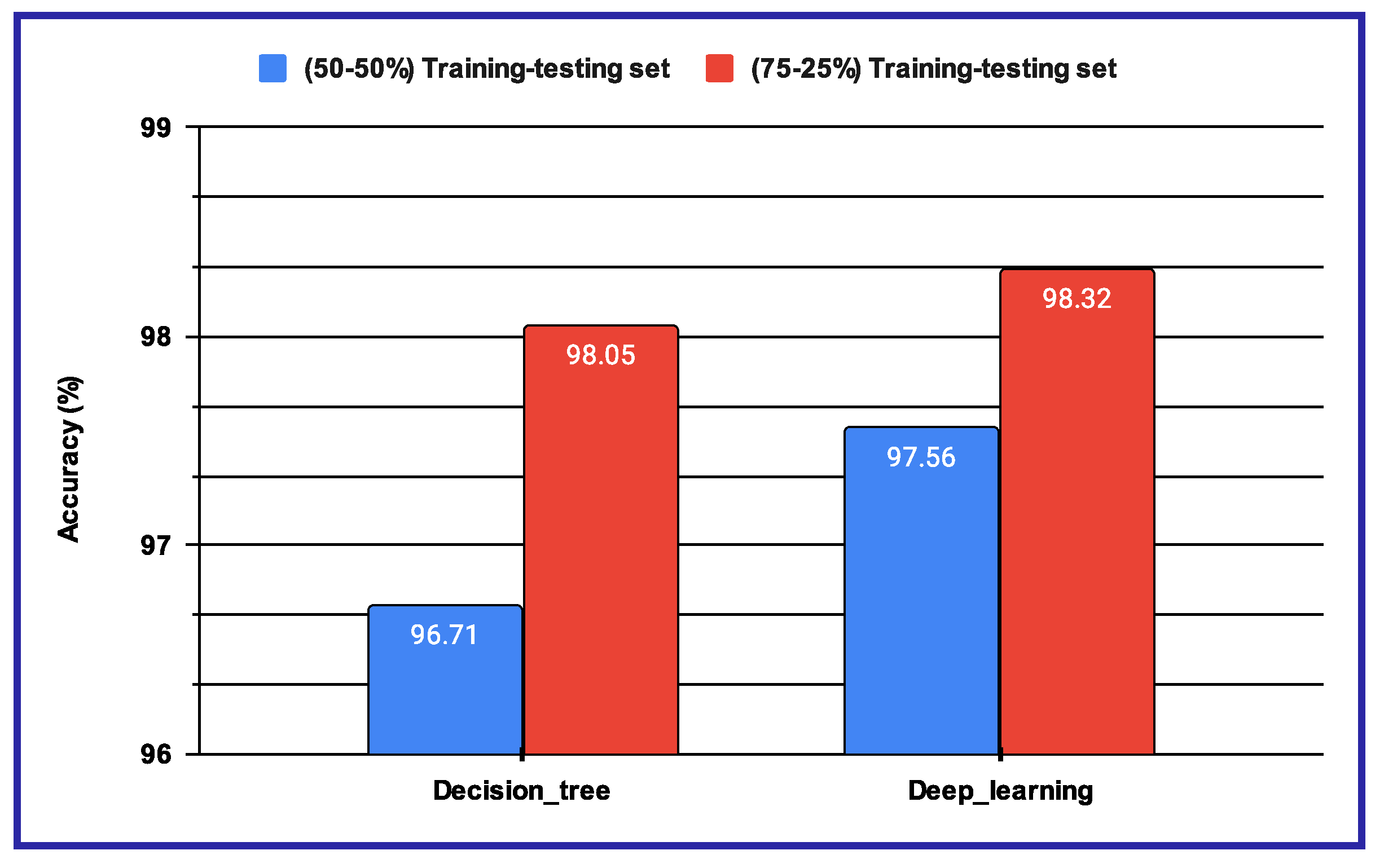
Figure 13.
Performance of the proposed (a) multimodal pain SAS () using 2-class and VIVAE databases.
Figure 13.
Performance of the proposed (a) multimodal pain SAS () using 2-class and VIVAE databases.
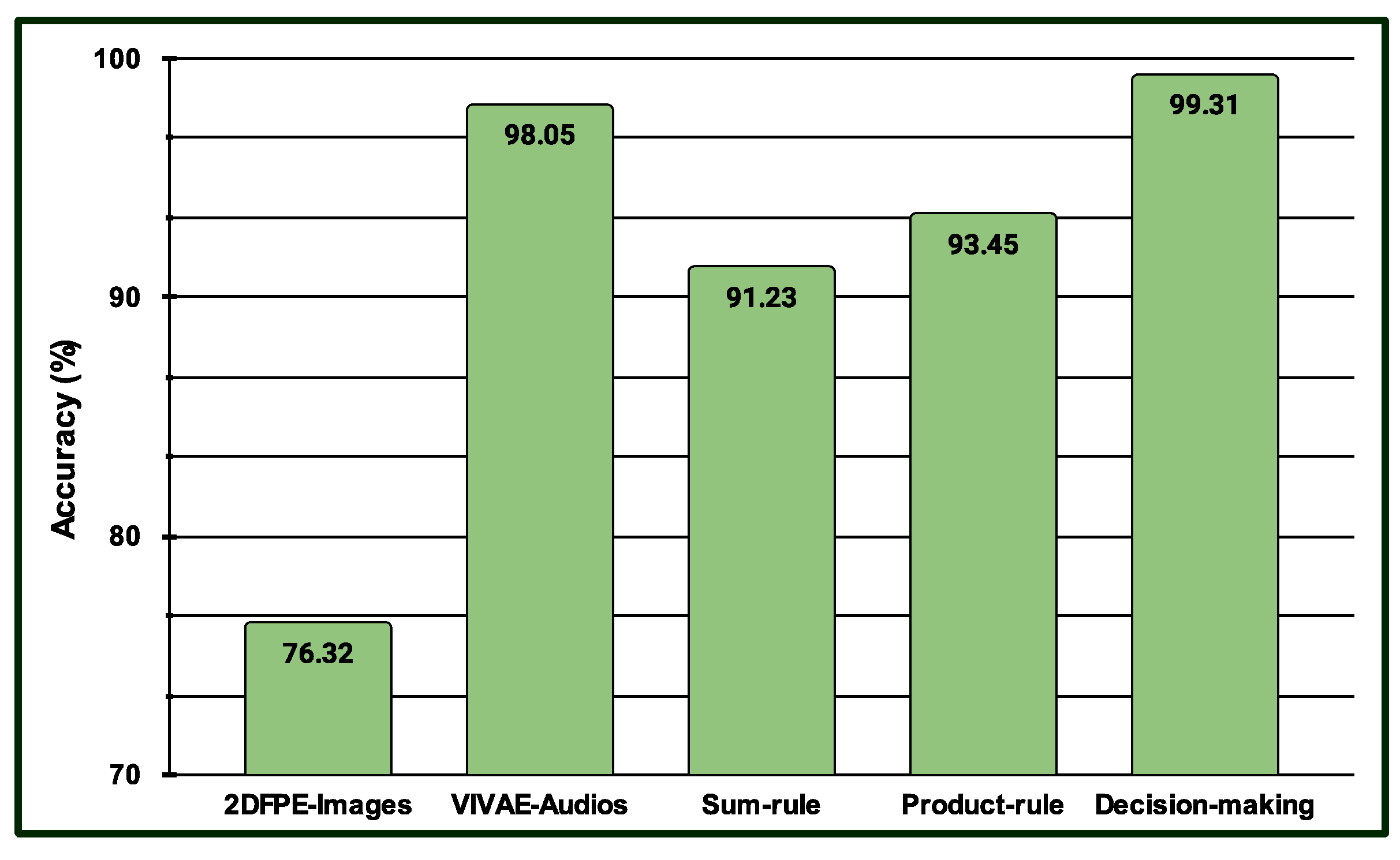
Figure 14.
Performance of the proposed multimodal pain SAS () using 3-Class UNBC-McMaster and VIVAE databases.
Figure 14.
Performance of the proposed multimodal pain SAS () using 3-Class UNBC-McMaster and VIVAE databases.
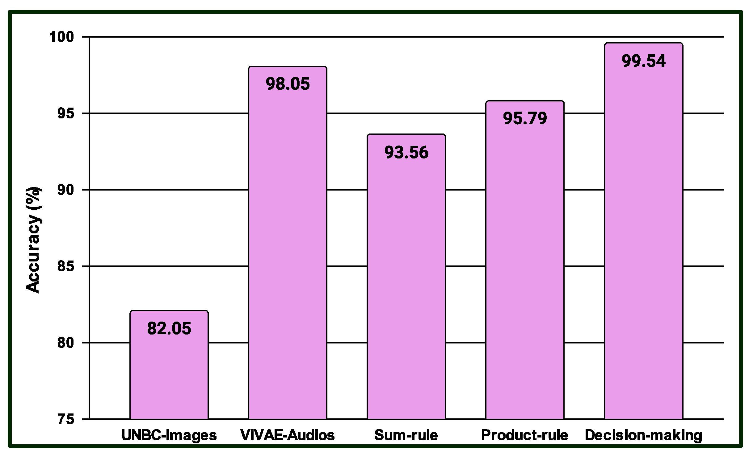
Figure 15.
Performance of the proposed multimodal pain SAS () using 4-class BioVid and VIVAE databases
Figure 15.
Performance of the proposed multimodal pain SAS () using 4-class BioVid and VIVAE databases
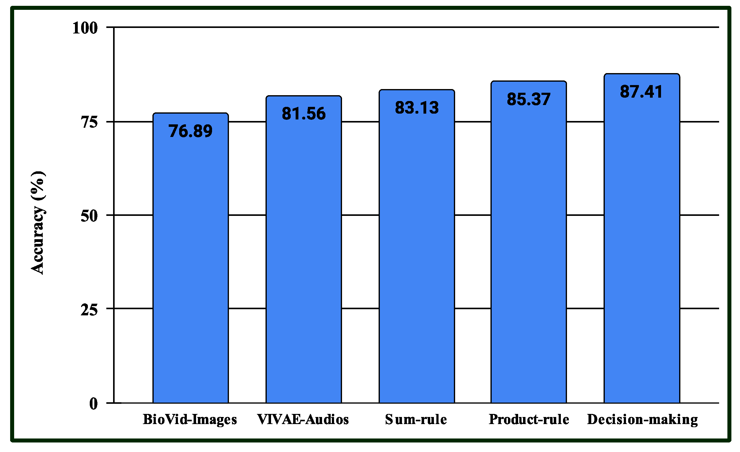

Table 1.
List of parameters required for the audio-based deep learning technique.
| Layer | Output-shape | Feature-size | Parameter |
|---|---|---|---|
| Flatten | (1, d) | (1,d) | 0 |
| Dense | (1, 512) | (1, 512) | (1 + d) x 512 |
| BatNorm | (1, 512) | (1, 512) | 2048 |
| ActRelu | (1, 512) | (1, 512) | 0 |
| Dropout | (1, 512) | (1, 512) | 0 |
| Dense | (1, 256) | (1, 256) | (1 + 512) x 256 =131328 |
| BatNorm | (1, 256) | (1, 256) | 1024 |
| ActRelu | (1, 256) | (1, 256) | 0 |
| Dropout | (1, 256) | (1, 256) | 0 |
| Dense | (1, 128) | (1,128) | (1 + 256) x 128 =32896 |
| BatNorm | (1, 128) | (1,128) | 512 |
| ActRelu | (1, 128 | (1, 128) | 0 |
| Dropout | (1, 128) | (1, 128) | 0 |
| Dense | (1, 3) | (1, 3) | (128+1) x3=387 |
| Total-Parameters | 168195 +((1+d) x512) |
||
Table 2.
The detailed description of the proposed architecture with a list of parameters required for each core building Block.
Table 2.
The detailed description of the proposed architecture with a list of parameters required for each core building Block.
| Layers | Outputshape | ImageSize | Parameters | ||||
|---|---|---|---|---|---|---|---|
| Block1 | |||||||
| Conv2D(3x3)@32 | (n,n,32) | (128, 128, 32) | 896 | ||||
| BatchNorm | (n,n,32) | (128, 128, 32) | 128 | ||||
| ActivationReLU | (n,n,32) | (128, 128, 32) | 0 | ||||
| Maxpool2D(2x2) | (n1,n1, 32), n1=n/2 | (64, 64,32) | 0 | ||||
| Dropout | (n1,n1, 32), n1=n/2 | (64, 64,32) | 0 | ||||
| Layers | Outputshape | ImageSize | Parameters | Layers | Outputshape | ImageSize | Parameters |
| Block2 | Block5 | ||||||
| Conv2D(3x3)@64 | (n1, n1, 64) | (64, 64, 64) | ((3x3x32) + 1)x64=18496 | Conv2D (3x3)@128 | (n4, n4,128) | (8, 8, 128) | ((3x3x128)+1)x128=147584 |
| BatchNorm | (n1, n1, 64) | (64, 64, 64) | 4x64 = 256 | BatchNorm | (n4, n4,128) | (8, 8, 128) | 4x128=512 |
| Activation ReLU | (n1, n1, 64) | (64 ,64 ,64) | 0 | Activation ReLU | (n4, n4,128) | (8, 8, 128) | 0 |
| Maxpool2D (2x2) | (n2, n2, 64), n2=n1/2 | (32, 32,64) | 0 | Maxpool2D (2x2) | (n5, n5,128), n5=n4/2 | (4, 4,128) | 0 |
| Dropout | (n2, n2, 64) | (32, 32,64) | 0 | Dropout | (n5, n5,128) | (4, 4,128) | 0 |
| Block3 | Block6 | ||||||
| Conv2D(3x3)@96 | (n2, n2, 96) | (32, 32, 96) | ((3x3x64)+1)x 96=55392 | Conv2D(3x3)@256 | (n5, n5, 256) | (4, 4, 256) | ((3x3x128)+1)x256=295168 |
| BatchNorm | (n2, n2, 96) | (32, 32, 96) | 4x96=384 | BatchNorm | (n5, n5, 256) | (4, 4, 256) | 4x256=1024 |
| Activation ReLU | (n2, n2, 96) | (32, 32, 96) | 0 | ActivationReLU | (n5, n5, 256) | (4, 4, 256) | 0 |
| Maxpool2D (2x2) | (n3, n3, 96), n3=n2/2 | (16, 16, 96) | 0 | Maxpool2D(2x2) | (n6, n6, 256), n6=n5/2 | (2, 2, 256) | 0 |
| Dropout | (n3, n3, 96) | (16, 16, 96) | 0 | Dropout | (n6, n6, 256) | (2, 2, 256) | 0 |
| Block4 | Block7 | ||||||
| Conv2D (3x3)@128 | (n3,n3,128) | (16,16,128) | ((3x3x96)+1)x128=110720 | Conv2D(3x3)@512 | ( n6, n6 , 512) | (2, 2, 512) | ((3x3x256)+1)x512=1180160 |
| BatchNorm | (n3,n3,128) | (16,16,128) | 4x128=512 | BatchNorm | ( n6, n6 , 512) | (2, 2, 512) | 4x512=2048 |
| Activation ReLU | (n3,n3,128) | (16,16,128) | 0 | Activation Re LU- | ( n6, n6 , 512) | (2, 2, 512) | 0 |
| Maxpool2D (2x2) | (n4,n4,128), n4=n3/2 | (8, 8, 128) | 0 | Maxpool2D(2x2) | ( n7, n7 ,512), n7=n6/2 | (1,1,512) | 0 |
| Dropout | (n4,n4,128) | (8, 8, 128) | 0 | Dropout | ( n7, n7 ,512) | (1,1,512) | 0 |
| Layer | Output Shape | Image Size | Parameter | ||||
| Flatten | (1, n7 X n7 X 512 ) | (1,512) | 0 | ||||
| Dense | (1,256) | (1,256) | (1 + 512)x 256=131328 | ||||
| Batch Normalization | (1,256) | (1,256) | 4x256=1024 | ||||
| Activation Relu | (1,256) | (1,256) | 0 | ||||
| Dropout | (1,256) | (1,256) | 0 | ||||
| Dense | (1,7) | (1,7) | (256+1)x7=1799 | ||||
| Total Parameters for The Input Image Size | 1947431 | ||||||
| Total Number of Trainable Parameters: | 1944487 | ||||||
| Non-trainable params: | 2944 | ||||||
Table 3.
The detailed description of the proposed architecture with list of parameters required for its each core building Block.
Table 3.
The detailed description of the proposed architecture with list of parameters required for its each core building Block.
| Layers | Outputshape | ImageSize | Parameters | ||||
|---|---|---|---|---|---|---|---|
| Block1 | |||||||
| Conv2D(3x3)@32 | (n,n,32) | (192, 192, 32) | 896 | ||||
| BatchNorm | (n,n,32) | (192, 192, 32) | 128 | ||||
| ActivationReLU | (n,n,32) | (192, 192, 32) | 0 | ||||
| Maxpool2D(2x2) | (n1,n1, 32), n1=n/2 | (96, 96, 32) | 0 | ||||
| Dropout | (n1,n1, 32), n1=n/2 | (96, 96, 32) | 0 | ||||
| Layers | Outputshape | ImageSize | Parameters | Layers | Outputshape | ImageSize | Parameters |
| Block2 | Block5 | ||||||
| Conv2D(3x3)@64 | (n1, n1, 64) | (96, 96, 64) | ((3x3x32) + 1)x64=18496 | Conv2D (3x3)@256 | (n4, n4, 256) | (12, 12, 256) | ((3x3x128)+1)x256=295168 |
| BatchNorm | (n1, n1, 64) | (96, 96, 64) | 4x64 = 256 | BatchNorm | (n4, n4, 256) | (12, 12, 256) | 4x256=1024 |
| Activation ReLU | (n1, n1, 64) | (96, 96, 64) | 0 | Activation ReLU | (n4, n4, 256) | (12, 12, 256) | 0 |
| Maxpool2D (2x2) | (n2, n2, 64), n2=n1/2 | (48, 48, 64) | 0 | Maxpool2D (2x2) | (n5, n5, 256), n5=n4/2 | (6, 6, 256) | 0 |
| Dropout | (n2, n2, 64) | (48, 48, 64) | 0 | Dropout | (n5, n5, 256) | (6, 6, 256) | 0 |
| Block3 | Block6 | ||||||
| Conv2D(3x3)@96 | (n2, n2, 96) | (48, 48, 96) | ((3x3x64)+1)x 96=55392 | Conv2D(3x3)@512 | (n5, n5, 512) | (6, 6, 512) | ((3x3x256)+1)x512=1180160 |
| BatchNorm | (n2, n2, 96) | (48, 48, 96) | 4x96=384 | BatchNorm | (n5, n5, 512) | (6, 6, 512) | 4x512=2048 |
| Activation ReLU | (n2, n2, 96) | (48, 48, 96) | 0 | ActivationReLU | (n5, n5, 512) | (6, 6, 512) | 0 |
| Maxpool2D (2x2) | (n3, n3, 96), n3=n2/2 | (24, 24, 96) | 0 | Maxpool2D(2x2) | (n6, n6, 512), n6=n5/2 | (3, 3, 512) | 0 |
| Dropout | (n3, n3, 96) | (24, 24, 96) | 0 | Dropout | (n6, n6, 512) | (3, 3, 512) | 0 |
| Block4 | Block7 | ||||||
| Conv2D (3x3)@128 | (n3,n3,128) | (24, 24, 128) | ((3x3x96)+1)x128=110720 | Conv2D(3x3)@1024 | (n6, n6, 1024) | (3, 3, 1024) | ((3x3x512)+1)x1024=4719616 |
| BatchNorm | (n3,n3,128) | (24, 24, 128) | 4x128=512 | BatchNorm | (n6, n6, 1024) | (3, 3, 1024) | 4x1024=4096 |
| Activation ReLU | (n3,n3,128) | (24, 24, 128) | 0 | ActivationReLU | (n6, n6, 1024) | (3, 3, 1024) | 0 |
| Maxpool2D (2x2) | (n4,n4,128), n4=n3/2 | (12, 12, 128) | 0 | Maxpool2D(2x2) | (n7, n7, 1024), n7=n6/2 | (1, 1, 1024) | 0 |
| Dropout | (n4,n4,128) | (12, 12, 128) | 0 | Dropout | (n7, n7, 1024) | (1, 1, 1024) | 0 |
| Layer | Output Shape | Image Size | Parameter | ||||
| Flatten | (1, n7 X n7 X 1024 ) | (1,1024) | 0 | ||||
| Dense | (1,256) | (1,256) | (1 + 1024)x 256=262400 | ||||
| Batch Normalization | (1,256) | (1,256) | 4x256=1024 | ||||
| Activation Relu | (1,256) | (1,256) | 0 | ||||
| Dropout | (1,256) | (1,256) | 0 | ||||
| Dense | (1,7) | (1,7) | (256+1)x7=1799 | ||||
| Total Parameters for The Input Image Size | 6654119 | ||||||
| Total Number of Trainable Parameters: | 6649383 | ||||||
| Non-trainable params: | 4736 | ||||||
Table 4.
The description of employed databases concerning image samples for 2-class, 3-class, and 5-class pain level problems.
Table 4.
The description of employed databases concerning image samples for 2-class, 3-class, and 5-class pain level problems.
| 2DFPE Database (2-class Pain levels) | |
|---|---|
| No-Pain () | 298 |
| Pain () | 298 |
| UNBC Database (2-class Pain levels) | |
| No-Pain () | 40029 |
| Pain () | 8369 |
| UNBC Database (3-class Pain levels) | |
| No-Pain (NP) () | 40029 |
| Low-Pain (LP) () | 2909 |
| High-Pain (HP) () | 5460 |
| BioVid Heat Pain Dataset (5-class Pain levels) | |
| No-Pain () | 6900 |
| Pain Level-1 () | 6900 |
| Pain Level-2 () | 6900 |
| Pain Level-3 () | 6900 |
| Pain Level-4 () | 6900 |
Table 5.
Proposed PSAS’s performance by applying Approach-1 (A1) & Approach-2 (A2) of fine-tuning and transfer learning.
Table 5.
Proposed PSAS’s performance by applying Approach-1 (A1) & Approach-2 (A2) of fine-tuning and transfer learning.
| Dataset | Using | |||
|---|---|---|---|---|
| Acc.(%) | F1-Score | Acc.(%) | F1-Score | |
| 2DFPE (2-class Pain levels) | 75.27 | 0.7563 | 72.22 | 0.7041 |
| UNBC (2-class Pain levels) | 83.11 | 0.8174 | 83.16 | 0.7918 |
| UNBC (3-class Pain levels) | 82.44 | 0.8437 | 82.36 | 0.8213 |
| BioVid (5-class Pain levels) | 34.11 | 0.3304 | 32.73 | 0.3016 |
| Dataset | Using | |||
| 2DFPE (2-class Pain levels) | 75.81 | 0.7533 | 76.14 | 0.7524 |
| UNBC (2-class Pain levels) | 84.12 | 0.7916 | 83.53 | 0.7414 |
| UNBC (3-class Pain levels) | 82.46 | 0.8334 | 82.37 | 0.8103 |
| BioVid (5-class Pain levels) | 37.45 | 0.3571 | 36.89 | 0.3518 |
Table 6.
Proposed PSAS’s performance in terms of Acc. (%) by applying fusion methods due to different CNN architectures, whereas CPL means Class Pain Levels.
Table 6.
Proposed PSAS’s performance in terms of Acc. (%) by applying fusion methods due to different CNN architectures, whereas CPL means Class Pain Levels.
| Method | 2DFPE (2-CPL) |
UNBC (2-CPL) |
UNBC (3-CPL) |
BioVid (5-CPL) |
|---|---|---|---|---|
| (A1) | 75.27 | 83.11 | 82.44 | 34.11 |
| (A2) | 72.22 | 83.16 | 82.36 | 32.73 |
| Sum-rule (A1+A2) | 75.56 | 83.47 | 82.51 | 34.67 |
| Product-rule (A1xA2) | 76.67 | 84.11 | 83.42 | 35.13 |
| Weighted Sum-rule (A1A2) | 76.37 | 84.11 | 83.15 | 35.23 |
| (A1) | 75.81 | 84.27 | 82.46 | 37.45 |
| (A2) | 76.14 | 83.53 | 82.37 | 36.89 |
| Sum-rule (A1+A2) | 76.81 | 84.69 | 82.74 | 37.89 |
| Product-rule (A1xA2) | 77.41 | 85.15 | 83.38 | 38.04 |
| Weighted Sum-rule (A1A2) | 77.23 | 85.07 | 83.17 | 37.83 |
Table 7.
Performance comparison for image-based sentiment analysis system using 2-class, 3-class, and 5-class pain sentiments problems.
Table 7.
Performance comparison for image-based sentiment analysis system using 2-class, 3-class, and 5-class pain sentiments problems.
| 3-Class UNBC-McMaster | 2-Class UNBC-McMaster | 2-Class 2DFPE | 5-Class BioVid | |||||
|---|---|---|---|---|---|---|---|---|
| Method | Acc. (%) | F1-score | Acc. (%) | F1-score | Acc. (%) | F1-score | Acc. (%) | F1-score |
| Anay et al. | 82.54 | 0.7962 | 83.71 | 0.8193 | 75.67 | 0.7391 | 27.33 | 26.89 |
| HoG | 63.19 | 0.6087 | 73.29 | 0.6967 | 68.61 | 0.6364 | 24.34 | 24.17 |
| Inception-v3 | 72.19 | 0.6934 | 76.04 | 0.7421 | 63.89 | 0.6172 | 23.84 | 22.31 |
| LBP | 65.89 | 0.6217 | 75.92 | 0.7156 | 67.34 | 0.6386 | 26.10 | 25.81 |
| Lucey et al. | 80.81 | 0.7646 | 80.73 | 0.7617 | 72.58 | 0.6439 | 29.46 | 28.63 |
| ResNet50 | 74.40 | 0.7145 | 77.79 | 0.7508 | 63.78 | 0.6154 | 28.92 | 28.78 |
| VGG16 | 74.71 | 0.7191 | 76.16 | 0.738 | 61.98 | 0.5892 | 25.64 | 23.55 |
| Werner et al. | 75.98 | 0.7233 | 76.10 | 0.7531 | 66.17 | 0.6148 | 31.76 | 29.61 |
| Proposed | 83.38 | 0.8174 | 85.07 | 0.8349 | 77.41 | 0.7528 | 37.42 | 35.84 |
Table 8.
Quantitative comparison (in Acc. (%)) of the proposed method with other competing methods for Image-based PSAS experiment with keeping , (mean performance), (standard deviation of performance), (number of tests).
Table 8.
Quantitative comparison (in Acc. (%)) of the proposed method with other competing methods for Image-based PSAS experiment with keeping , (mean performance), (standard deviation of performance), (number of tests).
| 3-Class UNBC-McMaster | ||||||
|---|---|---|---|---|---|---|
| Method | Set-1 | Set-2 | t-statistic, p-value | Remarks | ||
| Proposed (A) | 85.21 | 81.89 | 79.05 | 3.1123 | H0: Null hypothesis; H1: Alternative hypothesis | |
| Anay et al. (B) | 83.12 | 80.45 | 84.51 | 0.18 | 0.1942, | H0 is accepted, |
| HoG (C) | 69.74 | 64.56 | 65.21 | 0.25 | 10.31, | H0 is rejected, |
| Inception-v3 (D) | 74.31 | 72.61 | 71.39 | 2.42 | 7.54, | H0 is rejected, |
| LBP (E) | 71.36 | 62.72 | 67.04 | 37.32 | 3.5674, | H0 is rejected, |
| Lucey et al. (F) | 82.78 | 80.45 | 80.21 | 12.33 | 7.54, | H0 is rejected, |
| ResNet50 (G) | 76.72 | 75.91 | 76.32 | 0.33 | 4.23, | H0 is rejected, |
| VGG16 (H) | 73.33 | 76.23 | 74.78 | 4.21 | 3.97, | H0 is rejected, |
| Werner et al. (I) | 75.89 | 74.52 | 75.20 | 0.94 | 4.64, | H0 is rejected, |
| 2-Class UNBC-McMaster | ||||||
| Method | Set-1 | Set-2 | t-statistic, p-value | Remarks | ||
| Proposed (A) | 87.43 | 85.81 | 79.05 | 3.1123 | H0: Null hypothesis; H1: Alternative hypothesis | |
| Anay et al. (B) | 82.17 | 84.29 | 84.21 | 2.14 | 4.4314, | H0 is rejected, |
| HoG (C) | 76.33 | 75.01 | 74.96 | 0.25 | 10.31, | H0 is rejected, |
| Inception-v3 (D) | 77.45 | 75.19 | 76.32 | 2.55 | 7.40, | H0 is rejected, |
| LBP (E) | 73.23 | 76.93 | 73.81 | 3.70 | 7.39, | H0 is rejected, |
| Lucey et al. (F) | 82.19 | 81.89 | 82.04 | 0.04 | 5.55, | H0 is rejected, |
| ResNet50 (G) | 79.31 | 78.05 | 78.68 | 0.79 | 7.73, | H0 is rejected, |
| VGG16 (H) | 77.45 | 71.38 | 74.41 | 18.42 | 3.88, | H0 is rejected, |
| Werner et al. (I) | 74.38 | 73.67 | 74.03 | 0.25 | 14.24, | H0 is rejected, |
| 2-Class 2DFPE | ||||||
| Method | Set-1 | Set-2 | t-statistic, p-value | Remarks | ||
| Proposed (A) | 77.41 | 81.91 | 79.66 | 10.12 | H0: Null hypothesis; H1: Alternative hypothesis | |
| Anay et al. (B) | 75.67 | 76.06 | 75.87 | 0.08 | 1.68, | H0 is accepted, |
| HoG (C) | 68.61 | 72.71 | 70.66 | 8.40 | 2.95, | H0 is rejected, |
| Inception-v3 (D) | 63.89 | 65.07 | 64.48 | 0.70 | 6.52, | H0 is rejected, |
| LBP (E) | 67.34 | 69.47 | 68.40 | 2.27 | 4.52, | H0 is rejected, |
| Lucey et al. (F) | 72.58 | 75.01 | 73.80 | 2.95 | 2.29, | H0 is accepted, |
| ResNet50 (G) | 63.78 | 65.39 | 64.59 | 1.30 | 6.30, | H0 is rejected, |
| VGG16 (H) | 61.98 | 64.14 | 63.06 | 2.33 | 6.65, | H0 is rejected, |
| Werner et al. (I) | 69.05 | 71.37 | 70.21 | 2.69 | 3.73, | H0 is rejected, |
| 5-Class BioVid | ||||||
| Method | Set-1 | Set-2 | t-statistic, p-value | Remarks | ||
| Proposed (A) | 37.67 | 37.81 | 37.42 | 0.62 | H0: Null hypothesis; H1: Alternative hypothesis | |
| Anay et al. (B) | 28.15 | 26.41 | 26.96 | 2.13 | 15.4437, | H0 is rejected, |
| HoG (C) | 23.05 | 25.24 | 24.34 | 2.62 | 17.7968, | H0 is rejected, |
| Inception-v3 (D) | 22.78 | 24.89 | 23.84 | 2.23 | 13.15, | H0 is rejected, |
| LBP (E) | 25.89 | 26.31 | 26.10 | 0.09 | 52.58, | H0 is rejected, |
| Lucey et al. (F) | 29.78 | 29.15 | 29.46 | 0.20 | 25.64, | H0 is rejected, |
| ResNet50 (G) | 28.56 | 29.28 | 28.92 | 0.26 | 24.049, | H0 is rejected, |
| VGG16 (H) | 25.09 | 26.18 | 25.64 | 0.59 | 22.03, | H0 is rejected, |
| Werner et al. (I) | 31.34 | 32.17 | 31.76 | 0.34 | 14.22, | H0 is rejected, |
Table 9.
Performance of the proposed audio-based pain sentiment analysis system corresponding to machine learning classifiers
Table 9.
Performance of the proposed audio-based pain sentiment analysis system corresponding to machine learning classifiers
| 50-50% training-testing set | 75-25% training-testing set | |||||||
|---|---|---|---|---|---|---|---|---|
| Statistical features | ||||||||
| Classifier | Accuracy | Precision | Recall | F1-Score | Accuracy | Precision | Recall | F1-Score |
| Logistic-Regression | 49.56 | 24.76 | 49.56 | 33.52 | 50.21 | 25.12 | 50.21 | 33.43 |
| K-Nearest-Neighbors | 75.11 | 58.17 | 75.11 | 64.47 | 52.41 | 50.43 | 50.63 | 49.22 |
| Decision-Tree | 75.11 | 58.17 | 75.11 | 64.47 | 50.21 | 25.12 | 50.21 | 33.43 |
| Support-Vector-Machine | 49.56 | 24.76 | 49.56 | 33.52 | 50.21 | 25.14 | 50.21 | 33.43 |
| MFCC features | ||||||||
| Logistic-Regression | 52.23 | 35.63 | 52.23 | 39.52 | 75.34 | 58.18 | 75.07 | 64.74 |
| K-Nearest-Neighbors | 52.23 | 35.63 | 52.23 | 39.52 | 75.66 | 63.29 | 75.22 | 67.39 |
| Decision-Tree | 95.18 | 93.52 | 92.38 | 92.73 | 97.57 | 96.45 | 95.81 | 95.08 |
| Support-Vector-Machine | 26.27 | 9.63 | 26.41 | 13.48 | 97.43 | 96.21 | 95.72 | 94.69 |
| Spectra features | ||||||||
| Logistic-Regression | 49.71 | 33.12 | 49.76 | 39.44 | 75.18 | 58.37 | 75.18 | 64.77 |
| K-Nearest-Neighbors | 75.13 | 58.17 | 75.21 | 64.53 | 75.18 | 53.37 | 75.18 | 64.77 |
| Decision-Tree | 96.45 | 95.41 | 95.43 | 94.21 | 98.51 | 97.49 | 97.43 | 97.19 |
| Support-Vector-Machine | 96.31 | 95.23 | 94.24 | 93.19 | 75.18 | 58.37 | 75.18 | 64.77 |
Table 10.
Computational complexity in sec. for the proposed pain detection systems.
| Data Type | Image Classification | Audio Classification | |
|---|---|---|---|
| CNN Models | |||
| Trainable Parameters | 1947431 | 6654119 | 281,603 |
| Non-Trainable Parameters | 2944 | 4736 | 1,792 |
| Total Parameters | 1944487 | 6649383 | 283,395 |
| Time | 1.04 | 1.06 | 0.43 |
Disclaimer/Publisher’s Note: The statements, opinions and data contained in all publications are solely those of the individual author(s) and contributor(s) and not of MDPI and/or the editor(s). MDPI and/or the editor(s) disclaim responsibility for any injury to people or property resulting from any ideas, methods, instructions or products referred to in the content. |
© 2024 by the authors. Licensee MDPI, Basel, Switzerland. This article is an open access article distributed under the terms and conditions of the Creative Commons Attribution (CC BY) license (http://creativecommons.org/licenses/by/4.0/).
Copyright: This open access article is published under a Creative Commons CC BY 4.0 license, which permit the free download, distribution, and reuse, provided that the author and preprint are cited in any reuse.


