
Submitted:
08 December 2024
Posted:
09 December 2024
You are already at the latest version
Abstract
Sharp, asymptotic estimates of classical and generalized rising/falling Pochhammer's products having positive arguments are presented on the basis of Stirling's approximation formula for $\Gamma$ function.
Keywords:
approximation
; error term
; estimate
; Gamma function
; inequality
; Pochhammer's product
; shifted factorial
MSC: 26D20, 41A60, 65B99 (11Y99)
1. Introduction
Pochhamer’s products or shifted factorials, falling (lower) and rising (upper), are often encountered in pure and applied mathematics and in several exact sciences too. For example, we meet them in combinatorics, number theory, probability, statistics, statistical physics, etc. These products are closely related to the famous function which is well accessible also in a numerical sense.
The classical rising Pochhammer’s product1 of the order and the basis ,
can be expressed, for , in terms of function as
There are only a few articles on approximating the Pochhammer product. One of them is [3], where are given several approximations to the products in question. In our paper, we would like to present sharper and more general results than those given in [3].
The last equation above suggests the most useful extension of the classical rising discrete-order Pochhammer’s factorial to a continuous-order Pochhammer’s factorial by setting the following definition.
Definition 1.
The rising Pochhammer’s factorial is defined as
Obviously, and , for .
Lemma 1.
For , we have
Proof.
Considering Definition 1, we have, for ,
□
The classical falling Pochhammer’s product of order and basis ,
can be expressed by the rising Pochhammer’s factorial as
for an integer n and a real x satisfying . Therefore, we extend the domain of the falling Pochhammer’s factorial to continuous case setting
Moreover, since , for , we set the next definition.
Definition 2.
The falling Pochhammer’s factorial we define as
Obviously, and , for .
2. Auxiliary Result (Approximation of Function)
The Stirling approximation formula of order for function says that for we have [2] [sect. 9.5]
where
and, for some ,
The numbers , , , …are known as the Bernoulli coefficients2. We have, for example,
with the estimates , , , , , , .
As a consequence, we have for the (continuous) factorial function the expression (the Stirling factorial formula)
3. Approximations to Pochhammer’s Products
According to (7) we have, for ,
At small x the estimate (11) becomes useless. Therefore, in (10) we replace x with , where m is a positive integer, not being too large. Using the Formulas (10) and (11) together with (2), we find an asymptotic approximation of the generalized Pochhammer’s rising product given in the next theorem.
Theorem 1.
Example 1.
For we have
and
with .
For and any integer we obviously have . Moreover, setting and in Theorem 1, we get a more accurate estimate, given in the next corollary4.
Corollary 1.
For , there hold the following inequalities:
Figure 1 illustrates5 the relations (17) and (18) by plotting the graphs of the functions and , together with the graph (continuous line) of the function , which nearly coincides with the function .
Remark 1.
Corollary 2.
For and for integers , satisfying , the approximation , given in Theorem 1, has the relative error
estimated as
Proof.
According to Theorem 1, using Taylor’s formula, we obtain, for some ,
Now, for integers , satisfying , and for , we have . Consequently, referring to (16) and (23), we estimate . Hence, considering (25), we get
□
The immediate consequence of Corollary 2 is the next corollary.
Corollary 3.
For and for integers , satisfying , the inequalities
hold.
Example 2.
Setting and in Corollary 3 we obtain the following double inequalities:
true for and , and
valid for and .
The inequalities in (28) are illustrated in Figure 2, where the dashed line represents the graph of the function and the continuous line, compressed between the nearly coinciding graphs of the functions , represents the graph of the function .
We are interested in how the sequence varies. Indeed, thanks to Theorem 1, for and integers , we have
Therefore, for integers and , for real , and for the difference ,
using (16), we estimate
The inequalities (31) can be used to estimate the error by using the appropriate , which specifies a negligibly small (see (22)) and thus provides a useful estimate for . Figure 3 and Figure 4 illustrate the estimate (31), for , by showing the graphs of the functions7 and , cramming the graphs of the functions .
Remark 2
For , the quantity is called p–factorial. The discrete factorial function is extended continuously, for real , as . Immediately from Theorem 1 we read the next corollary, which presents a formula for that does not contain the constant .
Corollary 4
(approximation of continuous factorial function). For and integers we have8
for some from the interval .
Using Definition 2 and Theorem 1 we obtain the approximation of generalized Pochhammer’s falling product presented in the next theorem.
Theorem 2.
For real , satisfying and for integers , we have the equality
where , that is
with defined in (15), and
Remark 3.
Using Definition 2 and Corollary 3 we read the next result.
Corollary 5.
For real satisfying and for integers such that , the inequalities
and
hold.
Thanks to Corollary 5, the approximation has the relative error estimated as
true for that meet all conditions given in Corollary 5.
4. Sequences of Classical Binomial Coefficients
According to (3), the binomial coefficient “x over n”,
can be expressed using the upper Pochhammer product in the way, given in the next Proposition.
Proposition 1.
For every real x and any integer , we have10
Proof.
The first and the last cases are obvious. Relating to the second one, for , we have11
□
Thanks to Proposition 1, Theorem 1 and (9), we present the following three examples.
Example 3.
Using and in Theorem 1 and in (9), we obtain, for some and ,
Thus, for every and some and , we have
Hence,
Figure 7 shows the graphs of the sequences and , left and right respectively.
Example 4.
Setting and in Theorem 1 and in (9), we get, for some and ,
Therefore, for any , using some and , we find
Hence,
Figure 8 shows the graphs of the sequences and , left and right respectively.
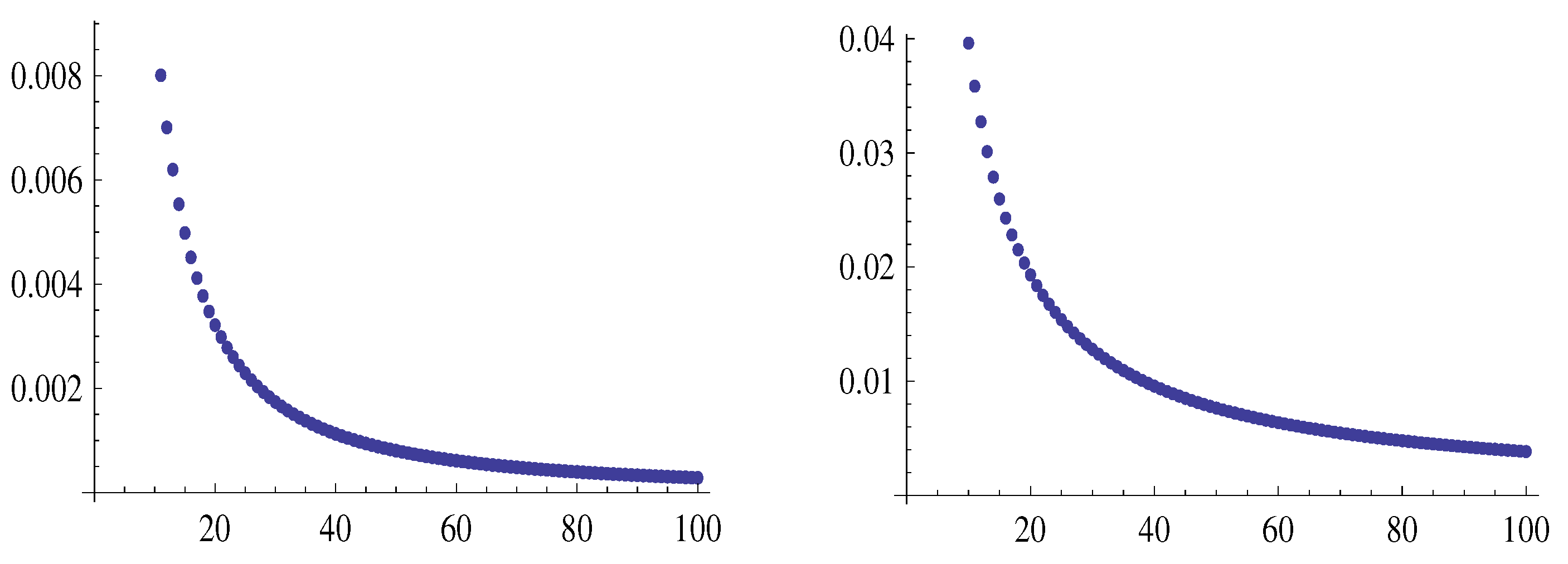
Example 5.
Figure 9 shows the graphs of the sequences and , left and right respectively.
Remark 4.
More about binomial coefficients can be find in [4].
References
- M. Abramowitz and I. A. Stegun Handbook of Mathematical Functions, 9th edn, Dover Publications, New York, 1974.
- R.L. Graham, D.E. Knuth and O. Patashnik, Concrete Mathematics, Addison-Wesley, Reading, MA, 1994.
- Lampret, V. Approximating real Pochhammer products: a comparison with powers. Cent. Eur. J. Math. 2009, 7, 493–505. [Google Scholar] [CrossRef]
- Lampret, V. Accurate approximations of classical and generalized binomial coefficients. Comput. Appl. Math. 2024, 43, 341. [Google Scholar] [CrossRef]
- Robbins, H. A Remark on Stirling Formula. Amer. Math. Monthly 1995, 62, 26–29. [Google Scholar]
- S. Wolfram, Mathematica, version 7.0, Wolfram Research, Inc., 1988–2009.
| 1 | Leo August Pochhammer, 1841–1920 |
| 2 | The positive numbers are called the Bernoulli numbers. |
| 3 | considering , by definition |
| 4 | which can be improved by increasing m
|
| 5 | All figures in this paper are produced using Mathematica [6]. |
| 6 | considering the estimate , for
|
| 7 | with
|
| 8 | taking into account the definition . |
| 9 | interesting for a larger m
|
| 10 | For , the floor symbol means the integer part of x. |
| 11 | considering the equality , for , true by definition |
| 12 | using the identity
|
Figure 1.
The graphs of the functions , and from Corollary 1.
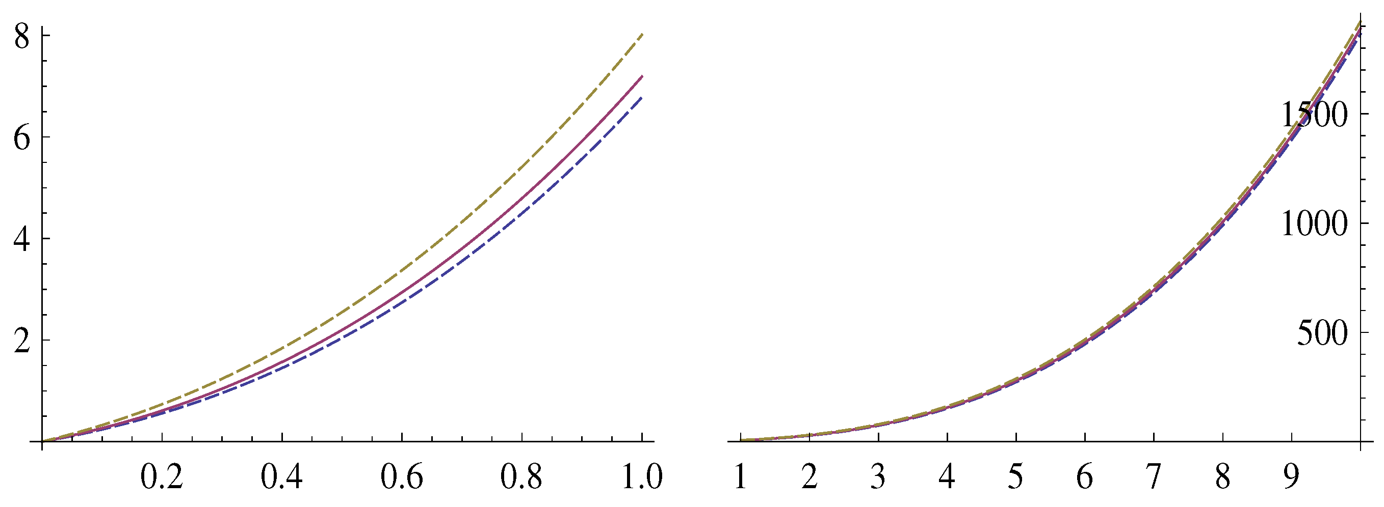
Figure 2.
The graph of the function (dashed line) and the practically coinciding graphs of the functions (continuous line).
Figure 2.
The graph of the function (dashed line) and the practically coinciding graphs of the functions (continuous line).

Figure 3.
The graphs of the functions .
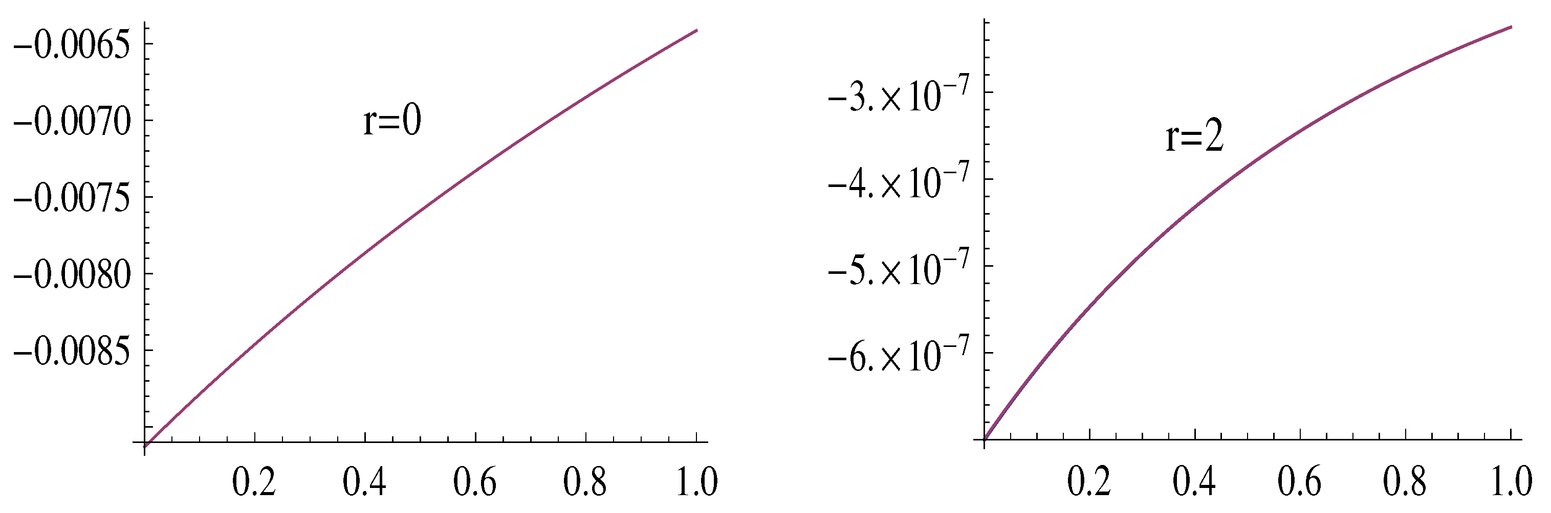
Figure 4.
The graphs of the functions .
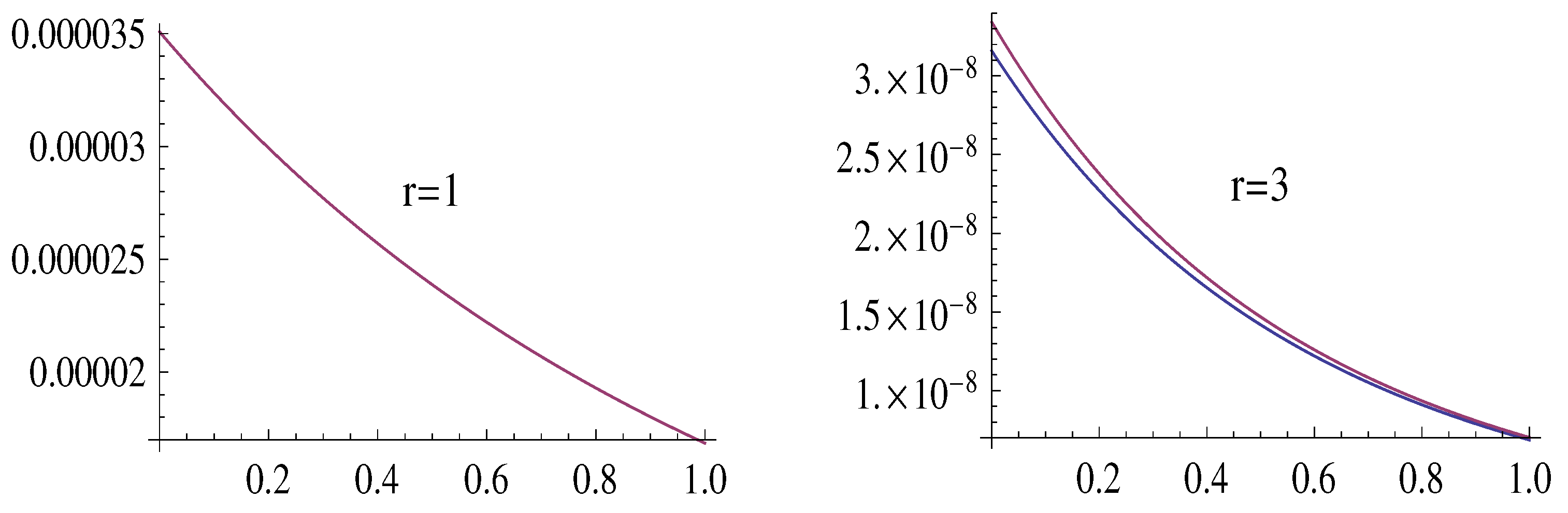
Figure 5.
The graphs of the functions .

Figure 6.
The graphs of the functions .
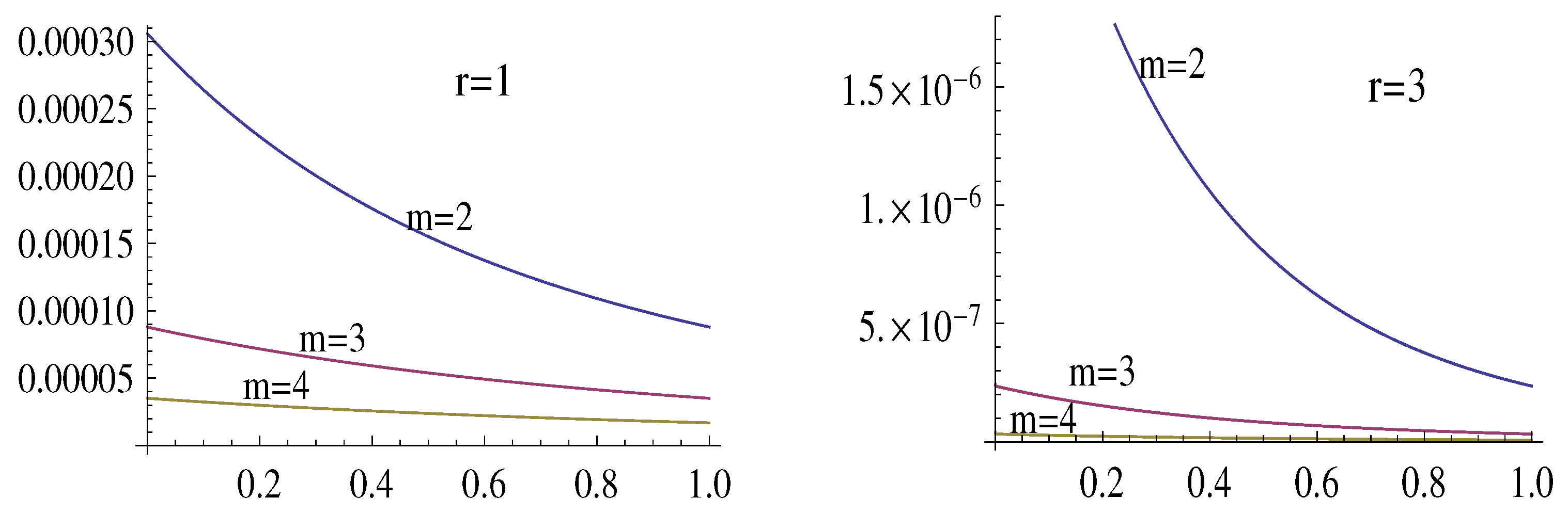
Figure 7.
The graphs of the sequences and , left and right respectively.
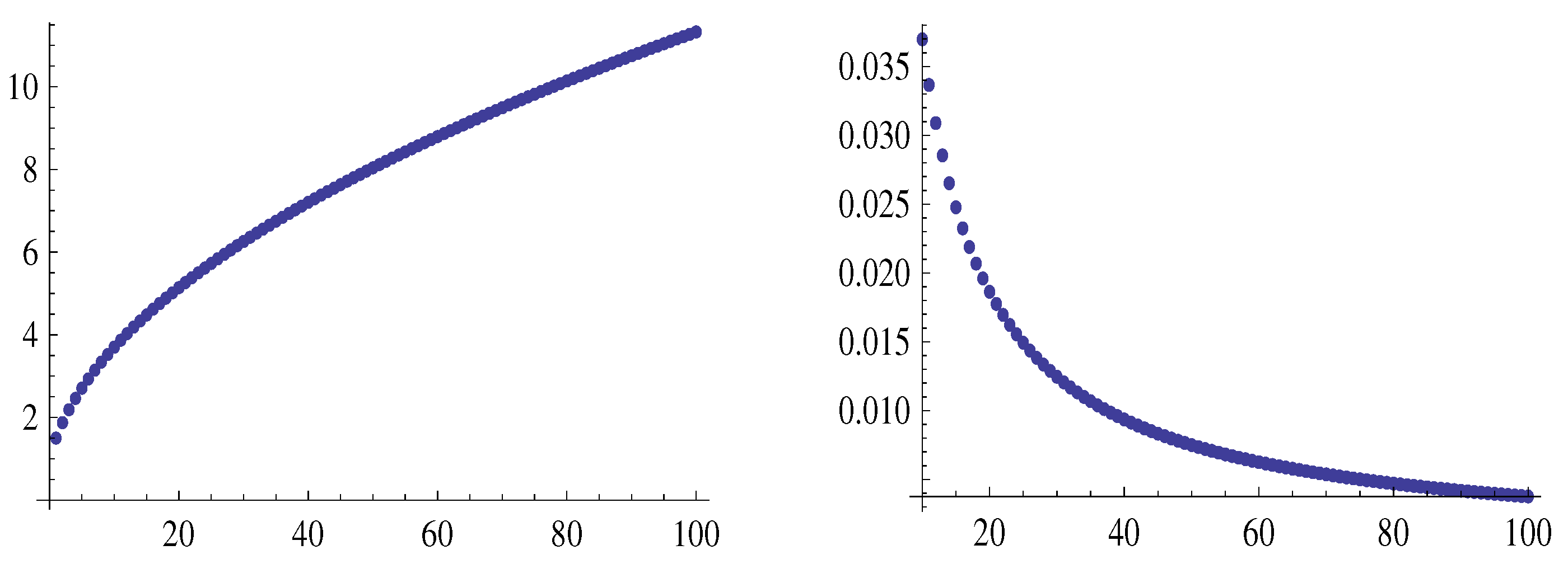
Figure 8.
The graphs of the sequences and , left and right respectively.
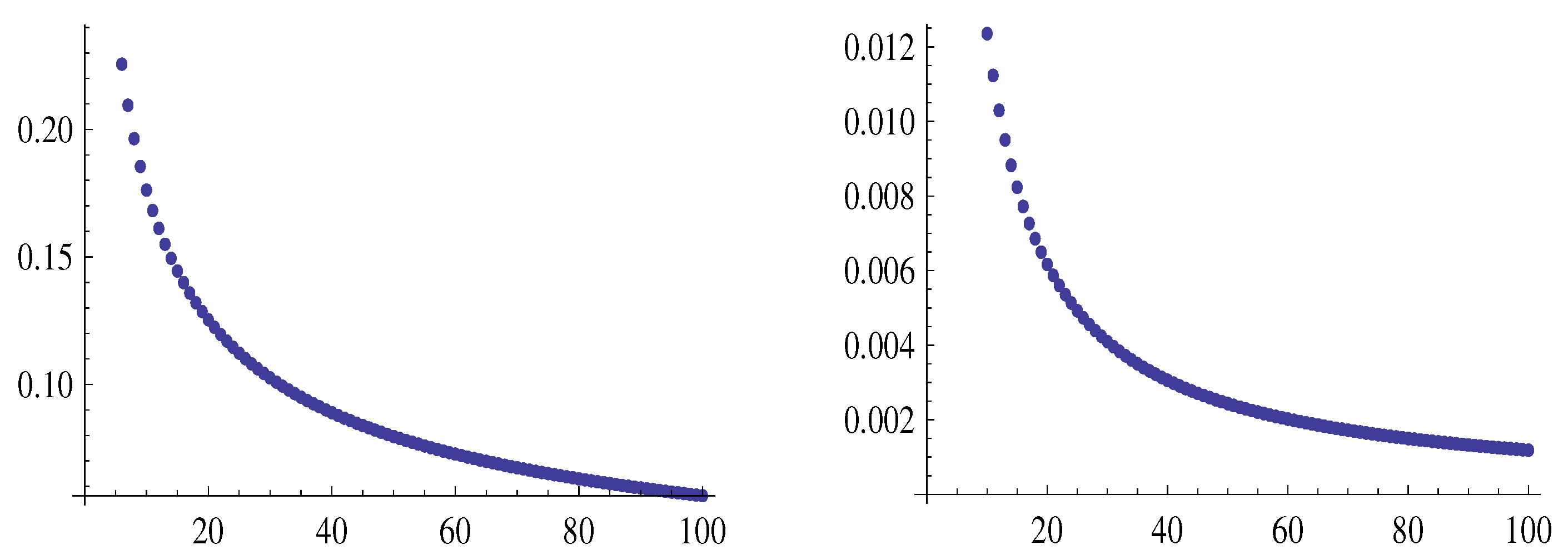
Figure 9.
The graphs of the sequences and , left and right respectively.
Disclaimer/Publisher’s Note: The statements, opinions and data contained in all publications are solely those of the individual author(s) and contributor(s) and not of MDPI and/or the editor(s). MDPI and/or the editor(s) disclaim responsibility for any injury to people or property resulting from any ideas, methods, instructions or products referred to in the content. |
© 2024 by the authors. Licensee MDPI, Basel, Switzerland. This article is an open access article distributed under the terms and conditions of the Creative Commons Attribution (CC BY) license (http://creativecommons.org/licenses/by/4.0/).
Copyright: This open access article is published under a Creative Commons CC BY 4.0 license, which permit the free download, distribution, and reuse, provided that the author and preprint are cited in any reuse.


