Preprint
Article

This version is not peer-reviewed.

Object Detection Post-Processing Accelerator Based on Co-Design of Hardware and Software

A peer-reviewed article of this preprint also exists.

Submitted:

04 December 2024

Posted:

05 December 2024

You are already at the latest version

Abstract

Deep learning significantly advances object detection. Post process, a critical component of this process, selects valid bounding boxes to represent true targets during inference and assigns boxes and labels to these objects during training to optimize the loss function. However, post process constitutes a substantial portion of the total processing time for a single image. This inefficiency primarily arises from the extensive Intersection over Union (IoU) calculations required between numerous redundant bounding boxes in post-processing algorithms. To reduce the redundant IoU calculations, we introduce a classification prioritization strategy during both training and inference post processes. Additionally, post process involves sorting operations that contribute to inefficiency. To minimize unnecessary comparisons in Top-K sorting, we have improved the bitonic sorter by developing a hybrid bitonic algorithm. These improvements have effectively accelerated post process. Given the similarities between training and inference post processes, we unify four typical post-processing algorithms and design a hardware accelerator based on this framework. Our accelerator achieves at least 7.55 times the speed in inference post process compared to recent accelerators. When compared to the RTX 2080 Ti system, our proposed accelerator offers at least 21.93 times the speed for training post process and 19.89 times for inference post process, thereby significantly enhancing the efficiency of loss function minimization.

Keywords: 
;  ;  ;  

1. Introduction

Object detection, a fundamental task in deep learning, has found widespread application in fields such as autonomous driving [1,2], agricultural monitoring [3,4], and geological exploration [5,6]. The complete training process for object detection includes feature extraction through the backbone [7,8], feature fusion via the neck [9,10], detection heads [11,12,13], post process [14], loss calculation [12,13,15,16], and back propagation. During inference, the step of loss calculation is omitted. The backbone, neck, and head are typically implemented using Convolutional Neural Networks (CNNs). Post process mainly selects valid bounding boxes. In the training phase, post process is responsible for assigning labels to the bounding boxes produced by the detection head. This step involves matching detected bounding boxes with ground truth targets and is commonly referred to as Label Assignment (LA). During the inference phase, post process involves choosing bounding boxes that represent true targets using Non Maximum Suppression (NMS).
As shown in Figure 1, Figure 1(a) illustrates the inference post process of NMS, which selects the most suitable bounding boxes to represent true targets based on the IoU threshold and confidence sorting. Figure 1(a) shows NMS excluding box1 and box3, and selecting box2 as the most appropriate bounding box to represent the true target. Figure 1(b) illustrates the training post process, namely Label Assignment (LA), with Faster-RCNN as an example. Figure 1(b) shows the Faster-RCNN post process, which eliminates box1 and box3, selects box2, and assigns the dog label to the ground truth (GT) target. In supervised learning, matching bounding boxes with true target boxes is crucial for improving model accuracy by optimizing classification losses and positional losses. Both NMS in inference and LA in training share the common goal of selecting the most appropriate bounding boxes to correspond with or represent true target boxes, highlighting their similarity in post-processing tasks. However, previous CNN hardware accelerators for object detection [17,18,19,20] have mainly focused on the feature processing stages, such as feature extraction through the backbone, feature fusion via the neck, and detection heads. Hardware acceleration for post process has received relatively little attention. This oversight stems from the differences in the algorithms of post process across various object detectors. For example, in the training phases of Faster-RCNN [21], YOLOv8s, and GFL [22], bounding boxes are assigned to true target boxes using Max IoU Assigner, Task Aligned Assigner [23], and Dynamic Soft Label Assigner, respectively. Compared to training post process, the pattern of inference post process is relatively singular. In inference post process, all three networks use NMS to select bounding boxes that can represent true targets. Therefore, despite the similarities between training and inference post processes, establishing a unified post processing workflow remains challenging.
In previous post-processing accelerators, NMS has been the primary focus due to its importance for edge inference tasks. However, as edge devices increasingly require more intelligent detection capabilities, they perform local fine-tuning based on real-time data collected through cameras [24,25], thus avoiding the need for cloud-based training and the complex design associated with data transmission between local and remote locations. This evolution underscores the critical need for hardware acceleration in training post process. Despite this, there has been limited research addressing hardware acceleration of training post process to date. This is because post process faces greater challenges in achieving standardization compared to feature process, and has a steeper learning curve, leading to fewer studies on accelerating post process. Our observations indicate that both training and inference post processes constitute a significant portion of the average total processing time for a single image. As shown in Figure 2, we have used an RTX 2080 Ti to measure the processing time for training and inference on images across three typical object detectors, using the COCO dataset. In these experiments, the average time dedicated to post process during training and inference accounted for 20.5% and 22.1% of the total processing time, respectively.
Post process involves a relatively small number of parameters, yet no unified approach has been developed for parameter statistics specific to post process. We propose two potential statistical approaches. Unlike feature process, where mainstream parameter statistics tools (e.g., ONNX tools) focus solely on the number of weights and biases, post process emphasizes bounding boxes, various thresholds, and empirical parameters. The number of bounding boxes, which depends on the size of the input image, includes elements such as confidence scores, categories, and coordinates. The number of thresholds and empirical parameters is significantly smaller than the number of bounding boxes. The first approach for post process includes all bounding box coordinates, categories, and confidence scores, along with thresholds and empirical parameters. During training, it also incorporates the coordinates and categories of true target boxes. The second approach focuses solely on thresholds and empirical parameters, including true target box coordinates and categories during training, which aligns with the parameter scope used in feature process. As illustrated in Figure 3, if post process accounts for the size of feature maps (denoted as Label Assignment with Picture and Non Maximum Suppression with Picture), the total parameters for feature process are 2.28 times to 4.92 times those for post process. Conversely, if post process disregards the feature map size (represented by Label Assignment and Non Maximum Suppression), the total parameters for feature process can be up to 787,000 times those for training post process and 21.4 million times those for inference post process. Given the significant disparity in parameter scale and execution time, accelerating post process becomes imperative. The primary bottleneck in post-processing acceleration is the repeated use of bounding boxes for filtering. Thus, reducing ineffective processes during filtering and maximizing data-level parallelism are critical for enhancing post process efficiency.
Reducing redundancy in post process primarily involves minimizing unnecessary IoU calculations and superfluous comparisons.
  • Minimizing Redundant IoU Calculations: Traditional post-processing methods often involve redundant IoU calculations between redundant bounding boxes. To address this, we introduce priority of confidence threshold checking combined with classification (CTC-C) into NMS, effectively reducing the computation of ineffective IoUs. Given the operational similarities between inference post process and training post process, we also implement priority of confidence threshold checking combined with classification (CTC-C) in the training post process of Faster-RCNN. For YOLOv8s and GFL, we incorporate priority of center point position checking combined with classification (CPC-C) to further reduce redundant IoU calculations. We propose a unified algorithmic framework for these four common post-processing methods and present a design for a corresponding hardware accelerator.
  • Reducing Redundant Comparisons: Traditional Top-K element selection methods often involve full sorting, which introduces unnecessary comparisons among non-essential elements. To overcome this, we introduce the hybrid bitonic sorter, which avoids redundant comparisons. We detail the algorithm and hardware design of the hybrid bitonic sorter, which efficiently performs IoU sorting for bounding boxes and rapidly identifies the Top-K elements, thereby optimizing the selection of the best bounding boxes during training post process.
Efforts to leverage parallelism in post process can be categorized into two main approaches: data-level parallelism computing with categories and parallel sorting.
  • Data-level Parallelism Computing with Categories: By applying principles such as priority of CTC-C and CPC-C, we can determine the category of each bounding box prior to IoU calculation. This allows for simultaneous and independent execution of IoU computations and subsequent operations across different categories.
  • Parallel Sorting: We incorporate bitonic sorting to facilitate parallel comparisons. Unlike sorting algorithms with limited parallelism, bitonic sorting offers significantly higher efficiency and speed.
The strategy of data-level parallelism outlined above is implemented in hardware through the design of multiple parallel computation units. The contributions of this paper are summarized as follows:
  • Significance of Post Processing Software-Hardware Acceleration: This paper explores the critical importance of hardware acceleration in both training and inference post processing phases. We propose a co-design strategy that integrates both software and hardware to enhance the efficiency of post process.
  • Unified Algorithm Framework and Hardware Design: We analyze the feasibility of unifying the algorithms for training and inference post processes and present a hardware designing framework based on a unified algorithmic workflow. The accelerator achieves a minimum speedup of 7.55 times for NMS acceleration compared to recent accelerators. When evaluated solely through IP simulation, our design demonstrates superior acceleration performance relative to the number of bounding boxes. Compared to the RTX 2080 Ti system, our solution provides a minimum speedup of 21.93 times for training post process and 19.89 times for inference post process.
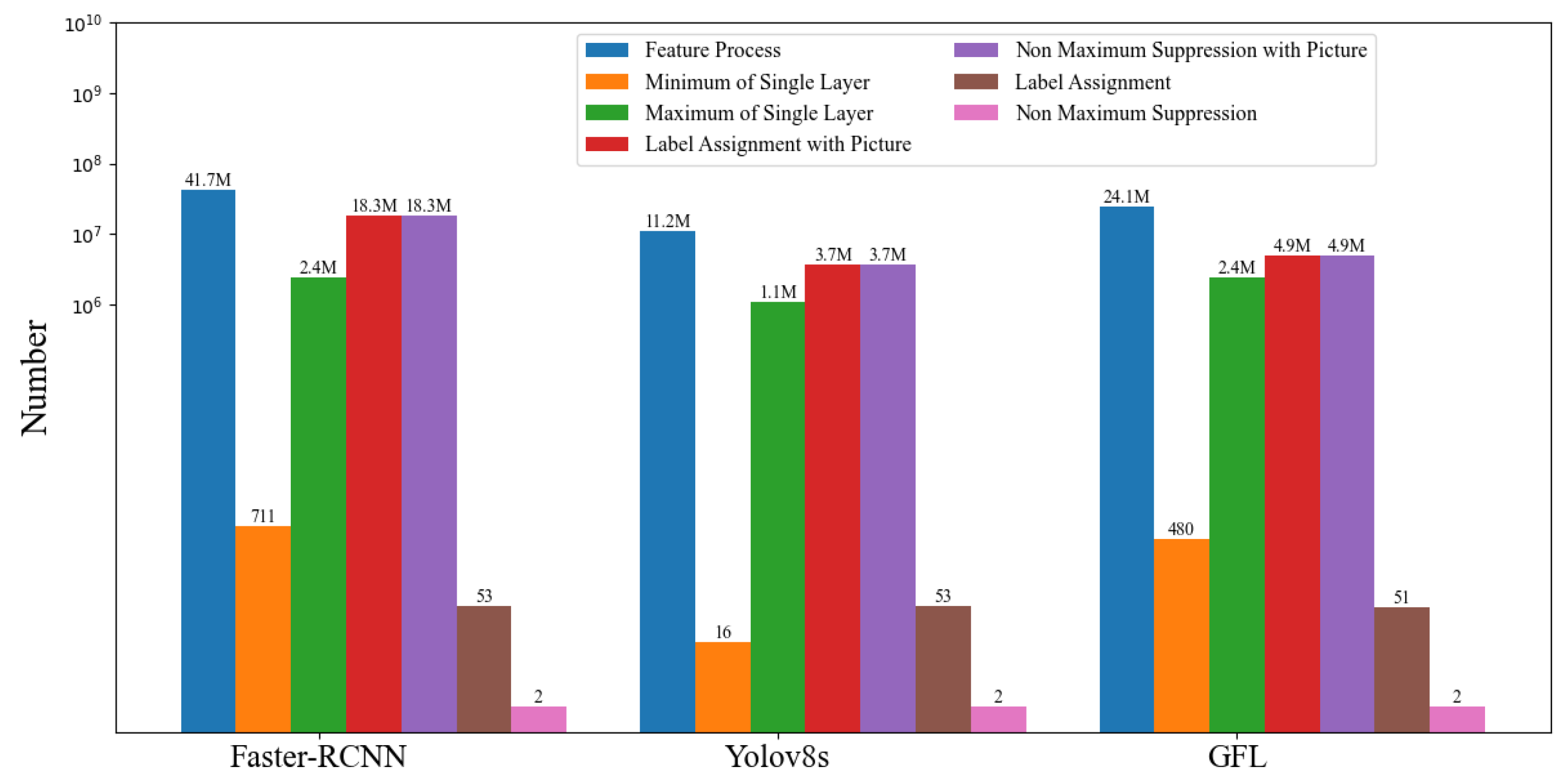
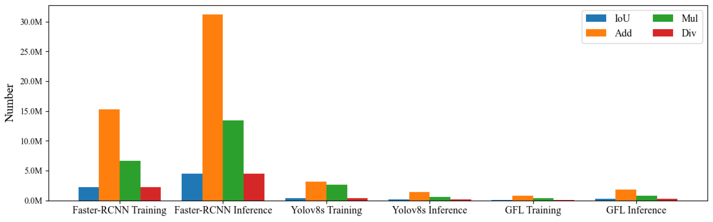
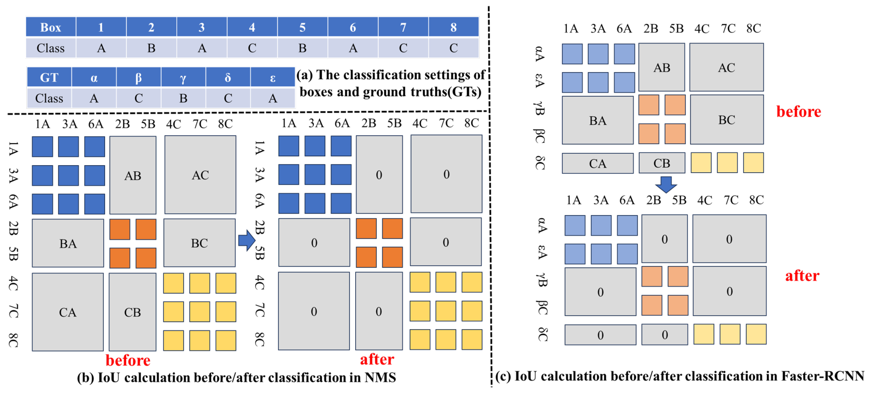
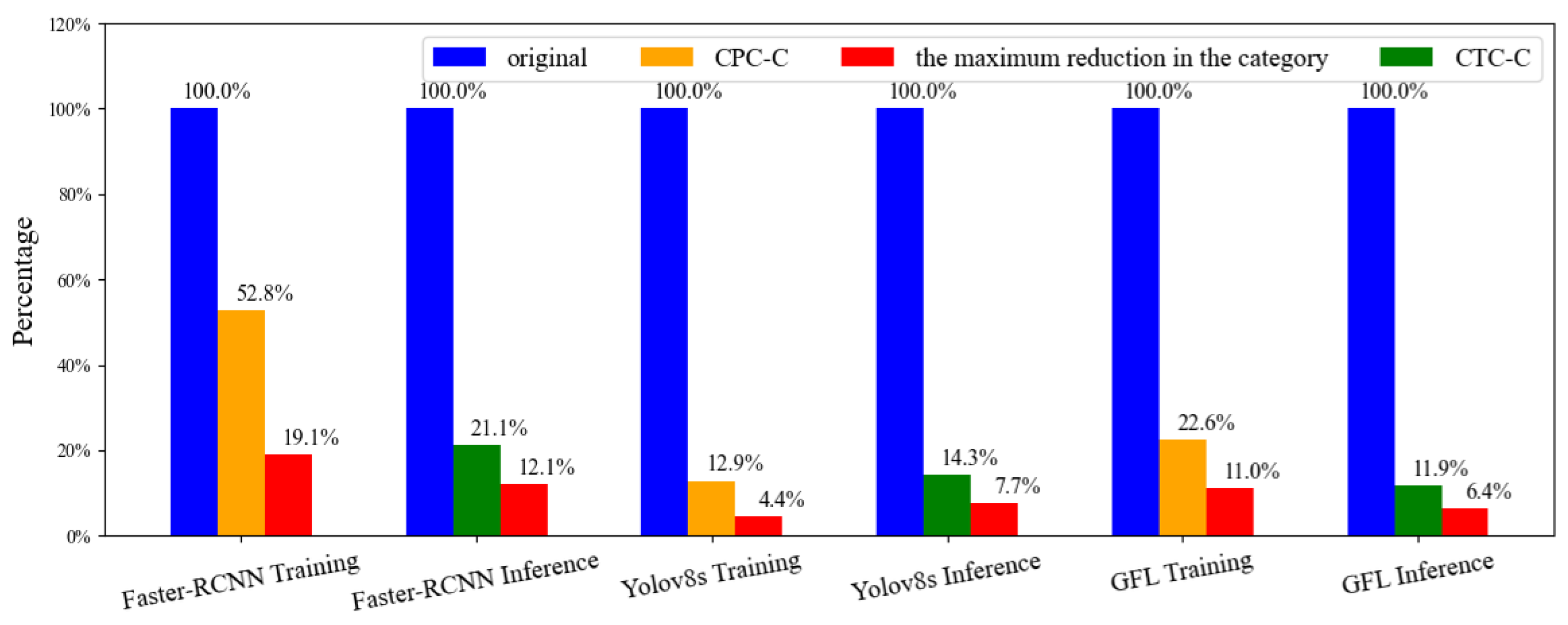
  • Reduction of Redundant IoU Calculations: We address the issue of redundant IoU calculations in training and inference post-processing algorithms. By introducing priority of CTC-C in NMS and Faster-RCNN training post process, as well as CPC-C in YOLOv8s and GFL training post process, we effectively reduce the computation of ineffective IoUs. This reduction improves algorithmic efficiency and supports effective software and hardware co-design. With the application of bounding box center point position checking (CPC) and confidence threshold checking (CTC), the number of bounding boxes is reduced to 12.9% and 11.9% of the original count, respectively. Classification further limits the number of maximum bounding boxes per class to 4.4%–19.1% of the original. These reductions validate the effectiveness of our approach, achieving a maximum speedup of 1.19 times and a minimum of 1.10 times.
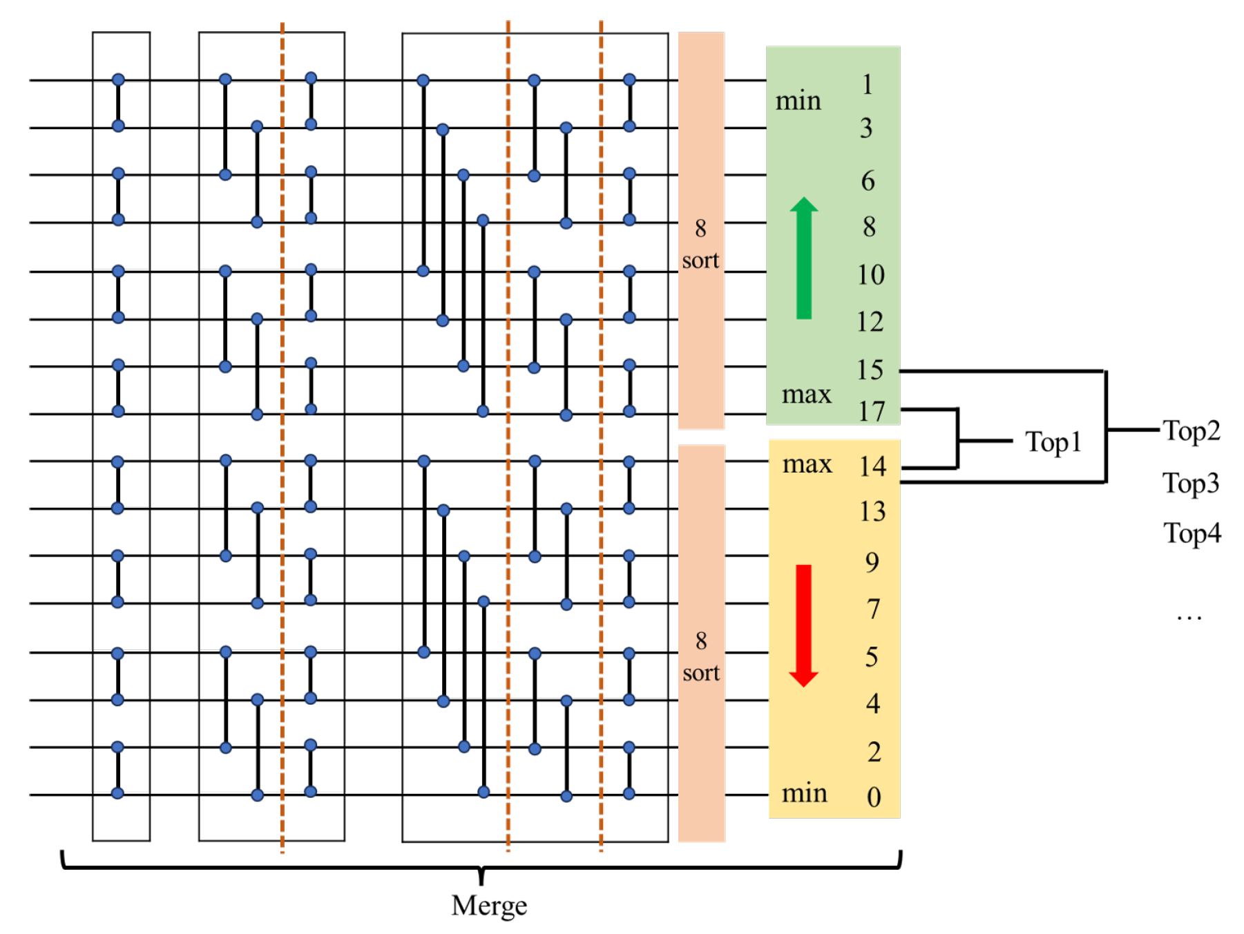
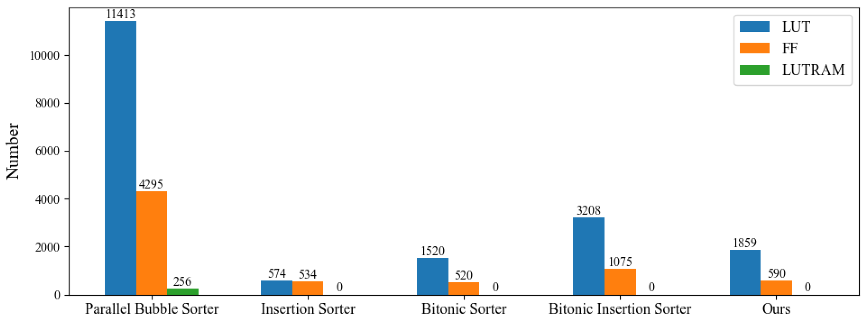
  • Design of Hybrid Bitonic Sorter: We introduce the hybrid bitonic sorter algorithm and its hardware implementation. The bitonic sorter enables highly parallel comparisons, and the Top-K algorithm within the hybrid sorter maintains this parallelism, reducing redundant comparisons typical in traditional Top-K element selection. This enhancement in sorting algorithm efficiency results in a more effective hardware solution, achieving high-performance co-design for both full sorting and Top-K sorting. Our design provides a maximum speedup of 1.25 times and a minimum of 1.05 times compared to recent sorters.

2. The Related Works

2.1. Object Detection and Post Process Algorithm

Traditional object detectors, characterized by their complex handcrafted features, generally lower accuracy, and difficulties in achieving end-to-end integration [26], are increasingly being supplanted by deep learning-based models. These modern approaches utilize network architectures with parameters scaling up to hundreds of megabytes [27,28], enabling extensive learning of object features without manual intervention. By leveraging deep networks, these models provide end-to-end object detection solutions that integrate image processing, feature learning, object classification, and localization in a unified framework.
Object detectors are classified into one-stage [29,30] and two-stage [21,31] detectors. One-stage detectors directly regress boxes in images, while two-stage detectors, although typically slower, first generate candidate regions and subsequently classify and refine these regions. Despite their slower processing speed, two-stage detectors often achieve higher detection accuracy. However, recent advancements, such as anchor-free methods[32,33,34] replacing anchor-based approaches[29,30], improved neck architectures that effectively fuse shallow and deep features[19,27], and adaptive post-processing algorithms that dynamically filter bounding boxes instead of relying on fixed empirical parameters, have led to a gradual increase in the detection accuracy of one-stage detectors. Due to their faster detection speeds, improved accuracy, and lighter models, one-stage detectors have become increasingly prevalent in applications such as intelligent transportation [35] and fire detection [36].
Post-processing algorithms in object detection can be divided into training post process and inference post process. The primary aim of training post process is to categorize samples into positive and negative classes, compute the loss between these samples and the ground truth boxes, and guide the model’s learning process based on supervisory signals. Label assignment is a key component of training post process. Label assignment methods are categorized into static and dynamic types, depending on whether thresholds for positive and negative samples vary. Static label assignment methods use fixed thresholds based on prior knowledge, such as distance and IoU, to differentiate between positive and negative samples. Examples of static methods include FCOS[37], the Max IoU Assigner in Faster-RCNN [21], and RFLA[38]. Conversely, dynamic label assignment methods adjust thresholds dynamically according to various strategies. These include ATSS[14], PAA[39], OTA[40], Dynamic Soft Label Assigner[22], SimOTA[41], and Task Align Assigner[23]. Among these, ATSS considers only dynamic IoU thresholds, while OTA, SimOTA, Dynamic Soft Label Assigner, and Task Align Assigner use joint scores of classification predictions and IoU to align the training and inference post processes. This approach results in more significant accuracy improvements compared to ATSS. Transitioning from the Max IoU Assigner to the Task Align Assigner reduces the reliance on empirical parameters and manual intervention, thereby enhancing the model’s generalizability. Despite these advancements, post process remains complex. Recent approaches have sought to simplify training post process. For instance, the Transformer-based DETR [15,42,43] end-to-end detector employs one-to-one Hungarian matching instead of one-to-many training post process. However, other Transformer-based visual detectors[44,45], such as those using the Swin Transformer[7], still utilize one-to-many training post process and achieve higher accuracy and faster convergence than DETR. Notably, although DETR claims to eliminate complex post process, NMS remains necessary during inference to filter bounding boxes. Consequently, it is expected that one-to-many training post process, which minimizes manual parameters, will continue to be the dominant approach in visual detectors for the foreseeable future.
In contrast to training post process, which has seen significant evolution, inference post process has developed more incrementally, with most advancements focusing on the IoU calculation paradigm [46,47,48,49]. Standard NMS remains the predominant technique, and thus this work employs standard NMS. NMS is a critical post process for eliminating redundant bounding boxes surrounding true targets. The standard NMS approach [50] ranks candidate bounding boxes by their confidence scores and iteratively removes those that overlap significantly with higher-IoU candidates. While standard NMS uses fixed empirical thresholds, it does not adapt to the unique characteristics of each input image, which can constrain the detector’s performance on testing datasets and lead to suboptimal detection results. To overcome this limitation, some research has redefined the selection of NMS thresholds as a convex optimization problem and applied various swarm intelligence optimization algorithms to identify the optimal solution to this problem [51]. Furthermore, adaptive NMS strategies that rely on specific complexity metrics have been developed for crowded scenarios, such as pedestrian and vehicle detection [52,53]. Despite these innovations, methods that aim to eliminate the need for NMS by improving network architectures (i.e., NMS-free mechanisms) [54,55,56] often exhibit lower performance in practical applications compared to detectors that utilize NMS.
In this paper, we focus on the latest advancements in label assignment algorithms, selecting both the Dynamic Soft Label Assigner and the Task Align Assigner. While both are derived from the paradigms established by OTA and SimOTA, they exhibit notable algorithmic differences. Additionally, we use the Max IoU Assigner from Faster-RCNN as a representative of static label assignment methods. For inference post process, we retain the standard NMS as our experimental approach.

2.2. The Hardware Accelerator in Inference Post-Processing Algorithms

Due to the extensive range of applications for object detection at the edge, hardware accelerators for inference post process garner significant attention. NMS is a critical step in this process. It involves selecting the bounding box with the highest confidence score, computing the IoU between this selected box and the remaining boxes, and then filtering out boxes that have an IoU above a specified threshold. This process of selecting the highest confidence box, computing IoU, and filtering continues iteratively until no boxes remain.
Due to the computational complexity of IoU calculation, requiring three multiplications and one division per comparison, with each bounding box needing to compute IoU with every other box, significant power consumption and hardware resource usage are incurred. To address this challenge, approximations of IoU can be employed to replace multiplications and divisions with additions and shifts, thereby reducing power consumption and hardware demands. For example, Shi et al. [57] approximate IoU by calculating the maximum values between coordinates, while Fang et al. [58] introduce additional boundary constraints to effectively eliminate the division step in IoU computation. However, these approximation methods often result in sacrifice with reduced model accuracy.
Due to the loss of model accuracy under IoU approximation, another approach is to enhance the NMS algorithm to minimize redundant calculations and leverage parallelism without loss of model accuracy. Shi et al. [57] improve NMS by employing a sliding window technique on a graph to cluster bounding boxes based on coordinate information. Their revised NMS algorithm decomposes the process into filtering within multiple bounding box clusters and uses position-based bitmap techniques to reduce ineffective data access. This approach lowers memory access and power consumption. Despite its effectiveness in evaluating similar bounding boxes through coordinate information, partitioning bounding box clusters remains challenging, particularly in dense scenarios such as face detection. Chen et al. [59] advance NMS by routing bounding boxes to three separate branches of the output head, each designed for a different ratio, and calculating the regression with maximum confidence for each branch. After merging these branches, the most suitable bounding box is selected. This method enhances parallelism up to three branches and decreases IoU calculations between bounding boxes across different branches. However, for both anchor-based and anchor-free methods, the varying number of anchors and points between different ratios makes it difficult to consistently maintain parallelism at three. Choi et al. [60] significantly improve NMS by introducing a fixed limit on the number of valid bounding boxes involved in each IoU calculation. While this modification reduces redundant calculations, the fixed limit on valid bounding boxes reduces the algorithm’s adaptability in detecting target boxes.
Furthermore, optimizing the NMS by maintaining its core principles while utilizing its threshold parameters to mitigate IoU redundancy represents another strategy for improving algorithm performance. Research [61,62,63,64] shows that applying confidence thresholds to filter out unsuitable bounding boxes can significantly reduce the number of boxes involved in IoU calculations. Anupreetham et al. [65] innovate by adapting the NMS approach for SSD detectors. Instead of the traditional method of waiting to process all bounding boxes and then selecting the one with the highest confidence, their approach employs a pipelined system where boxes are sequentially fed into the computation engine. They introduce three criteria for bounding box selection: whether the box belongs to the same class, whether its IoU exceeds a threshold, and whether its confidence is greater than that of the currently occupied box. This approach is distinguished by its incorporation of class information into the bounding box selection process, unlike the method proposed by Shi et al. [57], which focused solely on coordinate-based clustering and did not address the distribution of different classes within the same spatial region. However, despite [65] integrating class information into the selection process, Anupreetham et al.’s approach does not apply class information to the exclusion of IoU redundancy.
This work introduces an approach that prioritizes both class information and confidence thresholds checking to significantly reduce IoU calculations between bounding boxes of different classes before performing the IoU computation. Table 1 provides a detailed comparison of recent studies highlighting these differences.

2.3. The Hardware Accelerator in Sorter Algorithm

Due to the necessity of sorting by confidence scores and IoU in NMS, as well as the requirement for Top-K selection of alignment scores in both the Dynamic Soft Label Assigner and Task Aligned Assigner, efficient sorting techniques are critical. Fang et al. [58] address the storage challenges associated with sorting operations by using a comparator tree, which reduces the storage demands by efficiently managing sorted elements, given that NMS focuses only on the maximum confidence value in each iteration. Meanwhile, Sun et al. [64] employ parallel bitonic sorting to order IoU values between bounding boxes.
Bitonic sorting [66], in contrast to traditional bubble sorting, provides faster sorting through parallel comparisons. Bitonic sorting involves two phases: In the merge phase, input elements are organized into bitonic sequences that include both ascending and descending subsequences. At the end of this phase, two subsequences of elements each are created, corresponding to ascending and descending orders. The subsequent sort phase involves recursively subdividing these subsequences until each is reduced to a length of one.
Although this approach improves efficiency, hardware implementation incurs higher costs with increasing numbers of elements N due to the necessity of multiple comparators. To address this issue, Chen et al. [67] avoid further recursion after the merge phase by using dual insertion sorting, which reduces resource consumption. Zhao et al. [68] extend the bitonic sorting concept by introducing a smaller merge sort after the merge phase to facilitate Top-K extraction, specifically for K=2. Alternatively, Fang et al. [69] use insertion sorting to identify Top-K elements, but this method is constrained by the sorting scale and longer delays.
In line with the hybrid bitonic sorting methods proposed by [67,68], our work introduces a hybrid bitonic sorting that supports both full sorting and Top-K extraction. However, our method differs by incorporating multi-comparator trees during the merge phase to directly obtain Top-K elements, instead of the traditional approach that only identifies the maximum value. Additionally, we overcome the K=2 limitation present in previous methods, enabling greater parallelism due to the parallelizable nature of retrieving K elements. Table 2 presents the sorting schemes of recent sorting accelerators and provides a comparison.

3. The Unification of Post Process Algorithm and Optimization

3.1. Analysis of the Uniformity of Post-Processing Algorithms

In Faster-RCNN, the Max IoU Assigner begins by filtering out unsuitable bounding boxes based on a confidence threshold. It then calculates the IoU between the remaining bounding boxes and the ground truth boxes, selecting the bounding boxes that match the ground truth boxes according to predefined thresholds. Similarly, in Yolov8s, the Task Align Assigner and GFL’s Dynamic Soft Label Assigner first eliminate unsuitable bounding boxes based on whether their center points fall within the ground truth boxes. They then compute alignment scores for each bounding box by combining classification scores and IoUs. The Task Align Assigner assigns a fixed number of bounding boxes for each ground truth target, whereas the Dynamic Soft Label Assigner adaptively determines the number of bounding boxes by selecting and summing the top-K alignment scores for each ground truth target, making it more flexible.
For NMS, the process starts by selecting the bounding box with the highest confidence score from all candidate boxes. The IoU is then calculated between this highest-confidence box and the remaining boxes. Bounding boxes with an IoU exceeding a predefined threshold are removed. This process of selecting the highest-confidence box and recalculating IoU is repeated until no bounding boxes remain.
From a procedural standpoint, as illustrated in Figure 4, we categorize the workflow into four stages: Pre-Process, Alignment, Dynamic Sampling, and Sorter:
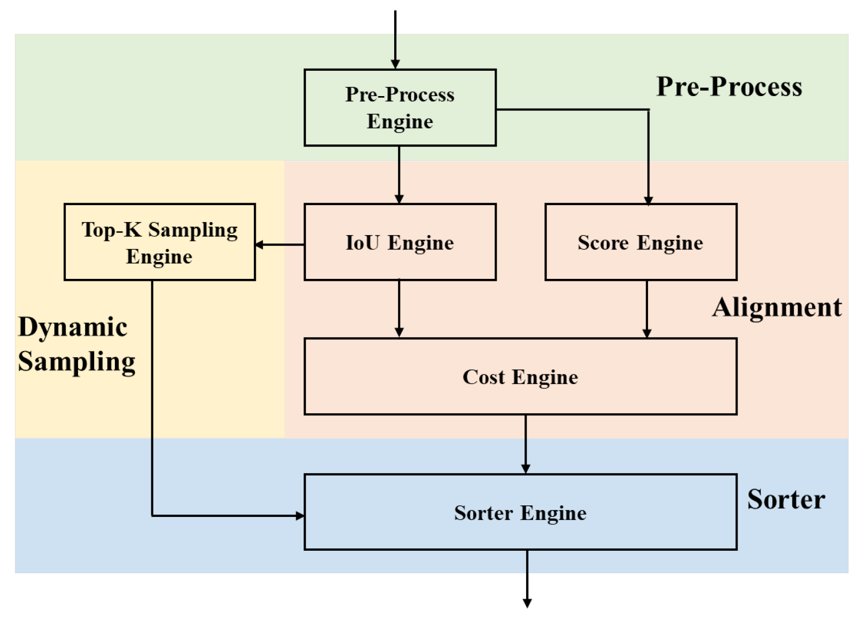
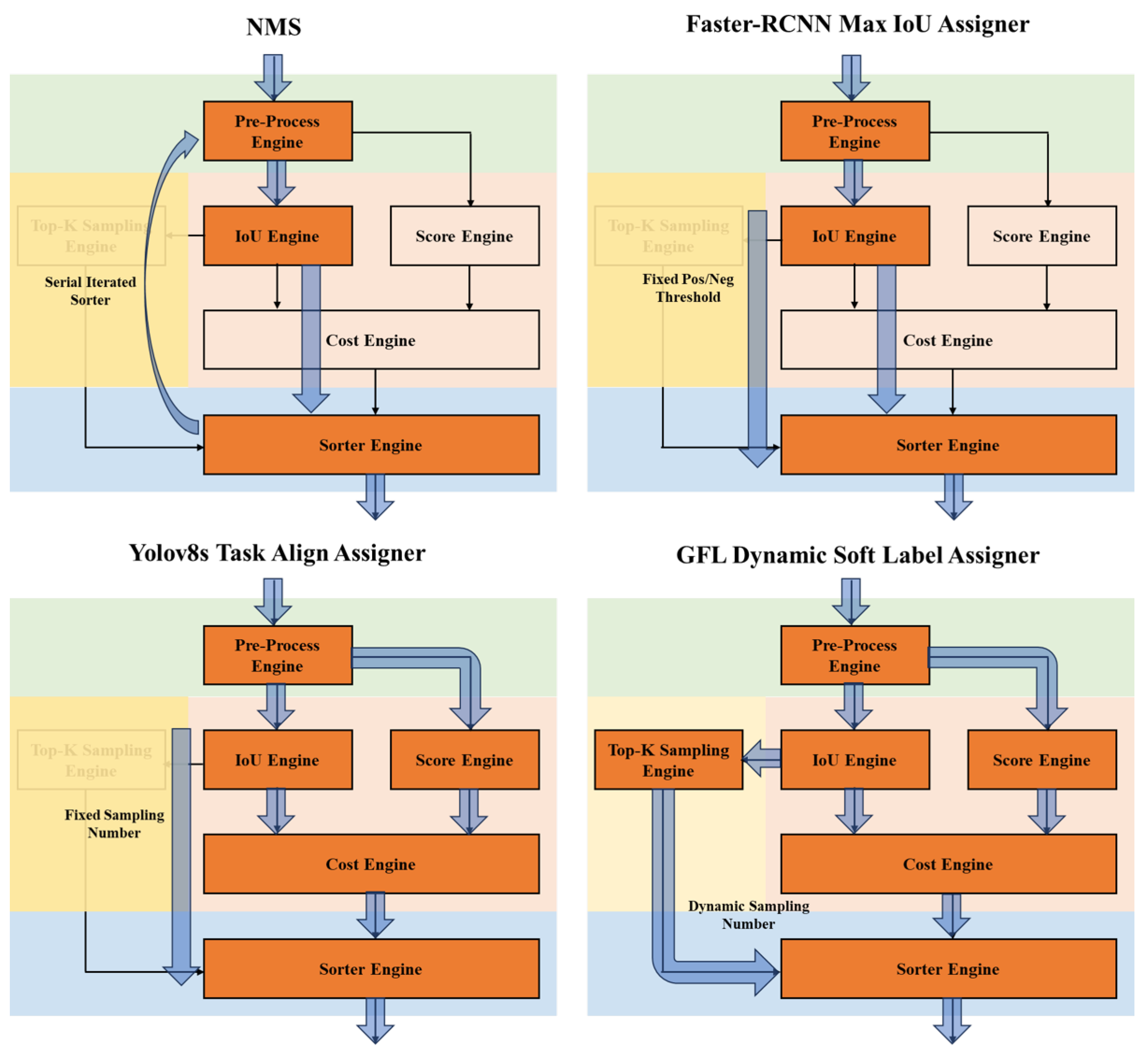
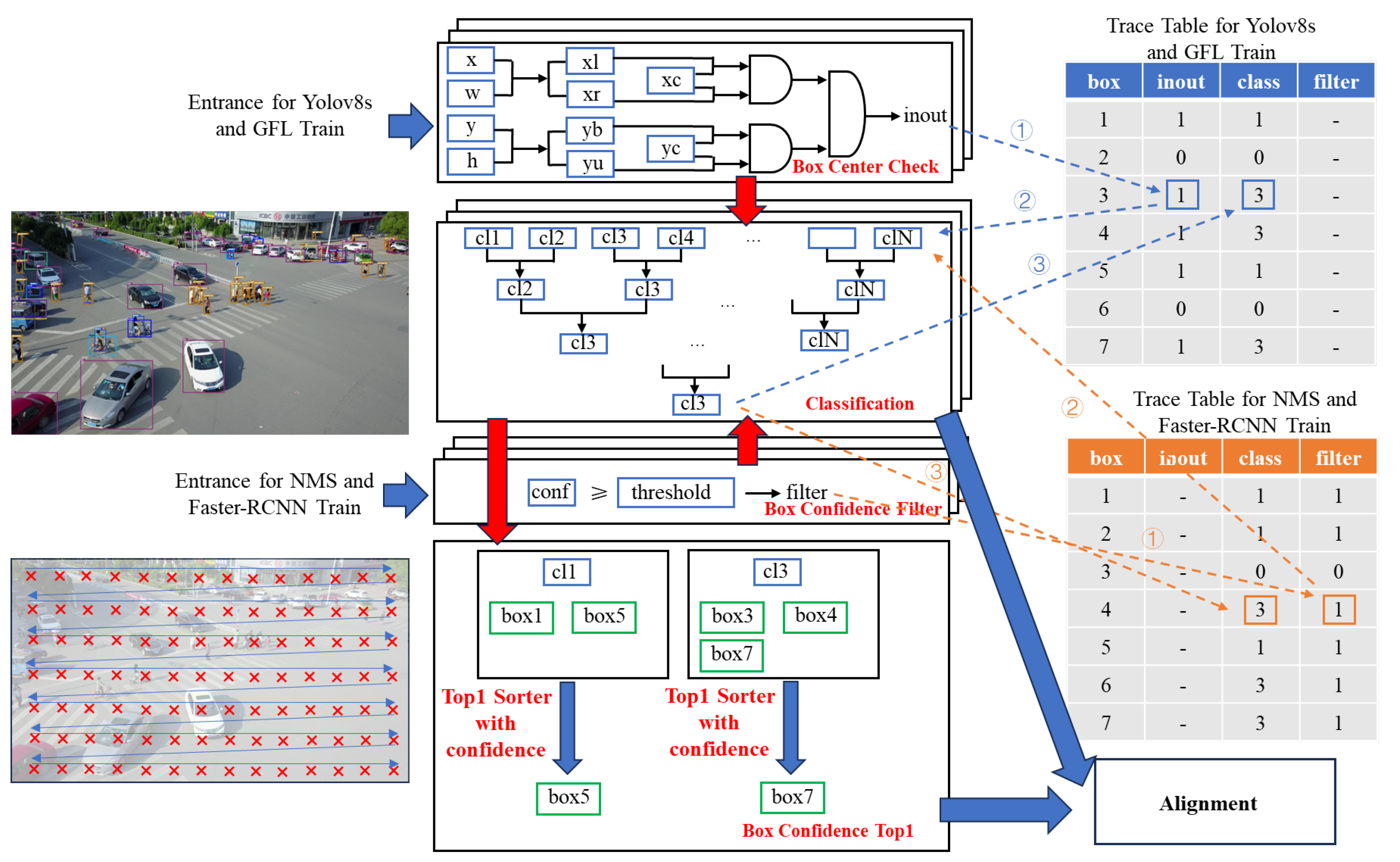
  • Step 1. Pre-Process: This step involves extracting the bounding box with the highest confidence or verifying whether the bounding box center point is within the ground truth boxes. To be detailed, as shown in Figure 4, the light green background represents the Pre-Process stage, where the input is data related to bounding boxes, and the output is qualified bounding boxes that have undergone classification, confidence judgment, and center determination of the bounding box. The core element is the Pre-Process Engine.
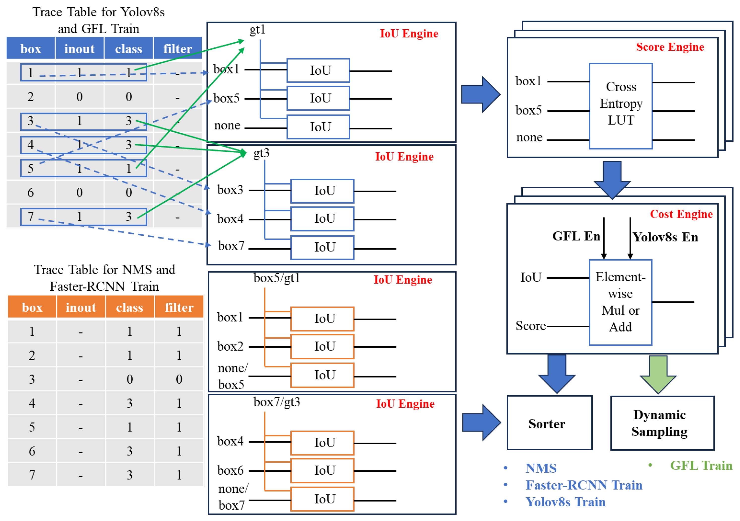
  • Step 2. Alignment: This step calculates the IoU between the bounding boxes and the ground truth. Both the Task Align Assigner and the Dynamic Soft Label Assigner additionally compute alignment scores by integrating classification values with IoU. As shown in Figure 4, the light pink background represents the Alignment stage, where the input includes the coordinate and category information of qualified bounding boxes, as well as the coordinate and category information of ground truth. Possible outputs include the IoU matrix and alignment score matrix constructed based on qualified bounding boxes and ground truth. The core elements are the IoU Engine, Score Engine, and Cost Engine, with the IoU Engine responsible for calculating the IoU matrix, the Score Engine responsible for calculating the classification score matrix, and the Cost Engine responsible for calculating the alignment score matrix.
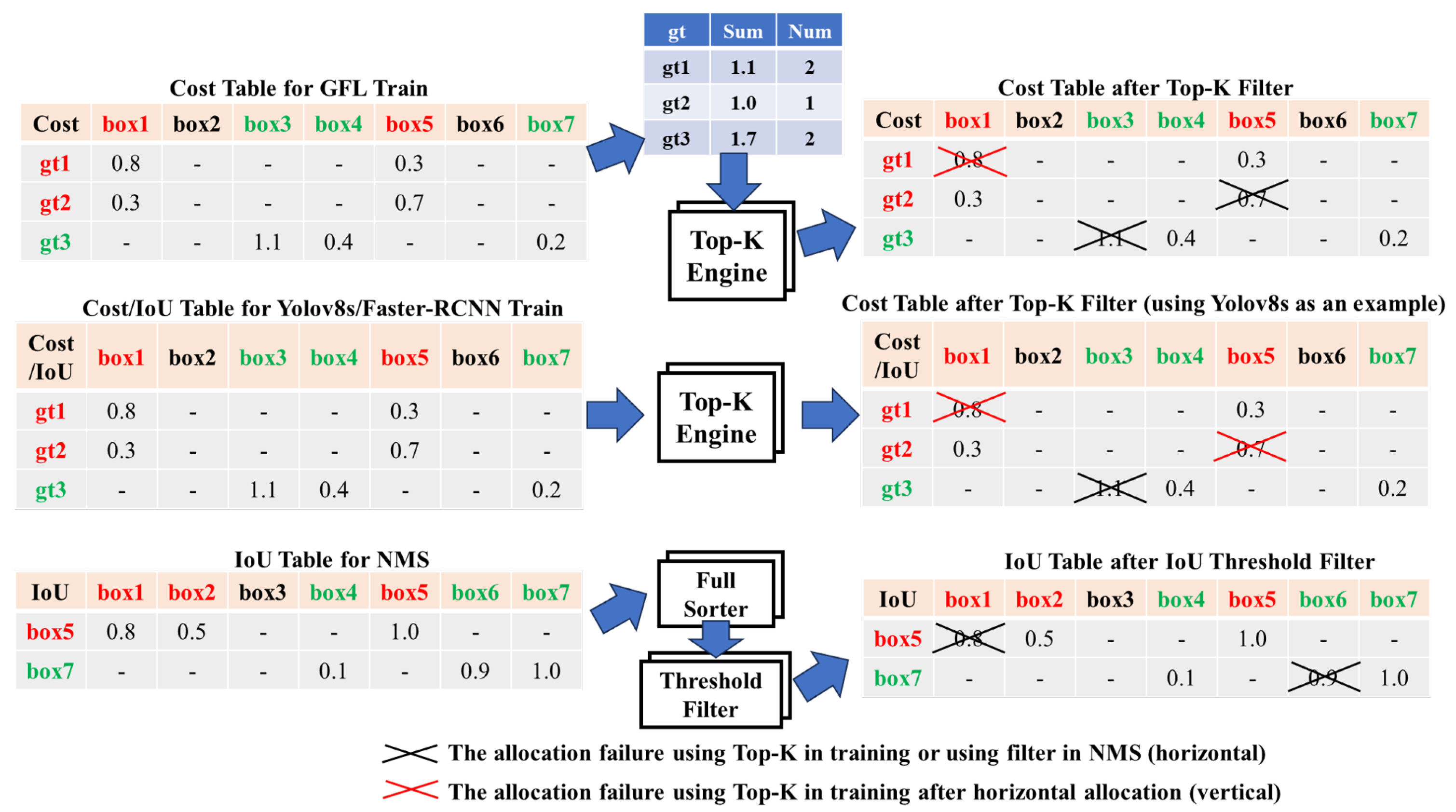
  • Step 3. Dynamic Sampling: This step determines the number of bounding boxes corresponding to each ground truth target, a requirement specific to the Dynamic Soft Label Assigner based on its alignment scores. In Figure 4, the light yellow background represents the Dynamic Sampling stage, where the input is the alignment score matrix, and the output is the maximum number of bounding boxes that each ground truth can be assigned to. The core element is the Top-K Sampling Engine, used only for Dynamic Soft Label Assigner.
  • Step 4. Sorter: This final step involves sorting and selecting bounding boxes based on IoU matrix or alignment score matrix. In Figure 4, the light blue background represents the Sorter stage, where possible inputs include the IoU matrix, alignment score matrix, and the number of bounding boxes that each ground truth can be assigned to, with the output being the assignment of bounding boxes to each ground truth or true target.
Figure 5 illustrates the re-expression of the four types of algorithms within a unified workflow. The orange boxes highlight the enabled steps, while the light blue arrows indicate the flow of data.
  • NMS: In the Pre-Process stage, NMS identifies the bounding box with the highest confidence score. During the Alignment stage, it calculates the IoU between the selected bounding box and the remaining ones. In the Sorter stage, IoUs are sorted, and bounding boxes are filtered based on predefined IoU thresholds. This iterative process continues until no bounding boxes remain.
  • Max IoU Assigner: This algorithm filters bounding boxes based on confidence in the Pre-Process stage. It then computes the IoU matrix between bounding boxes and ground truth boxes in the Alignment stage. In the Sorter stage, IoUs are sorted and used to filter bounding boxes according to IoU thresholds, mapping each bounding box to its corresponding ground truth box.
  • Task Align Assigner: In the Pre-Process stage, this algorithm filters bounding boxes based on confidence. The Alignment stage involves calculating IoU matrix and alignment score matrix. During the Sorter stage, alignment scores are sorted, and bounding boxes are selected based on a fixed number of boxes per ground truth target, mapping them accordingly.
  • Dynamic Soft Label Assigner: This method filters bounding boxes based on confidence in the Pre-Process stage. It calculates IoU matrix and alignment score matrix, using both classification and IoU, during the Alignment stage. The number of allowable bounding boxes per ground truth target is determined based on alignment scores in Dynamic Sampling stage. In the Sorter stage, alignment scores are sorted, and bounding boxes are selected according to the number required for each ground truth target, effectively mapping them to the ground truth boxes.
Based on our analysis of post-processing algorithms, we propose a unified algorithmic workflow. By investigating the implementation details and characteristics of each algorithm, we examine their specific functionalities within this unified framework. This approach establishes a solid foundation for hardware design.

3.2. Redundancy Analysis of Post-Processing Algorithms

Both training and inference post processes involve extensive IoU calculations. The IoU calculation involves computing the areas of two bounding boxes, A and B, and their overlapping region. The IoU is then defined as the ratio of the overlapping area to the total area covered by both bounding boxes, as expressed by Equation 1. Here, Equation 2 calculates the area S A of A based on the width w A and height h A of A, Equation 3 calculates the area S B of B based on the width w B and height h B of B, and Equation 4 marks the overlapping area of A and B as S cross . Each IoU calculation requires three multiplications and one division. Consequently, optimizing the IoU calculation is crucial for efficiency. Unlike the methods proposed in [57,58], which simplify the IoU calculation to reduce the number of multiplications and divisions, our approach retains the standard IoU computation. This choice ensures the accuracy of alignment scores and maintains the algorithm’s generalizability in training post process.
IoU = S cross S A + S B S cross
S A = w A × h A
S B = w B × h B
S cross = S A S B
In post-processing algorithms, IoU calculations are performed either between different bounding boxes or between bounding boxes and ground truth boxes. As depicted in Figure 6, the volume of such IoU calculations in post process can reach the order of millions. Given the previously discussed principles of post process, these calculations often involve redundancy. Consequently, eliminating redundant IoU calculations can significantly reduce the system’s overall power consumption and improve its acceleration efficiency.
In standard post-processing algorithms, a substantial number of IoU calculations are performed between bounding boxes of different classes or between bounding boxes and ground truth boxes of different classes. However, many of these IoU calculations do not aid in the selection process. To address this inefficiency, distinguishing bounding boxes by class through a prior classification step can be advantageous. Unlike the approach taken in [65], our method incorporates classification before performing IoU calculations. Specifically, this classification strategy is applied after confidence filtering or bounding box qualification but prior to IoU computation.

3.3. Redundancy Optimizations for Post-Processing Algorithms

Employing early classification prior to computing IoU can significantly reduce the number of redundant IoU calculations. For instance, in the inference phase, as depicted in Figure 7, the object detector’s classification head generates 8 bounding boxes, necessitating pairwise IoU calculations. This results in a total of 64 IoU computations. By incorporating early classification and limiting IoU calculations to bounding boxes of the same class, the number of required IoU computations is reduced to 22. Consequently, this approach decreases the total IoU calculations to 34.4% of the original amount. Similarly, during the training phase, if 8 bounding boxes are returned and need to be matched with 5 ground truth boxes, the number of IoU calculations would otherwise total 40. However, with early classification, this number is reduced to 13, which is 32.5% of the original number.
In contrast to [57,58], our approach, consistent with several other studies, retains confidence filtering in the NMS algorithm and preserves the bounding box center point position checking in the post-processing phase. Despite incorporating early classification, we have not modified the post-processing algorithms. Instead, we have reduced redundant calculations by leveraging early classification.

4. Accelerator Framework Design

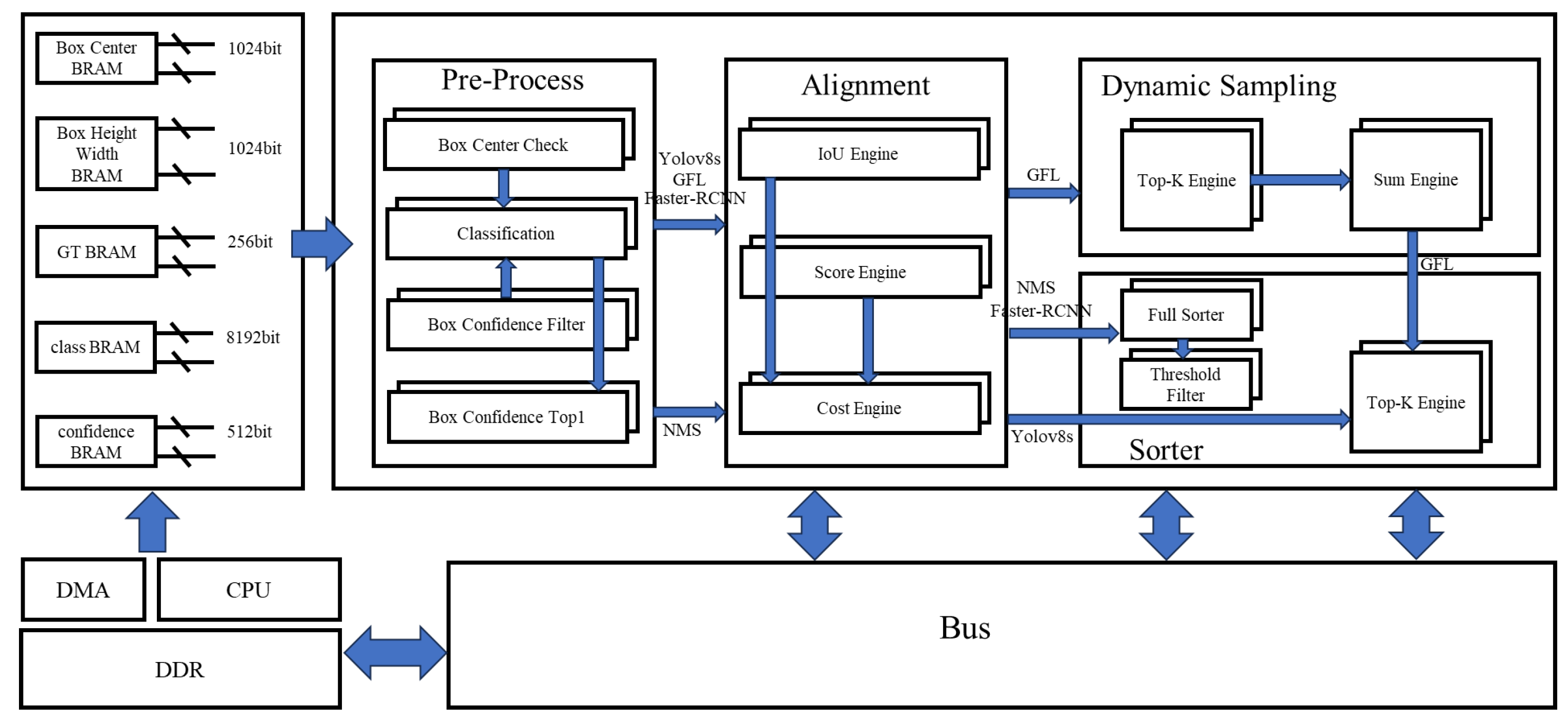
4.1. Overall Framework Design of Accelerator

Based on the previous analysis of the uniformity and redundancy in the post-processing algorithms, we identify that post processes can be effectively structured into four key stages: Pre-Process, Alignment, Dynamic Sampling, and Sorter.
We propose a hardware accelerator architecture for post processes, as illustrated in Figure 8. The system consists of a CPU for managing read/write control registers, a DMA for transferring data to BRAM, BRAM which supplies data to the accelerator IP, the post-processing accelerator IP, and a bus system for control and data transfer. The post-processing accelerator IP is designed to implement the four stages: Pre-Process, Alignment, Dynamic Sampling, and Sorter. Control signals are utilized to identify whether the algorithm is in training or inference mode. In training mode, additional differentiation is made among the Max IoU Assigner, Task Align Assigner, and Dynamic Soft Label Assigner. Data pathways are selected through enabling mechanisms, as depicted in Figure 5.
In our design, the data width is set to 8 bits, primarily because the precision loss during post process is considerably less significant compared to that in feature processing network layers. Consequently, this choice does not markedly affect the final detection accuracy, with an observed average accuracy loss of only 0.02%. We process 8 ground truth boxes and 64 bounding boxes in a single pass. The input data comprises two coordinates for each GT, center point coordinates, width and height dimensions for each bounding box, and the category data and confidence scores for each box. This data is written to the corresponding BRAM write ports via DMA, while the read ports of BRAM supply data to the post-processing accelerator IP.

4.2. The Design of Hybrid Bitonic Sorter

The Box Confidence Filter, Top-K Engine, and Full Sorter within the post-processing accelerator (shown in Figure 8) all require sorting. In this paper, we propose an innovative hybrid sorting approach based on bitonic sorters. During the merge phase of bitonic sorting, the ascending and descending subsequences can be utilized to pinpoint the maximum values. Moreover, leveraging the known order relationships within these subsequences, a comparator tree can efficiently determine the Top-2 and Top-3 maximum values. This approach allows us to replace traditional sorting phases with a comparator tree, thus minimizing unnecessary sorting operations and facilitating faster retrieval of Top-K data. Our sorter design features a fundamental unit comprising a 32-input sorter, capable of managing up to 16 Top-K elements, as demonstrated in Figure 9.

4.3. The Design of Pre-Process Submodule

As illustrated in Figure 10, bounding boxes are derived from different ratio layers centered at various points (denoted as × on the left side of Figure 10). By sliding across image frames (i.e., moving × from left to right as shown), the number of bounding boxes that need to be compared or filtered can be significantly reduced. This method is effective because a bounding box in the bottom right corner of the image is unlikely to overlap with one in the top left corner. Moreover, this approach tends to group bounding boxes near the same center point into a limited number of categories, thereby facilitating the formation of clusters of bounding boxes within the same class. We utilize this sliding technique for bounding boxes around the input center points in our approach.
In the Pre-Process submodule, the data path varies according to the algorithm type, as depicted in Figure 10. The input to the Pre-Process submodule can come from bounding box-related data in both YOLOv8s training post process and GFL training post process, as well as from NMS and Faster-RCNN training post process. For the former, the data is processed in the Box Center Check to determine if the bounding box center point lies within the ground truth box. Here, x, w, y, and h represent the x-coordinate of the ground truth center point, the ground truth’s horizontal width, the y-coordinate of the ground truth center point, and the ground truth’s vertical height, respectively. x l , x r , y b , and y u represent the left x-coordinate, right x-coordinate, bottom y-coordinate, and top y-coordinate of the ground truth, calculated based on x, w, y, and h. x c and y c represent the x-coordinate and y-coordinate of the bounding box center point, respectively. The output results are entered into the Trace Table’s inout column; for example, , where 1 indicates that the bounding box center point is within the ground truth, and 0 indicates it is not. For the latter, the bounding box confidence is filtered by the Box Confidence Filter using a confidence threshold, and the results are filled into the filter column of the Trace Table; for example, , where 1 indicates confidence above the threshold, and 0 indicates confidence below the threshold. Subsequently, all four algorithms proceed to Classification, where they are categorized using a classification tree. For example, both and send the probability of each category for qualified bounding boxes into Classification, and the results are written into the Trace Table, such as and , which record the category judgment results in the corresponding class column of the Trace Table. With this, the Pre-Process for the post processes of YOLOv8s, GFL, and Faster-RCNN training is complete, and the Trace Table can be passed on to the Alignment submodule. NMS, however, still requires sending bounding boxes of the same category to Box Confidence Top1 to obtain the bounding box with the highest confidence for each category, such as box5 and box7 being the bounding boxes with the highest confidence in the first and third categories, respectively, and then passing the identifier and Trace Table to the Alignment submodule. The Top1 Sorter with confidence still employs the classification tree.

4.4. The Design of Alignment Submodule

As shown in Figure 11, the data flow within the Alignment submodule differs based on the algorithm used. Taking the training post processes of YOLOv8s and GFL as examples, in the IoU Engine, the GT coordinates for class 1 and class 3 serve as one input for IoU calculation, while the other input comes from the coordinates of bounding boxes of the same class, thereby obtaining the IoU between the GT and the bounding boxes. Subsequently, in the Score Engine, the category of the bounding box is input to obtain the cross-entropy category score. Due to the computational complexity of the logarithmic operations in the cross-entropy function, a lookup table is utilized within the module for this calculation. Following this, in the Cost Engine, the alignment score for GFL is derived by summing the classification score and the IoU. For YOLOv8s, the alignment score is obtained by multiplying the classification score and the IoU after applying a power function with an exponent of 1, which does not significantly affect the model’s accuracy. Finally, GFL sends the alignment score to the Dynamic Sampling submodule, while YOLOv8s sends the alignment score to the Sorter submodule. In contrast, for NMS and Faster-RCNN training post process, the Score Engine and Cost Engine are not required. NMS uses the coordinates of the highest confidence bounding boxes output by the Pre-Process submodule as one input for IoU calculation, with the other input being the coordinates of other bounding boxes of the same class. Faster-RCNN, on the other hand, uses the GT coordinates for class 1 and class 3 as one input for IoU calculation, with the other input coming from the coordinates of bounding boxes of the same class, thereby obtaining the IoU between the GT and the bounding boxes. The IoU obtained from NMS and Faster-RCNN post processes through the IoU Engine is directly sent to the Sorter submodule.

4.5. The Design of Dynamic Sampling and Sorter Submodules

As shown in Figure 12, the Dynamic Sampling submodule is exclusively used for training post process in GFL. The alignment scores between each bounding box and ground truth (i.e., the Cost Table) are obtained from the Cost Engine of the Alignment submodule. These alignment scores are then processed by the Top-K Engine and Sum Engine within the Dynamic Sampling module, as shown in Figure 8, yielding the results presented in the blue table of Figure 12. The Top-K Engine first selects the top K maximum cost values between the ground truth and the bounding boxes, and then the Sum Engine calculates the Sum values for each gt in the blue table in Figure 12. For example, for gt1, the top K maximum numbers are only 0.8 and 0.3, so they sum up to 1.1, and thus the Sum for gt1 is filled with 1.1. To determine the maximum number of bounding boxes, Num, that can be assigned to each gt, the decision is made based on whether the decimal part of the fixed-point number is zero—if it is zero, the integer part is taken, such as 1.0 being taken as 1; if it is not zero, the integer part is incremented by one, such as 1.1, where the integer part is incremented by one to get 2. This result is stored in the buffer of the Dynamic Sampling submodule and subsequently passed to the Sorter submodule.
For the Sorter submodule, the inputs vary among the four types of algorithms. For GFL, the number of boxes, Num, corresponding to each gt and the Cost Table are used as inputs, with boxes being assigned to the appropriate gt through the Top-K Engine; for YOLOv8s, the Cost Table is used as input, and boxes are assigned to the appropriate gt through the Top-K Engine; for Faster-RCNN and NMS, the IoU Table is used as input. For Faster-RCNN, boxes are assigned to the appropriate gt through the Top-K Engine, while for NMS, the most suitable boxes to represent the true targets are selected through the Full Sorter and Threshold Filter. Taking GFL as an example, gt1, gt2, and gt3 are allowed to be assigned up to 2, 1, and 2 boxes, respectively. Therefore, gt1 can initially be assigned to box1 and box5, gt2 can be assigned to box1 (box5, due to its large cost value and the fact that gt2 can be assigned to at most one box, is not assigned to gt2, which is referred to as The allocation failure using Top-K in training or using filter in NMS), and gt3 can be assigned to box4 and box7. Since the same box cannot be assigned to two gts, gt1 and gt2 compete for box1. According to the principle of the smallest cost, gt2 obtains box1, and gt1 loses its box1 (this is referred to as The allocation failure using Top-K in training after horizontal allocation). The same applies to YOLOv8s and Faster-RCNN. For NMS, the Full Sorter first completes the IoU sorting between each high-confidence box and other boxes within the same category, and then the Threshold Filter removes the bounding boxes above the IoU threshold.

5. Experiments and Results Analysis

5.1. Experimental Setup

We deploy the solution on the ZCU102 platform. The implementation uses the Xilinx Central DMA IP for data transfer and the Xilinx AXI BRAM Controller as the BRAM controller. The post-processing accelerator is encapsulated as an AXI Slave module and is connected via the AXI Interconnect. The CPU configures the control registers of the post-processing accelerator through the AXI Interconnect, including those for NMS, Faster-RCNN, Yolov8s, and GFL. While we have successfully implemented the complete post-processing accelerator pipeline and aimed to integrate the four distinct post-processing types, FPGA resource constraints limit the configurability of parameters for GFL and Yolov8s. As a result, we can only compute specific parameters for these detectors, as permitted by the algorithm. Despite these limitations on manually configured parameters for GFL and Yolov8s, our approach maintains software programmability. Overall, we have demonstrated the hardware accelerator’s programmability for common inference and training post-processing scenarios.

5.2. Redundancy Results Analysis

By employing the priority of Confidence Threshold Checking combined with Classification (CTC-C) and Center Point Position Checking combined with Classification (CPC-C), we effectively reduce redundant calculations. As shown in Figure 13, we assess the impact of classification on redundancy reduction using the COCO dataset. Applying CTC-C and CPC-C alone reduces the total number of bounding boxes to 12.9% and 11.9% of the original count (original), respectively. Furthermore, incorporating classification further reduces the maximum number of bounding boxes per category (the maximum reduction in the category) to between 4.4% and 19.1% of the original number (original). These results confirm the effectiveness of our methods.

5.3. Analysis of Results for Sorter Optimization

We conduct a comparative analysis of several sorting algorithms, focusing on sorting cycles and resource utilization. Figure 14 presents a comparison of resource consumption between our proposed sorter and other existing sorters. Notably, parallel bubble sort exhibits substantially higher resource requirements. In contrast, our proposed sorter maintains a moderate level of resource usage, demonstrating a more efficient use of resources.
Table 3 presents the cycle data, which detail the number of cycles needed for full sorting, finding the maximum value among 32 elements, and identifying the top 16 values among 32 elements. Although parallel bubble sort demonstrates shorter sorting cycles, it requires substantial hardware resources due to its complexity. In contrast, our proposed sorting solution uses only a modest amount of additional resources for Top-K element extraction compared to a basic bitonic sorter. When evaluating both resource consumption and cycle efficiency, our proposed sorting solution offers a well-balanced performance across all compared schemes.

5.4. Analysis of Results for Post-Processing Accelerator

We compare the performance, power consumption, and resource usage of various post-processing accelerator, as detailed in Table 4. Power consumption is measured as the total power, including both static and dynamic components. Our proposed hybrid bitonic sorter achieves performance improvements of up to 1.25 times and no less than 1.05 times compared to the solution presented in [67]. Relative to the original bitonic sorter, our implementation provides faster post processes for both inference and training, while incurring only a 0.05% increase in LUT usage and a 0.001% increase in FF usage.
Due to the differing degrees of redundancy among various solutions, we evaluate the effectiveness of redundancy reduction across different algorithms using our proposed accelerator scheme. As shown in Table 5, our solution provides a maximum speedup of 1.19 times and a minimum speedup of 1.10 times.
Table 6 presents a comparison between our approach and recent studies. Notably, aside from ASIC-based solutions, our work is one of the few that incorporates data retrieval from DDR and loading onto the accelerator while adhering to the official boundary box specifications. In accelerator that utilize DDR for data storage, our solution achieves a minimum speedup of 7.55 times in NMS. When considering IP simulation alone, our approach offers even greater acceleration benefits, particularly when factoring in the number of candidate boxes. In comparison to systems utilizing an RTX 2080 Ti, our solution provides a minimum speedup of 21.93 times in training post process and 19.89 times in inference post process.

6. Conclusions

This paper provides a comprehensive analysis of both training and inference post processes and proposes a unified approach for four common post-processing schemes. To address the issue of ineffective IoU calculations in these algorithms, we introduce priority of classification to further reduce ineffective IoU calculations for bounding boxes. We present a hybrid bitonic sorter algorithm and its hardware implementation, which utilizes the bitonic sorter for highly parallel comparisons. Lastly, we propose a unified hardware accelerator designed specifically for post-processing tasks.

Author Contributions

Conceptualization, D.Y. and L.C.; methodology, D.Y.; software, D.Y.; validation, D.Y., X.H., M.N., M.C., and Y.Z.; formal analysis, D.Y., L.C., and X.H.; investigation, D.Y.; resources, L.C.; writing—original draft preparation, D.Y.; writing—review and editing, L.C.; visualization, D.Y.; supervision, L.C.; project administration, L.C.; funding acquisition, L.C. All authors have read and agreed to the published version of the manuscript.

Funding

This research was funded by the Key Research and Design Plan of Chinese Academy of Sciences under Grant 2022YFB4400404. (Corresponding author:Lan Chen.)

Data Availability Statement

Publicly available datasets were analyzed in this study. These data can be found here: at https://cocodataset.org/.

Acknowledgments

The first author, D.Y., hereby acknowledges the Institute of Microelectronics of the Chinese Academy of Sciences (IMECAS) and the EDA Center

Conflicts of Interest

The authors declare no conflict of interest.

References

  1. Hu, Y.; Yang, J.; Chen, L.; Li, K.; Sima, C.; Zhu, X.; Chai, S.; Du, S.; Lin, T.; Wang, W.; Lu, L.; Jia, X.; Liu, Q.; Dai, J.; Qiao, Y.; Li, H. Planning-oriented Autonomous Driving. In Proceedings of the IEEE/CVF Conference on Computer Vision and Pattern Recognition (CVPR), Vancouver, Canada, 17-23 June 2023; pp. 17853–17862. [Google Scholar]
  2. Zhou, X.; Lin, Z.; Shan, X.; Wang, Y.; Sun, D.; Yang, M.H. DrivingGaussian: Composite Gaussian Splatting for Surrounding Dynamic Autonomous Driving Scenes. In Proceedings of the IEEE/CVF Conference on Computer Vision and Pattern Recognition (CVPR), Seattle, Washington, USA, 17-21 June 2024; pp. 21634–21643. [Google Scholar]
  3. Weiss, M.; Jacob, F.; Duveiller, G. Remote sensing for agricultural applications: A meta-review. Remote Sens. Environ. 2020, 236, 111402. [Google Scholar] [CrossRef]
  4. Vandome, P.; Leauthaud, C.; Moinard, S.; Sainlez, O.; Mekki, I.; Zairi, A.; Belaud, G. Making technological innovations accessible to agricultural water management: Design of a low-cost wireless sensor network for drip irrigation monitoring in Tunisia. Smart Agric. Technol. 2023, 4, 100227. [Google Scholar] [CrossRef]
  5. Chakraborty, R.; Kereszturi, G.; Pullanagari, R.; Durance, P.; Ashraf, S.; Anderson, C. Mineral prospecting from biogeochemical and geological information using hyperspectral remote sensing - Feasibility and challenges. J. Geochem. Explor. 2022, 232, 106900. [Google Scholar] [CrossRef]
  6. Wang, R.; Chen, F.; Wang, J.; Hao, X.; Chen, H.; Liu, H. Prospecting criteria for skarn-type iron deposits in the thick overburden area of Qihe-Yucheng mineral-rich area using geological and geophysical modelling. J. Appl. Geophys. 2024, 105442. [Google Scholar]
  7. Liu, Z.; Lin, Y.; Cao, Y.; Hu, H.; Wei, Y.; Zhang, Z.; Lin, S.; Guo, B. Swin transformer: Hierarchical vision transformer using shifted windows. In Proceedings of the IEEE/CVF International Conference on Computer Vision (ICCV), Montreal, Canada, 11-17 October 2021; pp. 10012–10022. [Google Scholar]
  8. Lee, Y.; Hwang, J.; Lee, S.; Bae, Y.; Park, J. An energy and GPU-computation efficient backbone network for real-time object detection. In Proceedings of the IEEE/CVF Conference on Computer Vision and Pattern Recognition Workshops (CVPR), Long Beach, California, USA, 16-20 June 2019; pp. 0–0. [Google Scholar]
  9. Liu, S.; Qi, L.; Qin, H.; Shi, J.; Jia, J. Path aggregation network for instance segmentation. In Proceedings of the IEEE Conference on Computer Vision and Pattern Recognition (CVPR), Salt Lake City, Utah, USA, 18-22 June 2018; pp. 8759–8768. [Google Scholar]
  10. Lin, T.Y.; Dollár, P.; Girshick, R.; He, K.; Hariharan, B.; Belongie, S. Feature pyramid networks for object detection. In Proceedings of the IEEE Conference on Computer Vision and Pattern Recognition (CVPR), Honolulu, Hawaii, USA, 21-26 July 2017; pp. 2117–2125. [Google Scholar]
  11. Duan, K.; Bai, S.; Xie, L.; Qi, H.; Huang, Q.; Tian, Q. Centernet: Keypoint triplets for object detection. In Proceedings of the IEEE/CVF International Conference on Computer Vision (ICCV), Seoul, South Korea, 27-30 October 2019; pp. 6569–6578. [Google Scholar]
  12. Li, X.; Wang, W.; Wu, L.; Chen, S.; Hu, X.; Li, J.; Tang, J.; Yang, J. Generalized focal loss: Learning qualified and distributed bounding boxes for dense object detection. Adv. Neural Inf. Process. Syst. 2020, 21002–21012. [Google Scholar]
  13. Li, X.; Wang, W.; Hu, X.; Li, J.; Tang, J.; Yang, J. Generalized focal loss v2: Learning reliable localization quality estimation for dense object detection. In Proceedings of the IEEE/CVF Conference on Computer Vision and Pattern Recognition (CVPR), Nashville, Tennessee, USA, 16-22 June 2021; pp. 11632–11641. [Google Scholar]
  14. Zhang, S.; Chi, C.; Yao, Y.; Lei, Z.; Li, S. Z. Bridging the gap between anchor-based and anchor-free detection via adaptive training sample selection. In Proceedings of the IEEE/CVF Conference on Computer Vision and Pattern Recognition (CVPR), Seattle, Washington, USA, 14-19 June 2020; pp. 9759–9768. [Google Scholar]
  15. Carion, N.; Massa, F.; Synnaeve, G.; Usunier, N.; Kirillov, A.; Zagoruyko, S. End-to-end object detection with transformers. In Proceedings of the European Conference on Computer Vision (ECCV), Glasgow, UK, 23-28 August 2020; pp. 213–229. [Google Scholar]
  16. Zhang, S.; Li, C.; Jia, Z.; Liu, L.; Zhang, Z.; Wang, L. Diag-IoU loss for object detection. IEEE Trans. Circuits Syst. Video Technol. 2023, 33, 7671–7683. [Google Scholar] [CrossRef]
  17. Basalama, S.; Sohrabizadeh, A.; Wang, J.; Guo, L.; Cong, J. FlexCNN: An end-to-end framework for composing CNN accelerators on FPGA. ACM Trans. Reconfigurable Technol. Syst. 2023, 16, 1–32. [Google Scholar] [CrossRef]
  18. Jia, X.; Zhang, Y.; Liu, G.; Yang, X.; Zhang, T.; Zheng, J.; Xu, D.; Liu, Z.; Liu, M.; Yan, X. XVDPU: A High-Performance CNN Accelerator on the Versal Platform Powered by the AI Engine. ACM Trans. Reconfigurable Technol. Syst. 2024, 17, 1–24. [Google Scholar] [CrossRef]
  19. Wu, C.; Wang, M.; Chu, X.; Wang, K.; He, L. Low-precision floating-point arithmetic for high-performance FPGA-based CNN acceleration. ACM Trans. Reconfigurable Technol. Syst. (TRETS) 2021, 15, 1–21. [Google Scholar]
  20. Wu, D.; Fan, X.; Cao, W.; Wang, L. SWM: A high-performance sparse-winograd matrix multiplication CNN accelerator. IEEE Trans. Very Large Scale Integr. (VLSI) Syst. 2021, 29, 936–949. [Google Scholar] [CrossRef]
  21. Ren, S.; He, K.; Girshick, R.; Sun, J. Faster R-CNN: Towards real-time object detection with region proposal networks. IEEE Trans. Pattern Anal. Mach. Intell. 2016, 39, 1137–1149. [Google Scholar] [CrossRef] [PubMed]
  22. NanoDet-Plus: Super fast and high accuracy lightweight anchor-free object detection model. Available online: https://github.com/RangiLyu/nanodet (accessed on 2021).
  23. Feng, C.; Zhong, Y.; Gao, Y.; Scott, M.; Huang, W. Tood: Task-aligned one-stage object detection. In Proceedings of the IEEE/CVF International Conference on Computer Vision (ICCV), Montreal, Canada, 10-17 October 2021; pp. 3490–3499. [Google Scholar]
  24. Lin, J.; Zhu, L.; Chen, W.; Wang, W.; Gan, C.; Han, S. On-device training under 256kb memory. In Proceedings of the Advances in Neural Information Processing Systems (NIPS), New Orleans, USA, 28 November - 9 December 2022; pp. 22941–22954. [Google Scholar]
  25. Lyu, B.; Yuan, H.; Lu, L.; Zhang, Y. Resource-constrained neural architecture search on edge devices. IEEE Trans. Netw. Sci. Eng. 2021, 9, 134–142. [Google Scholar] [CrossRef]
  26. Zhao, Z.; Zheng, P.; Xu, S.; Wu, X. Object detection with deep learning: A review. IEEE Trans. Neural Netw. Learn. Syst. 2019, 30, 3212–3232. [Google Scholar] [CrossRef] [PubMed]
  27. Tan, M.; Pang, R.; Le, Q. Efficientdet: Scalable and efficient object detection. In Proceedings of the IEEE/CVF Conference on Computer Vision and Pattern Recognition (CVPR), Seattle, Washington, USA, 14-19 June 2020; pp. 10781–10790. [Google Scholar]
  28. Zhao, Y.; Lv, W.; Xu, S.; Wei, J.; Wang, G.; Dang, Q.; Liu, Y.; Chen, J. Detrs beat yolos on real-time object detection. In Proceedings of the IEEE/CVF Conference on Computer Vision and Pattern Recognition (CVPR), Seattle, WA, USA, 17-21 June 2024; pp. 16965–16974. [Google Scholar]
  29. Liu, W.; Anguelov, D.; Erhan, D.; Szegedy, C.; Reed, S.; Fu, C.; Berg, A. SSD: Single shot multibox detector. In Proceedings of the 14th European Conference on Computer Vision (ECCV), Amsterdam, Netherlands, 10-16 October 2016; pp. 21–37. [Google Scholar]
  30. Ross, T.Y.; Dollár, P.; He, K.; Hariharan, B.; Girshick, R. Focal loss for dense object detection. In Proceedings of the IEEE Conference on Computer Vision and Pattern Recognition (CVPR), Honolulu, HI, USA, 21-26 July 2017; pp. 2980–2988. [Google Scholar]
  31. Cai, Z.; Vasconcelos, N. Cascade R-CNN: Delving into high quality object detection. In Proceedings of the IEEE Conference on Computer Vision and Pattern Recognition (CVPR), Salt Lake City, UT, USA, 18-22 June 2018; pp. 6154–6162. [Google Scholar]
  32. Law, H.; Deng, J. CornerNet: Detecting objects as paired keypoints. In Proceedings of the European Conference on Computer Vision (ECCV), Munich, Germany, 8-14 September 2018; pp. 734–750. [Google Scholar]
  33. Zhou, X.; Zhuo, J.; Krahenbuhl, P. Bottom-up object detection by grouping extreme and center points. In Proceedings of the IEEE/CVF Conference on Computer Vision and Pattern Recognition (CVPR), Long Beach, CA, USA, 16-20 June 2019; pp. 850–859. [Google Scholar]
  34. Liu, Z.; Zheng, T.; Xu, G.; Yang, Z.; Liu, H.; Cai, D. Training-time-friendly network for real-time object detection. In Proceedings of the AAAI Conference on Artificial Intelligence (AAAI), New York, NY, USA, 7-12 February 2020; pp. 11685–11692. [Google Scholar]
  35. Ghahremannezhad, H.; Shi, H.; Liu, C. Object detection in traffic videos: A survey. IEEE Trans. Intell. Transp. Syst. 2023, 24, 6780–6799. [Google Scholar] [CrossRef]
  36. Geng, X.; Su, Y.; Cao, X.; Li, H.; Liu, L. YOLOFM: An improved fire and smoke object detection algorithm based on YOLOv5n. Sci. Rep. 2024, 14, 4543. [Google Scholar] [CrossRef]
  37. Tian, Z.; Shen, C.; Chen, H.; He, T. FCOS: Fully convolutional one-stage object detection. arXiv Prepr. arXiv:1904.01355 2019.
  38. Xu, C.; Wang, J.; Yang, W.; Yu, H.; Yu, L.; Xia, G. RFLA: Gaussian receptive field based label assignment for tiny object detection. In Proceedings of the European Conference on Computer Vision (ECCV), Tel-Aviv, Israel, 23-27 October 2022; pp. 526–543. [Google Scholar]
  39. Kim, K.; Lee, H. Probabilistic anchor assignment with IoU prediction for object detection. In Proceedings of the 16th European Conference on Computer Vision (ECCV), Glasgow, UK, 23-28 August 2020; pp. 355–371. [Google Scholar]
  40. Ge, Z.; Liu, S.; Li, Z.; Yoshie, O.; Sun, J. OTA: Optimal transport assignment for object detection. In Proceedings of the IEEE/CVF Conference on Computer Vision and Pattern Recognition (CVPR), Nashville, TN, USA, 19-25 June 2021; pp. 303–312. [Google Scholar]
  41. Ge, Z.; Liu, S.; Wang, F.; Li, Z.; Sun, J. YOLOX: Exceeding YOLO series in 2021. arXiv Prepr. arXiv:2107.08430 2021.
  42. Zhu, X.; Su, W.; Lu, L.; Li, B.; Wang, X.; Dai, J. Deformable DETR: Deformable transformers for end-to-end object detection. arXiv Prepr. arXiv:2010.04159 2020.
  43. Pu, Y.; Liang, W.; Hao, Y.; Yuan, Y.; Yang, Y.; Zhang, C.; Hu, H.; Huang, G. Rank-DETR for high quality object detection. Adv. Neural Inf. Process. Syst. 2024, 36. [Google Scholar]
  44. Giroux, J.; Bouchard, M.; Laganiere, R. T-fftradnet: Object detection with Swin vision transformers from raw ADC radar signals. In Proceedings of the IEEE/CVF International Conference on Computer Vision (ICCV), Paris, France, 2-6 October 2023; pp. 4030–4039. [Google Scholar]
  45. Zeng, C.; Kwong, S.; Ip, H. Dual Swin-transformer based mutual interactive network for RGB-D salient object detection. Neurocomputing 2023, 559, 126779. [Google Scholar] [CrossRef]
  46. Bodla, N.; Singh, B.; Chellappa, R.; Davis, L. S. Soft-NMS–improving object detection with one line of code. In Proceedings of the IEEE International Conference on Computer Vision (ICCV), Venice, Italy, 22-29 October 2017; pp. 5561–5569. [Google Scholar]
  47. Zheng, Z.; Wang, P.; Liu, W.; Li, J.; Ye, R.; Ren, D. Distance-IoU loss: Faster and better learning for bounding box regression. In Proceedings of the AAAI Conference on Artificial Intelligence (AAAI), New York, NY, USA, 7-12 February 2020; pp. 12993–13000. [Google Scholar]
  48. Zheng, Z.; Wang, P.; Ren, D.; Liu, W.; Ye, R.; Hu, Q.; Zuo, W. Enhancing geometric factors in model learning and inference for object detection and instance segmentation. IEEE Trans. Cybern. 2021, 52, 8574–8586. [Google Scholar] [CrossRef]
  49. Rezatofighi, H.; Tsoi, N.; Gwak, J.; Sadeghian, A.; Reid, I.; Savarese, S. Generalized intersection over union: A metric and a loss for bounding box regression. In Proceedings of the IEEE/CVF Conference on Computer Vision and Pattern Recognition (CVPR), Long Beach, CA, USA, 16-20 June 2019; pp. 658–666. [Google Scholar]
  50. Neubeck, A.; Van, G.L. Efficient non-maximum suppression. In Proceedings of the 18th International Conference on Pattern Recognition (ICPR), Hong Kong, 20-24 August 2006; pp. 850–855. [Google Scholar]
  51. Song, Y.; Pan, Q.; Gao, L.; Zhang, B. Improved non-maximum suppression for object detection using harmony search algorithm. Appl. Soft Comput. 2019, 81, 105478. [Google Scholar] [CrossRef]
  52. Chu, X.; Zheng, A.; Zhang, X.; Sun, J. Detection in crowded scenes: One proposal, multiple predictions. In Proceedings of the IEEE/CVF Conference on Computer Vision and Pattern Recognition (CVPR), Seattle, WA, USA, 13-19 June 2020; pp. 12214–12223. [Google Scholar]
  53. Liu, S.; Huang, D.; Wang, Y. Adaptive NMS: Refining pedestrian detection in a crowd. In Proceedings of the IEEE/CVF Conference on Computer Vision and Pattern Recognition (CVPR), Long Beach, CA, USA, 16-20 June 2019; pp. 6459–6468. [Google Scholar]
  54. Carion, N.; Massa, F.; Synnaeve, G.; Usunier, N.; Kirillov, A.; Zagoruyko, S. End-to-end object detection with transformers. In Proceedings of the European Conference on Computer Vision (ECCV), Glasgow, UK, 23-28 August 2020; pp. 213–229. [Google Scholar]
  55. Gao, P.; Zheng, M.; Wang, X.; Dai, J.; Li, H. Fast convergence of DETR with spatially modulated co-attention. In Proceedings of the IEEE/CVF International Conference on Computer Vision (ICCV), Montreal, Canada, 10-17 October 2021; pp. 3621–3630. [Google Scholar]
  56. Sun, P.; Zhang, R.; Jiang, Y.; Kong, T.; Xu, C.; Zhan, W.; Tomizuka, M.; Li, L.; Yuan, Z.; Wang, C. Sparse R-CNN: End-to-end object detection with learnable proposals. In Proceedings of the IEEE/CVF Conference on Computer Vision and Pattern Recognition (CVPR), Nashville, TN, USA, 19-25 June 2021; pp. 14454–14463. [Google Scholar]
  57. Shi, M.; Ouyang, P.; Yin, S.; Liu, L.; Wei, S. A fast and power-efficient hardware architecture for non-maximum suppression. IEEE Trans. Circuits Syst. II: Express Briefs 2019, 66, 1870–1874. [Google Scholar] [CrossRef]
  58. Fang, C.; Derbyshire, H.; Sun, W.; Yue, J.; Shi, H.; Liu, Y. A sort-less FPGA-based non-maximum suppression accelerator using multi-thread computing and binary max engine for object detection. In Proceedings of the IEEE Asian Solid-State Circuits Conference (A-SSCC), Busan, South Korea, 7-10 November 2021; pp. 1–3. [Google Scholar]
  59. Chen, C.; Zhang, T.; Yu, Z.; Raghuraman, A.; Udayan, S.; Lin, J.; Aly, M.M.S. Scalable hardware acceleration of non-maximum suppression. In Proceedings of the Design, Automation & Test in Europe Conference & Exhibition (DATE), Grenoble, France, 21-25 March 2022; pp. 96–99. [Google Scholar]
  60. Choi, S.B.; Lee, S.S.; Park, J.; Jang, S.J. Standard greedy non maximum suppression optimization for efficient and high speed inference. In Proceedings of the IEEE International Conference on Consumer Electronics-Asia (ICCE-Asia), Gangwon, South Korea, 1-3 November 2021; pp. 1–4. [Google Scholar]
  61. Anupreetham, A.; Ibrahim, M.; Hall, M.; Boutros, A.; Kuzhively, A.; Mohanty, A.; Nurvitadhi, E.; Betz, V.; Cao, Y.; Seo, J. End-to-end FPGA-based object detection using pipelined CNN and non-maximum suppression. In Proceedings of the 31st International Conference on Field-Programmable Logic and Applications (FPL), Dresden, Germany, 30 August - 3 September 2021; pp. 76–82. [Google Scholar]
  62. Guo, Z.; Liu, K.; Liu, W.; Li, S. Efficient FPGA-based Accelerator for Post-Processing in Object Detection. In Proceedings of the International Conference on Field Programmable Technology (ICFPT), Yokohama, Japan, December 11-14 2023; pp. 125–131. [Google Scholar]
  63. Chen, Y.; Zhang, J.; Lv, D.; Yu, X.; He, G. O3 NMS: An Out-Of-Order-Based Low-Latency Accelerator for Non-Maximum Suppression. In Proceedings of the IEEE International Symposium on Circuits and Systems (ISCAS), Monterey, California, USA, 21-25 May 2023; pp. 1–5. [Google Scholar]
  64. Sun, K.; Li, Z.; Zheng, Y.; Kuo, H.W.; Lee, K.P.; Tang, K.T. An area-efficient accelerator for non-maximum suppression. IEEE Trans. Circuits Syst. II: Express Briefs 2023, 70, 2251–2255. [Google Scholar] [CrossRef]
  65. Anupreetham, A.; Ibrahim, M.; Hall, M.; Boutros, A.; Kuzhively, A.; Mohanty, A.; Nurvitadhi, E.; Betz, V.; Cao, Y.; Seo, J. High Throughput FPGA-Based Object Detection via Algorithm-Hardware Co-Design. ACM Trans. Reconfigurable Technol. Syst. 2024, 17, 1–20. [Google Scholar] [CrossRef]
  66. Batcher, K. E. Sorting networks and their applications. In Proceedings of the Spring Joint Computer Conference, April 30 - May 2 1968; pp. 307–314. [Google Scholar]
  67. Chen, Y.R.; Ho, C.C.; Chen, W.T.; Chen, P.Y. A Low-Cost Pipelined Architecture Based on a Hybrid Sorting Algorithm. IEEE Trans. Circuits Syst. I: Regul. Pap. 2023.
  68. Zhao, J.; Zeng, P.; Shen, G.; Chen, Q.; Guo, M. Hardware-software co-design enabling static and dynamic sparse attention mechanisms. IEEE Trans. Comput. Aided Des. Integr. Circuits Syst. 2024. [Google Scholar] [CrossRef]
  69. Fang, C.; Sun, W.; Zhou, A.; Wang, Z. Efficient N: M Sparse DNN Training Using Algorithm, Architecture, and Dataflow Co-Design. IEEE Trans. Comput. Aided Des. Integr. Circuits Syst. 2023. [Google Scholar] [CrossRef]
  70. Zhang, H.; Wu, W.; Ma, Y.; Wang, Z. Efficient hardware post processing of anchor-based object detection on FPGA. In Proceedings of the IEEE Computer Society Annual Symposium on VLSI (ISVLSI), Limassol, Cyprus, 6-8 July 2020; pp. 580–585. [Google Scholar]
Figure 1. The (a) inference post process and (b) training post process (with an example of training post process for Faster R-CNN). The box represents the bounding box, while GT denotes the ground truth, which corresponds to the box that accurately delineates the true target. Red boxes denote the bounding boxes of the detected objects (indicated by blue arrows pointing to specific numbered boxes), while green boxes denote the ground truth (GT) bounding boxes (indicated by green arrows pointing to the GT). Red arrows signify the outcomes following NMS or Faster-RCNN post process.
Preprints 141849 g001
Figure 2. The proportion of training and inference post-processing time for three types of networks. Here, LA refers to training post process, NMS refers to inference post process, and Feature Process refers to the feature layer processing that includes backbone, neck, and head. Taking Faster-RCNN Training as an example, the Feature Process averages 96.9ms and LA 25.0ms per image, comprising 79.5% and 20.5% of the total time, respectively.
Preprints 141849 g002
Figure 3. Parameter Count Statistics. Feature Process encompasses the total number of parameters associated with the backbone, neck, and head components of the model. Within this process, Minimum of Single Layer denotes the parameter count of the convolutional layer with the fewest parameters, while Maximum of Single Layer represents the parameter count of the convolutional layer with the most parameters. Additionally, Label Assignment with Picture and Non Maximum Suppression with Picture refer to the parameter counts when the feature map are considered during post processes in inference or training. In contrast, Label Assignment and Non Maximum Suppression indicate the parameter counts without taking the feature map into account during the same post process.
Preprints 141849 g003
Figure 4. Unified Implementation Process for Post-Processing Algorithms.
Preprints 141849 g004
Figure 5. Re-expression of Post-processing Algorithms in a Unified Implementation Process.
Preprints 141849 g005
Figure 6. Operator Count Statistics for Post-processing Algorithms.
Preprints 141849 g006
Figure 7. IoU Calculation Before and After Classification. (a) The classification settings of boxes and ground truths(GTs), where it is assumed that there are 8 boxes and 5 GTs, and the categories for each box and GT are specified. The categories are limited to A, B, and C only. (b) IoU calculation before/after classification in NMS, where during the inference phase, it is only necessary to select appropriate boxes from the 8 available boxes. In the before stage, each box calculates the IoU with every other box, thus requiring 64 calculations. In the after stage, since boxes of different categories do not need to calculate the IoU, only boxes within the same category are considered for calculation, reducing the number of calculations to 22 (calculated by 9+4+9). (c) IoU calculation before/after classification in Faster-RCNN, where during the training phase, 8 boxes need to be assigned to GTs. In the before stage, IoU is calculated between each box and GT, requiring 40 calculations. In the after stage, IoU is only calculated between boxes and GTs of the same category, reducing the number of calculations to 13 (calculated by 6+4+3).
Preprints 141849 g007
Figure 8. Hardware Accelerator Architecture for Training and Inference Post Processes. The blue arrows indicate the direction of data flow. Some blue arrows have labels such as YOLOv8s, GFL, and Faster-RCNN, which means that the data flow associated with these arrows is related to these three types of algorithms and not related to NMS. Some blue arrows have no labels, which means that the data flow associated with these arrows is unrelated to any of the four algorithms.
Preprints 141849 g008
Figure 9. Hybrid Bitonic Sorter. An ascending subsequence and a descending subsequence (each containing 8 elements) obtained through the merge phase can be used to determine the Top1 element by comparing the maximum values of the two subsequences. The Top2 element can be found by comparing the second largest values in both subsequences, excluding the Top1 element.
Preprints 141849 g009
Figure 10. The design of Pre-Process Submodule.
Preprints 141849 g010
Figure 11. The design of Alignment Submodule.
Preprints 141849 g011
Figure 12. The design of Dynamic Sampling and Sorter Submodules.
Preprints 141849 g012
Figure 13. Analysis of Reducing Redundant Bounding Boxes Using priority of confidence threshold checking combined with classification (CTC-C, ) and center point position checking combined with classification (CPC-C).
Preprints 141849 g013
Figure 14. Comparison of Resource Utilization Between Our Proposed Sorter and Existing Sorter Solutions.
Preprints 141849 g014
Table 1. Hardware Accelerators for Post Process.
Standard IoU Priority of Confidence Threshold Checking Priority of Classification Support for Training Post Process
2019-TCASII[57] × × × ×
2021-ASSCC[58] × × × ×
2021-FPL[61] × ×
2021-ICCE[60] * ×
2022-DATE[59] × × ×
2023-FPT[62] × ×
2023-ISCAS[63] × ×
2023-TCASII[64] × × ×
2024-TReTS[65] * ×
Ours
* indicates that in this work, classification is typically prioritized after the IoU calculation, which leads toredundant IoU computations between bounding boxes of different classes.
√ indicates that this work supports the technology.
× indicates that this work does not support the technology.
Table 2. Sorting Schemes.
Sorter Type Support for Full Sorting Support for Top-K Sorting
- Bitonic Sorter
2023-TCAD[69] Insertion Sorter ×
2023-TCASI[67] Bitonic Sorter + Insertion Sorter
2024-TCAD[68] Variant of Bitonic Sorters ×
Ours Bitonic Sorter + Sorter Tree
√ indicates that this work supports the technology.
× indicates that this work does not support the technology.
Note : Supporting full sorting implies supporting any Top-K sorting.
Table 3. Comparison of Sorting Cycles Between Our Proposed Sorter and Existing Sorting Solutions.
Sorter Sorter Type Cycle
Parallel Bubble Sorter Bubble Sorter 7, 7@32:1, 7@32:16
2023-TCAD[69] Insertion Sorter 261, 261@32:1, 261@32:16
Bitonic Sorter Bitonic Sorter 21, 21@32:1, 21@32:16
2023-TCASI[67] Bitonic Insertion Sorter 106, 15@32:1. 106@32:16
Ours Hybrid Bitonic Sorter 21, 15@32:1, 21@32:16
Note : In the context of cycle data, 7, 7@32:1, 7@32:16 represent the number of cycles required for fullsorting, selecting the top-1 out of 32, and selecting the top-16 out of 32, respectively.
Table 4. Comparison of Sorting Cycles Between Our Proposed Sorter and Existing Sorting Solutions.
2023-TCAD[69] Bitonic Sorter 2023-TCASI[67] Ours
Sorter Type Insertion Sorter Bitonic Sorter Bitonic Insertion Sorter Hybrid Bitonic Sorter
Time (ms) 0.416@F 0.252@F 0.309@F 0.248@F
0.208@G 0.184@G 0.193@G 0.182@G
0.206@Y 0.186@Y 0.193@Y 0.183@Y
0.388@F-NMS 0.255@F-NMS 0.304@F-NMS 0.253@F-NMS
0.220@G-NMS 0.192@G-NMS 0.202@G-NMS 0.190@G-NMS
0.210@Y-NMS 0.188@Y-NMS 0.196@Y-NMS 0.186@Y-NMS
Power (W) 3.028 2.228 3.740 2.321
LUT 204200 158329 351365 166417
FF 154203 135901 181732 136652
F denotes Faster-RCNN, G denotes GFL, and Y denotes Yolov8s in training post process.
F-NMS denotes Faster-RCNN NMS, G-NMS denotes GFL NMS, and Y-NMS denotes Yolov8s NMS ininference post process.
Table 5. Comparing Different Redundancy Schemes on Our Proposed Post-Processing Accelerator.
2023-TCASII[64] 2024-TReTS[65] Ours
Confidence Threshold Checking in Inference
Box Center Position Checking in Training
Classification Priority × *
Time (ms) 0.295@F 0.272@F 0.248@F (1.10x)
0.217@G 0.214@G 0.182@G (1.18x)
0.209@Y 0.212@Y 0.187@Y (1.13x)
0.368@F-NMS 0.287@F-NMS 0.253@F-NMS (1.13x)
0.228@G-NMS 0.226@G-NMS 0.190@G-NMS (1.19x)
0.209@Y-NMS 0.209@Y-NMS 0.186@Y-NMS (1.12x)
√ indicates that this work supports the technology.
× indicates that this work does not support the technology.
* Classification is typically prioritized after the IoU calculation, which leads to redundant IoU computationsbetween regression boxes of different classes.
Note The meaning of the data highlighted in red is the ratio of "2024-TReTS" to the corresponding items in "Ours",for example, 0.272 divided by 0.248 equals 1.10.
Table 6. Comparison with Other Post-Processing Accelerators.
2020-ISVLSI[70] 2021-ICCE[60] 2022-DATE[59] 2023-FPT[62] Ours
Support Train × × × ×
IoU Accuracy Expression
Testing Mode IP Simulation Data From DDR IP Simulation IP Simulation Data Fetched by DMA From DDR IP Simulation
Frequency (MHz) 100 - 400 150 200
Time (ms) 0.248@F 0.080@F
0.182@G 0.014@G
0.032@NMS 1.91@NMS 0.05@NMS 0.014@NMS 0.187@Y 0.015@Y
5.19@NMS 0.253@F-NMS 0.083@F-NMS
0.190@G-NMS 0.022@G-NMS
0.186@Y-NMS 0.017@Y-NMS
Box Number 22000@F
3000 - 1000 2880 8400@G
6300@Y
Selected Boxes 5 11/48 5 24 10
Platform ZYNQ7-ZC706 ZCU106 Gensys2 Virtex7 690T ZCU102
LUT 11139 - 14188 26404 166417
FF 3009 - 2924 21127 136652
LUTRAM - - 7504 2 0
√ indicates that this work supports the technology.
× indicates that this work does not support the technology.
- indicates that data cannot be obtained.
Disclaimer/Publisher’s Note: The statements, opinions and data contained in all publications are solely those of the individual author(s) and contributor(s) and not of MDPI and/or the editor(s). MDPI and/or the editor(s) disclaim responsibility for any injury to people or property resulting from any ideas, methods, instructions or products referred to in the content.
Copyright: This open access article is published under a Creative Commons CC BY 4.0 license, which permit the free download, distribution, and reuse, provided that the author and preprint are cited in any reuse.
Prerpints.org logo

Preprints.org is a free preprint server supported by MDPI in Basel, Switzerland.

Subscribe

Disclaimer

Terms of Use

Privacy Policy

Privacy Settings

© 2025 MDPI (Basel, Switzerland) unless otherwise stated