
Submitted:
03 December 2024
Posted:
06 December 2024
You are already at the latest version
Abstract
Persistent atrial fibrillation (AF), a prevalent cardiac arrhythmia, is primarily sustained by rotor-type reentries, with their localization crucial for successful ablation treatment. Fractionated atrial electrogram (EGM) signals have been associated with the tip of the rotors, thus considered as ablation targets. However, the typical noise problems of physiological signals affect the result of EGM processing tools and, consequently, the ablation outcome. This study proposes a data fusion framework based on the Joint Directors of Laboratories model and information quality (IQ) assessment for locating rotor tips from EGMs simulated in a 2D model of human atrial tissue under AF conditions. Validation tests involved IQ criteria with metrics: i) EGMs underwent noise contamination to assess tolerance. ii) Signals were pre-processed. iii) Features were extracted to generate maps iv) Fuzzy inference was applied for evaluating the situation and risk. The IQ was mapped using a support vector machine by level. Finally, the IQ criteria were optimized through a particle swarm optimization algorithm. The results demonstrated superior functionality and performance compared to existing EGM–based rotor detection methods. The novelty of the presented approach lies in evaluating IQ across signal–processing stages, optimizing it through data fusion to extract rotor tip position knowledge.
Keywords:
Data fusion
; Electrogram
; Information quality
; JDL model
1. Introduction
Atrial fibrillation (AF) is one of the most common cardiac pathologies worldwide, with an estimated prevalence of 1.5–2% [1]. Ablation for the treatment of AF is increasingly used as an alternative to pharmacological management, or when medical management has been ineffective [2]. Although ablation of the pulmonary veins proved to be an effective treatment for paroxysmal AF, the persistent AF condition presents a low success rate [3]. Some studies suggest that the success of the procedure depends on the correct localization of the arrhythmogenic sources that maintain the arrhythmia [4]. In this regard, rotors, defined as spiral waves rotating around a point of singularity or rotor tip, have been hypothesized as AF drivers and proposed as ablation candidates [5]. The rotor hypothesis suggests that the AF is sustained by one or several rotor-type functional reentries. There is clinical evidence that rotors are the main sustaining mechanism of AF [6,7,8].
Since specific regions in which rotors are generated are not yet determined, electrophysiological procedures look for spotting rotor locations by assessing the atrial electrical activity through catheter recordings known as electrograms (EGMs). Therefore, the AF therapeutical strategy based on the rotor ablation relies on the detection of the rotor tip by processing EGMs. Despite the existence of multiple studies on the identification of ablation zones by analyzing EGM signals, this topic remains an open field of research. Some studies have linked the occurrence of complex fractionated atrial electrograms (CFAE) with the tip of the rotors [9,10,11]. Thus, these signals have been considered as promising ablation landmarks for the treatment of persistent AF [12,13,14]. This task requires multiple and simultaneous recordings throughout the atria, which imposes noisy conditions and artifacts on the EGM signals.
Literature reports multiple techniques for the processing of EGMs to determine ablation zones such as dominant frequency (DF), approximate entropy (ApEn), sample entropy (SampEn), and time-frequency characteristics, among others [10,15,16,17]. These approaches show a proper performance under low or null disturbance conditions, and under EGM sets from previously selected or simulated signals [4,18,19,20]. Recorded EGM endure typical noise problems of most physiological signals, such as high-frequency noise, power grid noise, motion noise, and loss of contact of the electrodes. Although there are signal processing techniques that deal with such kinds of noise and artifacts, they can in turn affect the information content related to underlying arrhythmogenic mechanisms [21,22,23,24,25,26]. Consequently, the quantitative estimations from EMG processing schemes would diminish their quality in providing useful information about rotor location.
In real clinical signal recording setups, the EGMs are mixed with noise and artifacts that must be considered in designing the signal processing tools. However, the preprocessed EGM resulting from denoising and artifacts dimming approaches must be considered in designing the signal processing tools, since they may affect the quality of the retrieved quantitative information. Although important advances in filtering and noise immunity for the acquisition systems have been made, typical noise problems of most physiological signals, such as high-frequency noise, power grid noise, motion noise, and loss of contact of the electrodes, affect the outcome of the EGM processing tools. Studies have evaluated the signals and the influence of noise on the separability of EGMs using entropy estimators and considering various potential sources of contamination, such as non-viable data due to signal saturation, quality-reduced signal due to poor electrode contact, and false deflections from the far field activity; concluding that the selective elimination of low fidelity EGMs can result in a significant increase in the density and stability of the rotor tip detection [20].
Computational approaches are designed to tackle such conditions to prove useful for a real application. However, the process of denoising and artifact dimming affects the quality of the signal and consequently the extracted quantitative information (e.g., frequency content, entropy, energy). To the best of our knowledge, there are no studies that jointly analyze the multiple types of noise and disturbances and the robustness of the features used to detect ablation areas by considering information quality (IQ) analysis at different levels of EGM processing. In this work, we propose a data fusion framework based on the Joint Directors of Laboratories (JDL) functional model [27] and IQ assessment to locate the rotor tip. For this purpose, we implement a computational model of persistent AF for generating a rotor propagation episode from which EGMs are obtained, where we link the occurrence of CFAE to the tip of the rotors. A wide set of noise and artifacts configurations, known to occur during real electrophysiological procedures, are synthesized to contaminate the virtual EGM and used to test the proposed framework. We hypothesize that the proposed data fusion framework based on the JDL functional model and IQ assessment, a decision support system will maximize the IQ, providing information to detect targets for ablation from intracardiac EGMs during simulated AF in a two-dimensional (2D) model of atrial tissue.
2. Materials and Methods
2.1. Rotor in a 2D Model of Human Atrial Tissue Under Atrial Fibrillation Condition
A two-dimensional (2D) model of human atrial tissue was designed as a 6 × 6 surface, which is discretized into 150 × 150 grid points with a spatial resolution of 400 . The cellular electrophysiology was simulated using the Courtemanche human atrial action potential model [28].
To reproduce the electrical conditions of isolated myocytes from patients with AF [29,30,31], the cholinergic effect was included by implementing the acetylcholine-dependent potassium current, and the conductances of different ionic channels were adjusted as follows: the maximum conductances of the ultra–rapid outward potassium current and the L-type calcium current both were reduced by 35%, the maximum conductance of the ultra–rapid outward potassium current was reduced by 50%, and the maximum conductance of the inward rectifier potassium current was increased by 100%. These adjustments to the conductances of ionic channels aim to simulate the AF electrical remodeling. Additionally, using an acetylcholine concentration of 5 was simulated.
The atrial cell model was integrated into the 2D virtual tissue. In a previous work [17], the action potential propagation over a 2D domain was modeled using a fractional diffusion equation. Isotropy and standard diffusion conditions were simulated to obtain a real conduction velocity of 67 . Discretization and the numerical solution of the propagation equation were accomplished using a semi-spectral approach previously reported [32], using a time step of 0.01 .
A rotor propagating pattern was generated by applying the S1–S2 cross-field stimulation protocol. S1 is a train of stimuli applied to the left border of the tissue, a region containing nodes. Once the wave generated at the last stimulus of S1 has passed the middle of the domain, a single stimulus (S2) was applied to the first quarter of the domain corresponding to a region of 75 × 75 nodes, generating a single rotor (Figure 1). Each stimulus consists of a rectangular pulse with a duration of 2 and a current of 4200 .
2.2. Electrograms
The numerical solution of the AF electrophysiological model provides the transmembrane potentials at defined grid points within the atrial tissue, which are then used to compute EGM signals. Unipolar EGMs are modeled as the extracellular potential measured by a positive polarity electrode whose reference (zero potential) is at infinity. Extracellular potential () was calculated using the large-volume conductor approximation [33] according to the following equation:
where K is a constant representing the ratio of intracellular and extracellular conductivity, the extracellular potential is computed at the measurement point r. This potential depends on the configuration of the transmembrane potential across the tissue. The source points contribute to the measured potential at r. The nabla operator is the gradient that is being taken with respect to the source coordinates . This is necessary because the potential is being integrated over the source points , while r represents the position of the measurement point. is the distance from the source (x, y, z) to the measurement point (, , ), and is the volume differential. A total of 22,500 virtual electrodes (150×150), spaced by 0.4 , were used to calculate the EGM signals (one for each node of the model).
In this study CFAE were defined as high-frequency signals with multiple (>2) positive or negative deflections with amplitude variations [34]. Non-CFAE were defined as signals with single and regular deflections. The power spectral density (PSD) of the signals was estimated using the Fast Fourier transform. Figure 1-A shows a stable simulated rotor. Figure 1-B shows CFAE signals from the rotor tip area and a non-CFAE signal from a region far from the rotor tip, and Figure 1-C shows their corresponding PSD.
2.3. Noise
The EGMs obtained from the simulations are combined with different types of noise and artifacts, that modify their frequency spectrum, namely: power line interface, spikes, loss of samples, and loss of resolution as described below.
2.3.1. Power Line Interference (PLI)
The harmonics of the electric power line, typically at frequencies of 50 Hz or 60 Hz, pose a significant source of contamination for electrophysiological signals. While the nominal power supply is 230 volts / 50 Hz or 120 volts / 60 Hz, with fluctuations of 10% in voltage and 1% in frequency, it often contains harmonics and inter-harmonics, albeit with limited relative power content. The PLI affects many physiological registers, including bipolar and unipolar EGMs, often presenting amplitude and frequency variations, as well as harmonic content, beyond the limits established by its bandwidth. In this study, these characteristics of PLI are considered to approximate adequately to real effects of these perturbations. Random variations within the intervals mentioned above were considered for the amplitude and frequency of the main 60 Hz component, as well as for its first four harmonics. The components were also frequency modulated with a maximum deviation of 0.5 Hz to introduce some low amplitude inter-harmonics. The resulting signal was called common PLI and was used to obtain noisy EGM recordings with interference ratios (SIR) of 25, 20, 15, 10, and 5 dB.
2.3.2. Spikes
Spikes are transient impulses that occur during the acquisition of the signal due to failures or loss of contact in the sensors or their movement. Spikes are defined as acute pulses of rising and falling linear edges. They are a relatively frequent interference in biomedical signals. They may be due to sensor failures, amplifier saturation, patient movement, external interference, pacemakers, or processing errors [35]. A train of spikes is defined by a random process , where is the percentage of spikes that occur in a series of length N. The amplitude of the spikes is defined as a variable uniform random (-, ), where is the maximum peak-to-peak amplitude of the original EGM. Mathematically is defined as:
where is the amplitude of the spike obtained from , denotes the Dirac delta distribution at the time instant , generated by process .
2.3.3. Loss of Samples and Loss of Resolution
Caused by failures in the acquisition system including contact and location of the electrodes and noise generated by the power supply. In a previous study [20], EGMs obtained during clinical procedures revealed that between 5% and 10% of the recordings might exhibit low quality generated by three potential noise sources: i) non-viable data due to saturation of signal, ii) reduced quality due to poor contact of the electrodes, and iii) deflections due to far-field activity. These noise types cause data saturation, achieved by randomly removing EGM samples or entire EGM signals, known as sample loss and resolution loss, respectively. In the sample loss case, the number of discarded samples is set as a percentage of the total number of samples N in the EGM signal. In the resolution loss case, the completeness of original data is affected by the loss proportion where M is the total number of virtual EGM signals.
2.4. Statistical Features
Entropy is the average information content transmitted during a given process. This statistical measure has been studied to characterize EGMs. Approximate Entropy (ApEn) and Sample entropy (SampEn) are commonly applied to process EGMs. Such entropy metrics depend on three parameters designated as m, r, and N, where N is the length of the time series, m is the length of the sequences to be compared and r it is the tolerance to accept coincidences among sequences [36,37].
2.4.1. Approximate and Sample Entropy
ApEn(m, r, N) can be applied to short and noisy time series of clinical data [36]. Series with more frequent and similar sequences lead to lower ApEn values. The ApEn is calculated using the following expression:
Tuning of parameters m, r and N is explained in [36] and the function is defined as follows:
where stands for the count of sequences that are close to the i-th sequence of length m. The closeness is determined by the parameter r. In practice, ApEn has two important drawbacks. First, ApEn estimation is affected by the length of the signal and becomes uniformly smaller than the theoretical value for short records. Second, it lacks relative consistency. To address these limitations the authors in reference [37] proposed SampEn.
SampEn(m, r, N) is the negative natural logarithm of the conditional probability that given two similar m-sample sequences, they remain similar for samples [37]. Therefore, a low SampEn value indicates higher regularity in the time series. The definition of SampEn is as follows:
where and are defined as follows:
where is the number of times the sequence , is close to according to threshold r, is similar to but considering sequences with length . The tuning of the parameters r, m y N is the same as that for ApEn [37].
In this study, the ApEn and SampEn values are calculated using and , where is the standard deviation of the signal, consistent with prior research [36,37]. The parameter r acts as a threshold that determines the closeness between all pairs of segments of length m within the signal. To estimate ApEn or SampEn, this closeness assessment is also performed for all segments of length . By setting r, the number of segments that are similar to a given segment of m-samples are counted, and the probability of similar segments within the signal is subsequently calculated. Then, the resulting estimations of ApEn and SampEn are independent on the amplitude of the signal.
2.4.2. Shannon Entropy
Shannon entropy is a statistical measure of the complexity of a signal, it was estimated by computing the histogram of the signal with a bin size 0.01 times the range of the signal, with its value expressed in absolute terms (mV). This histogram configuration has been used in previous studies of atrial fibrillation electrograms [17]. It is mathematically defined by:
where is the probability of occurrence of the i-th interval of values of a given signal and N is the number of possible amplitude values. If any amplitude value occurs for 100% of the samples, that is complete predictability, the ShEn value will be 0. If all amplitude values have an equal chance of occurring, the entropy value will be 1.
2.4.3. Standard Deviation and Mean
The statistical measures Mean () and standard deviation () are calculated for each EGM signals as follows:
where EGM time series.
2.5. JDL Model
The JDL model is considered the most popular data fusion model. This model provides a conceptual framework for data fusion, and its mathematical formulation involves various statistical and computational techniques. These techniques are applied at different levels of the model to achieve the fusion of data from multiple sources to create a more comprehensive and accurate understanding of a situation. It was initially proposed with 4 levels in [38] and subsequently adjusted to 6 levels in [39]. It consists of a data bus that connects 6 levels of processing, as illustrated in Figure 2.
This model illustrates that processes at lower levels of abstraction (0 and 1) work with numerical data (measurements and features) and apply numerical and algorithm-oriented methods that lack contextual significance. These processes yield information regarding the position, kinematics, and identity of single objects. At higher levels of abstraction (2 and 3), the information derived from the lower levels is utilized to furnish decision-makers with a contextual comprehension and interpretation of behaviors of interest, as well as current and future events. Processes at these higher levels of abstraction utilize symbols or belief values for contextual processing and employ a combination of numeric and symbolic techniques, including logic, evidence theory, and neural networks, among others [40]. The results of fusion, regardless of the abstraction level, are continually assessed to determine the necessity for additional data sources or modifications to the process itself to enhance outcomes (level 4). The ultimate product of information obtained through fusion processing is a stored dynamic representation of the relationships between objects and events, which facilitates effective action within the corresponding domain. This model has been used as a reference to map different applications of bioinformatics, and infrastructure, among others [41,42,43,44].
The description of each level is as follows: i) Level 0 – pre-processing of the sources, this level involves preprocessing raw data to ensure it is in a suitable format for analysis. This can include tasks like noise reduction, calibration, and data alignment. The main characteristics of the data collected, such as time, type, and identity, are established. Mathematically, this might include filtering, by applying techniques like Kalman or particle filtering to reduce noise and estimate the true state of a system; normalization and transformation, by converting raw data into a common scale or coordinate system, often involving transformations such as Fourier transforms or wavelet transforms. ii) Level 1 – object refinement, at this level, the model focuses on identifying and tracking individual objects within the data. This involves object detection, classification, and tracking. It is an iterative process of merging data to track and identify objects or attributes. The first step is to identify what objects are present in the data. Once the objects are identified, the system estimates their "state", which includes important information, and the system continually updates these estimates as new data comes in. Then, tracking involves following the movement of these objects over time. The system predicts where an object will be in the future based on its current state and updates this prediction as new data is received. One of the challenges at this level is matching new data with the correct object. When multiple objects are moving around, the system must decide which data points belong to which object. This process, known as data association, is crucial for accurate tracking. iii) Level 2 – situation refinement, here, the focus shifts to understanding the relationships between objects, events, or activities. The goal is to assess the situation by analyzing interactions, groupings, and behaviors. Temporal and spatial information are fused, and then relationships between entities are established to generate an abstract interpretation based on inferences within a specific context, which allows the understanding of the status of the elements perceived in a situation. Mathematically, it involves for example Bayesian Networks, representing probabilistic relationships among variables, and Markov Logic Networks, combining probabilistic reasoning with first-order logic to capture complex relational structures and dependencies. iv) Level 3 – impact/risk refinement, this level evaluates the potential implications or consequences of the current situation. It involves predicting future states or actions based on the assessed situation. The relationships detected in the previous level are used to predict and assess possible risks, vulnerabilities, and opportunities to plan responses. Mathematically, this may involve predictive modeling, using techniques like Hidden Markov Models or dynamic Bayesian networks to predict future states. v) Level 4 – process refinement, sources administration, tuning, and adjustments are applied. This level, also known as resource management (control theory and optimization), involves refining the data fusion process itself. It includes optimizing the allocation of sensors or computational resources to improve overall performance. This process interacts with each level of the system. The refining of the data fusion process can be modeled using adaptive filtering, adjusting the parameters of the data fusion process in real-time using techniques such as adaptive Kalman filtering or reinforcement learning. In optimization, resource allocation can be optimized using linear programming, dynamic programming, or other optimization methods to maximize the performance of the fusion system. vi) Level 5 – user refinement, delineating of human users within the process of refinement and representation of knowledge. This level involves user interaction and decision-making based on the fused data. The model provides decision-makers with actionable insights, often through visualization tools or automated alerts. The mathematical aspects focus on how to present the fused data to human users effectively or how to integrate human feedback into the system, for example through decision theory, modeling how users make decisions based on the presented information, often using decision trees or Bayesian decision theory. Or through user modeling, incorporating user preferences or cognitive models using techniques such as multi-attribute utility theory. Finally, this system uses database management, which controls the data in the fusion processes.
3. Experimental Setup
First, maps of the statistical features were calculated from the EGM database obtained from a simulated AF episode in the 2D atrial tissue model. Then, a general mapping is performed on the proposed framework. After that, techniques are selected, and IQ criteria (with their metrics) are selected for each level of the proposed framework. Then, databases to validate the proposed framework are built. The simulated databases are affected independently and together by perturbations.
3.1. Statistical Measurements Maps
A database of 22,500 EGMs, each 5 seconds in length, was obtained from AF episodes simulated in the 2D tissue model. The EGMs contain single (non-CFAE), double, and CFAE potentials.
Figure 3 depicts the 2D maps of atrial tissue representing the five statistical features adopted in this work. For each EGM signal, a single value of the statistic is calculated and the map is built using the values of the statistics estimated for each EGM from AF simulation, as follows: SampEn and ApEn with parameters and in agreement with previous works [36,37], and equal to the size of the EGM, the mean value (mean), standard deviation (STD), and Shannon entropy (ShEn).
3.2. Proposed Framework
Figure 4 presents the proposed JDL-based framework, which is adapted to the problem of determining and assessing potential ablation zones using the EGMs calculated from the rotor simulations under AF conditions.
The levels of the JDL model are specified as follows:
- (i)
- Level 0: the EGM signals are normalized to the interval , wavelet filtering is performed to eliminate the PLI noise. Spikes and lost samples are identified and these samples are approximated using the inverse distance weighted algorithm, considering the spatially closest signals. Lost signals are approximated using the same algorithm by considering all known EGMs.
- (ii)
- Level 1: the association, extraction, and selection of EGM features are performed. The resulting features are used to generate maps of the tissue aiming to pinpoint the rotor location. Signal fusion is achieved using particle filters to obtain a signal with lower uncertainty due to the noise, this step should be implemented when there are several signals of the same target. Feature extraction is addressed using ApEn, SampEn, Mean, STD, and ShEn to build the maps. Resulting maps are merged using the Wavelet fusion technique applied on a pair of images which are selected based on the maximization of IQ using an optimization process. In this work, the Particle Swarm Optimization (PSO) algorithm was adopted, since its demonstrated generality and ability in non-linear optimization problems [45].
- (iii)
-
Level 2 and Level 3: expert knowledge is expected to be emulated through the processes of these levels, such as case-based reasoning or fuzzy inference systems. The outcomes aim to assess situations, risks, vulnerabilities, and opportunities considering the information on the rotor tip location and the IQ.Level 2: the situation is assessed based on IQ of the merged map considering rotor tip location as a target. Several Fuzzy Inference Systems (FIS) were designed to analyze the effect of different IQ due to bad reasoning of the experts represented in this model. The determination of the rotor tip location is guided by rules established by experts and based on experience, which are implemented into a FIS. This system correlates information gathered from previous levels and IQ assessment to recognize specific situations. In this work, we propose n situations based on information and IQ as follows:where , , correspond to the accuracy, precision, and interpretability of the merged maps, respectively. Accuracy is the proportion of correct predictions made by a model in relation to the total number of predictions; precision indicates how precise the model is when predicting a positive class, that is, what proportion of the positive predictions actually belongs to the positive class; and interpretability refers to the ability of users or researchers to understand and explain the decisions or predictions of the model. , , are input fuzzy sets. correspond to ouput fuzzy sets.Level 3: In this stage, the same procedure of level 2 is adopted but applied to risk/impact assessment.
- (iv)
- Level 4: in addition to the model using the knowledge of an expert, the assessment of the IQ is used to apply adjustments to the model throughout the entire processing chain. For this task, an optimization process is performed using the PSO algorithm on IQ models built using support vector regression techniques.
- (v)
- Level 5: adjustments and tuning of the process based on the knowledge and experience of the user are applied. Such knowledge is used to update, quarantine, or include new cases through a case-based reasoner.
3.2.1. IQ Criteria
We propose a set of IQ criteria by level fusion. This proposal relies on the functionality of each level and the refinement process in this case of study (i.e., EGM processing). Each level is characterized using predictors that relate IQ criteria of input and output. One predictor is modeled by level and IQ criteria values are collected measuring the IQ in inputs and outputs of each level. This process is initiated by applying different levels of noise on EGMs databases. In this work, the Support Vector Regression (SVR) technique was used to build the models, because this technique has demonstrated high performance in prediction without high data volume [46].
Figure 5 shows the optimization process using the IQ models. The process of optimization is propagated considering the results given by each IQ function and taking into account user requirements. The optimization process is applied in the last level to discover which IQ criteria must be improved in the inputs. This process is performed until level 0 and then, the process refinement is applied from level 0 until the last level.
Table 1 shows the IQ criteria and the corresponding metrics for each level of the proposed framework. The criteria of level 0 are focused on the signals analyzed as time series. The criteria of level 1 are focused on maps (i.e., rotor tip location and its visualization). Reputation criteria is a more complex IQ criteria and it was quantified by establishing the noise tolerance of the features. This is calculated using the difference between contaminated maps and ground truth (noise-free maps) considering n maps with noise.
Figure 6-a shows the ApEn map without noise and the ApEn with a loss of 10%, and the difference between them (their mean value is 0.2398). In addition, cumulative curves generated by our measurement are portrayed. ShEn curve is shown in the figure on the left. Another complex IQ criteria is interpretability; it uses the contrast of the rotor tip concerning the rest of the image considering mean values and low values. This measure was computed from the maps normalized to the interval . Figure 6-b shows ApEn and the extraction of the rotor tip together with histograms of the data, where the red line represents the fit of data to a normal distribution. The remaining IQ criteria are self-explained through their corresponding metrics listed in Table 1.
3.3. Validation
Validation of the proposed framework is performed through a set of databases as shown in Figure 7. The simulated databases are affected independently and simultaneously by the following perturbations: i) PLI, ii) Spikes, iii) Loss Samples, and iv) Loss Resolution. A set of quality metrics was applied to the EGMs (noise addition is detailed below).
3.3.1. Noise Addition to EGMs
First, perturbations of spikes were added to the EGM signals with a proportion of 15 realizations of random spike trains, each with a pulse width of a single sample and probabilities of . The methodology presented in [4] was adopted to generate 5 databases of EGMs for each value of . PLI of 60 Hz was added to the original EGMs with fluctuations in Hz between [± 1%, ± 5%] and signal–noise–relation (SNR) of dB. The methodology of [19] was implemented to generate five databases of EGMs for each value of SNR. Finally, Five datasets containing EGM with Loss Samples were generated by adopting , and for the Loss Resolution perturbation, five EGM datasets were generated using the following test values . Figure 8 depicts examples of each type of noise.
Table 2 summarizes the configuration of each perturbation applied to the EGMs. The methodology of [4] was considered to generate the perturbed EGMs databases. Moreover, 12 additional perturbed EGM databases were built by applying several combinations of the distinct types of noise and by taking into account the variability generated in the different types of features to test the proposed framework under different scenarios.
3.3.2. Noise Tolerance of the Features
The generated datasets were used to test the tolerance of the features to different types of noise with different levels. The noise tolerance of the statistical features, namely ApEn, SampEn, ShEn, Mean, and STD, for detecting the rotor tip was assessed against the different types of noise. The results were compared concerning the location of the rotor tip obtained with the uncontaminated signals. Accuracy was evaluated in terms of Euclidean distance and visual sharpness was evaluated by a user. Following the procedure presented in [4], the ability to discriminate between CFAE and non-CFAE signals was analyzed using a Mann-Whitney U test with a p-value <[0.001, 0.05, 0.01] applied on EGMs and the Euclidean distance was calculated to establish the distance of rotor tip. Similar procedures were applied to the remaining metrics of level 1 presented in Table 1.
4. Results
Figure 9 shows the maps generated from EGM and affected by loss samples (Figure 9-a), spikes (Figure 9-b), and PLI (Figure 9-c). Figure 10-a depicts the maps affected by different configurations of simultaneous perturbation of loss samples, spikes, and PLI. Figure 10-b presents the maps with a loss resolution of 97.3% and affected by different levels of loss samples, spikes, and PLI. These maps were analyzed by experts in EGM to establish the best maps (features least affected by noise) to identify ablation areas.
The analysis is detailed below:
- (i)
- EGM maps affected by loss samples: mean-maps unveil the area of the rotor tip. The rest of the tissue has low values demonstrating regular activity. Similar performance was evidenced for ApEn-map with loss samples and SampEn-map with loss samples . ApEn and SampEn maps have an area with high values where the rotor tip is located. Intermediate values are observed in areas of regular activity where low values should appear. In addition, ApEn and SampEn maps present the characteristic star shape corresponding to the slight migration of the rotor. The worst maps are generated by STD and ShEn features, which present high values at the edges, and intermediate values in areas of regular activity.
- (ii)
- EGM maps affected by spikes: best outcomes are observed for the Mean-map followed by ApEn-map, and SampEn-map affected by spikes at , 5, and . STD and ShEn maps do not show good results.
- (iii)
- EGM maps affected by PLI: All mean-maps are useful for rotor detection, since a very specific area of the rotor tip can be identified, and low amplitudes are seen in the rest of the tissue where there is regular electrical activity. The first two SampEn-maps could be useful because the characteristic star–shape of the slight migration of the rotor tip can be distinguished, but intermediate values are observed in areas of regular activity where low values should appear. ApEn and ShEn maps have problems with high values in the borders.
- (iv)
- EGM maps affected at the same time by different configurations of loss samples−spikes−PLI (Figure 10): The mean-map has a good performance under the following noise configurations 0.01-5dB-0.01, 0.1-15dB-0.01, and 0.01-15dB-0.01. The remaining Mean-maps are similar. The SampEn-maps with noise configurations of 0.01-15dB-0.01 and 0.01-15dB-0.1 allow identification of the rotor tip. ApEn-maps with noise configurations of 0.01-15dB-0.1 and ApEn with 0.1-15dB-0.01 present a reduced area of high amplitudes. The other maps are not good for identifying ablation areas.
For each set of contaminated signals (i.e., level 0) the following quality measures were calculated: accuracy–spikes, accuracy–PLI, data–amount, and completeness. Absolute values of Pearson’s correlation between pairs of quality criteria from level 0 are presented in Table 3. There are high correlations between the following pairs: accuracy–spikes and spikes–real, accuracy–PLI and data–amount, and completeness and loss sample. By considering a significance level of for testing the hypothesis of no correlation against the alternative hypothesis of a nonzero correlation; there is no significant evidence of no correlation between the pairs data–amount and accuracy–spikes, data–amount and all criteria, accuracy–PLI and completeness, accuracy–PLI and loss–sample, accuracy–PLI and PLI–real, accuracy–PLI and spike–real, reputation and consistency, and accuracy–spikes and loss sample–real. There is significant evidence of non-correlation for the remaining criteria.
For level 1, four quality criteria (i.e., consistency, accuracy, precision, and reputation) were calculated from 110 maps (i.e., ApEn, Mean, STD, SampEn, ShEn). The metrics applied for each criteria are described in Table 1. The correlations among quality criteria of level 1 are listed in Table 4. There are no high correlations among quality criteria and considering a significance level p-value of for testing the hypothesis of non-correlation against the alternative hypothesis of a nonzero correlation, there is no significant evidence of non-correlation between reputation and consistency and there is significant evidence of non-correlation for the other criteria.
To determine the effects of IQ among levels, correlations were calculated among IQ of inputs and IQ of outputs. Table 5 presents the correlation between pairs of IQ inputs (outputs of level 0 = inputs of level 1) and IQ outputs both of level 1. There are no high correlations among quality criteria and considering a significance level p-value of for testing the hypothesis of no correlation against the alternative hypothesis of a nonzero correlation. There is significant evidence of non-correlation among consistency and accuracy PLI, precision, and loss sample, precision, and PLI. For reputation, there is no significant evidence of a non-correlation with respect to accuracy spikes and spikes. The accuracy of level 1 has significant evidence of non-correlation with respect to all variables of level 0. Since there is no correlation for accuracy, a dependence analysis was carried out using the ReliefF algorithm with 11 nearest neighbors [47]. The results are presented in the table, where the relevance is proportional to the value. We can observe that all input quality criteria have high relevance to the accuracy criteria of output.
Table 6 summarizes the correlations between pairs of IQ inputs (outputs level 1) and IQ outputs both of level 2. Objectivity is highly correlated with interpretability, reputation of input with reputation of output, consistency with objectivity, and reputation of output with accuracy of input. These correlations show the more relevant IQ that affects the processing of the data. Similarly, Table 7 shows correlations among IQ inputs (outputs level 2) and IQ outputs both of level 3. There is a high correlation between accuracy and interpretability and between the objectivity of input and output. We can see that efficiency did not have correlations with any IQ criteria except with interpretability in level 2.
To maximize the quality of the IQ results for each level, support vector regression was applied to model IQ by level using 80% of the data for cross-validation and 20% for testing. The performance of these models is shown in Table 8, Table 9, and Table 10 in terms of Mean Absolute Error (MAE), Mean Absolute Percentage Error (MAPE), Root Mean Squared Error (RMSE). Particle swarm optimization was applied to establish the IQ inputs that maximize the IQ criteria of outputs.
5. Discussion
Clinical evidence shows that rotors are the main sustaining mechanism of AF [6,7,8]. In this sense, EGM-guided ablation spots arrhythmogenic mechanisms, such as rotors [12,13,14]. Thus, the AF therapeutical strategy based on rotor ablation relies on detecting the rotor tip by processing EGMs. This task requires multiple and simultaneous recordings throughout the atria, which imposes noisy conditions and artifacts on the EGM signals. Additionally, since multi-pole catheters are used during this procedure, some poles can have poor electrode contact, either due to catheter misplacement or motion artifacts, and amplifier saturation may occur, generating spikes in the signal [20,48]. Therefore, the EGM signal-processing procedure includes a preprocessing stage that deals with noise and artifacts. Although important advances in filtering and noise immunity for the acquisition systems have been made, typical noise problems of most physiological signals, such as high-frequency noise, power grid noise, motion noise, and loss of contact of the electrodes, affect the outcome of the EGM processing tools. Studies have evaluated the signals and the influence of noise on the separability of EGMs using entropy estimators and considering various potential sources of contamination, as non-viable data due to signal saturation, quality-reduced signal due to poor electrode contact, and false deflections from far field activity; concluding that the selective elimination of low fidelity EGMs can result in a significant increase in the density and stability of the rotor tip detection [20,21]. EGMs recording systems can indeed preprocess noise and artifacts such as those addressed in this work, they usually rely on a filter bank whose implementation can be detrimental to the resulting signal [22,23,24,25,26], the process of EGM denoising and artifact dimming affects the quality of the signal and consequently the corresponding extracted quantitative information (e.g., frequency content, entropy, energy, etc.) oriented to rotor detection. This outcome is translated into morphological variations in the EGMs, which may result in inefficient identification of ablation sites. Moreover, the preprocessing stage can have significant effects on the quantitative analysis of EGMs, leading to incorrect correlations between the estimated measures and the underlying propagation dynamics. Even if advanced denoising and artifact removal techniques are adopted, the quality of EGMs retrieved information may still be altered.
Bearing this in mind, the main motivation of our work was to perform a thorough analysis of an EGM processing strategy. Our proposed JDL-based framework provides the evaluation of IQ after preprocessing, addressing the problem of decreasing information quality from the preprocessing stage to the rotor detection technique, evaluating the IQ at different stages, and searching to preserve such information through a data fusion scheme so that the result provides knowledge about the location of the rotor.
Common rotor detection strategies based on EGMs are focused on quantifying information that yields the rotor position [6,7,8]. Although the robustness against noise and artifacts of such approaches can be assessed, it is usually exposed in terms of the effect on the outcome. There are studies on EGM during AF that include the effect of noise and artifacts within their signal processing implementation and interpretation. On the one hand, some experimental setups do not apply a preprocessing stage since the goal is to assess the robustness of the EGM quantitative analysis against the presence of noise [4,20]. On the other hand, some investigations adopt some action for dealing with signal perturbations before extracting information from the EGM. Significant variability of the EGM quantitative outcomes has been reported when applying denoising and artifacts dimming techniques, which in turn may lead to misinterpretations [19]. On the contrary, when noisy and artifacted EGM are not included during the quantitative analysis, the reliability of the results is improved [18]. The considerations of these two last studies are accounted for in the EGM processing framework introduced in this work since the effect of the level of noise and the preprocessing stage on the statistical measures is assessed. However, instead of discarding low IQ signals, a data fusion scheme is implemented, to avoid losing relevant information. Furthermore, optimizing the data fusion step allows for addressing a broad set of signal perturbation configurations. Our experimental design considers a rotor propagation episode under 32 distinct configurations of noisy EGMs and artifacts, which was conceived to provide an extensive evaluation of this framework by using a wide range of scenarios. The innovative aspect of our scheme is the assessment of the IQ at different levels of the signal processing strategy, which in turn allows maximizing the quality of the information through data fusion and consequently resulting in knowledge about the rotor tip position.
We show that the proposed framework allows for the effective construction of a decision support system for detecting targets for ablation (rotor tips) during AF from EGMs considering different noise levels in the signals. The constructed system allows the optimization of the processes to obtain better IQ according to the user requirements.
5.1. Performance
The proposed framework presents an approach for the effective construction of a decision support system that provides information to detect targets for ablation (the rotor tip) from intracardiac EGMs during simulated AF, considering different noise levels in the signals and the processing in the 5-level proposed framework. Unlike other approaches such as those based on machine learning, which are considered mostly as black boxes, our system not only provides the location of the rotor tip but also yields complementary information, such as the quality of the information at different stages. The resulting system enables the optimization of processes to acquire information of higher quality, tailored to user requirements. However, the final is not always intended for direct diagnosis, but serves as decision support for experts. It not only provides rotor tip localization but also assesses IQ at all levels, aiding in risk evaluation. This feature is lacking in reported systems based on electroanatomical maps [17] and learning machines [49,50], where results are independent of the quality of the EGMs and the assessment of EGM quality is left to the expert in the field. A recent advancement in artificial intelligence focuses on explainable machine learning techniques [51], which hold promise for various applications, including cardiac electrophysiology. Ongoing research explores integration of explainable machine learning into this domain. For instance, one study delved into identifying the driving mechanisms of AF by analyzing quantitative features extracted from EGM data obtained through a commercial electroanatomical mapping system [52]. This analysis led to the formation of clusters whose interpretation is funded on the knowledge of underlying properties of the arrhythmia. Similarly, another investigation implemented explainable machine learning models to predict rotor formation due to AF ablation [53]. This complex framework leveraged cardiac imaging data to develop patient–specific models of cardiac propagation. Additionally, researches explored the use of demographic data and medical records to predict post–catheter ablation outcomes in patients with paroxysmal AF using [54]. However, a common challenge across these studies lies in the susceptibility of the datasets to artifacts and noise, which may influence the accuracy and interpretation of results. Addressing this challenge, our work introduces a novel framework aligned with the objectives of explainable machine learning models, aiming to address questions of the type “what else can the model tell me?". Moving forward, further research efforts should integrate these various elements to establish more robust decision support systems for AF electrophysiological procedures.
The performance of the system has shown accuracy levels of the order of 90% and increases of up to 10% when performing tuning and adjustments considering information quality variables according to requirements at the higher levels of the system. However, it is dependent on noise levels. This framework allows the inclusion of alternative techniques reported in the literature at some levels, especially at level 1, for predictive purposes, EGM classification, and rotor tip localization. In the same way, maps generated with other types of characteristics can be analyzed and included, and they can be merged. We think that this framework is quite flexible and allows the scientific community to compact the benefits of different techniques for the construction of more robust decision-support models. Our results suggest that one of the most important characteristics for the generation of maps is the Sample Entropy, but as a novelty factor, it is evident that the mean can be an interesting alternative to be included in these studies. Finally, it was shown that the information quality prediction systems through the framework levels are effective for the optimization and improvement of the information quality.
5.2. Explanation of the Noise Tolerance of the Maps for the Display and/or Detection of the Rotor Tip
Our numerical experiments evinced that the features used for building the maps are affected by the different types of noise analyzed i.e., spikes, loss samples, PLI, and loss of resolution. The maps based on the standard deviation resulted in a very weak tolerance to the presence of spike artifacts, as well as the Shannon Entropy. The strongest tolerance to the presence of spikes was observed in the maps built with the mean, followed by those based on SampEn which are very close to those of the ApEn, which is in agreement with [35]. In the presence of PLI noise, visual inspection of the maps based on the mean value reveals no affectation by the distinct noise configuration. However, the remaining features are highly affected. Sample entropy proved the most tolerant after the mean. In addition, we were able to demonstrate the superior performance of Sample entropy concerning Shannon Entropy, confirming the outcomes reported in [19]. In experiments involving sample loss, Shannon Entropy and the mean exhibit stability, with the latter being most effective against this type of noise. Finally, in the maps affected by different types of noise at the same time, Sample Entropy and mean presented strong tolerance. In this case, the mean value shows an enhanced noise tolerance with respect to Sample entropy, but the latter also provides information related to the direction of rotation.
The strong tolerance of the mean value to the different types of noise may be related to a certain regularity in the generation of the generated noise, which may translate into uniformity when calculating the mean. On the other hand, sample entropy evinced a strong tolerance to distinguish CFAE and non-CFAE. This behavior was limited by certain noise configurations, which is in agreement with the results of [4].
Pearson’s correlation was used to quantify the similarities between sets of quality measures at each level of the JDL model. Although other correlation or similarity indices can be adopted [55], our results proved that Pearson’s correlation yields an adequate representation and interpretation of the outcomes of the proposed framework.
5.3. Clinical Implications
Throughout this work, an effective EGMs processing to deliver useful and reliable information for decision support by experts and to successfully guide catheter ablation procedures based on the information has been evidenced from the location of the rotor tip based on CFAE signals. However, it is important to highlight that the processing of EGMs can misidentify regions that drive AF due to noise. As stated by [19] the blind trust in the EGM without considering the noise suggests that some ablation protocols could be questionable. This work makes a significant contribution to the assessment of the EGM information quality, by allowing the expert to make better decisions and improve the ablation protocols to effectively identify the regions of interest, or by estimating new EGM features that reduce the risk of unsuccessful procedures due to low-reliability information obtained from low-quality EGM. In addition, recursive processing procedures (optimization) are enabled to improve the results together with the presentation of recommendations based on fuzzy inference systems.
5.4. Limitations
The proposed framework for EGMs processing and rotor tip detection not only yields the treatment of the different types of noise and mapping through different types of characteristics but also assesses the situation and the risk/impact considering the assessment of the quality of the information, which allows the expert to make decisions, improve the quality of the information and carry out an optimization process. However, the proposed system was validated with simulated signals and simulated noise that can lead to performance and efficacy bias with real EGM signals. The method has been designed to assess its predictive performance on unseen data. However, the reliance on simulated data means that the actual performance in real-world scenarios may vary. To enhance robustness and generalizability, future works should include automatic adaptations and link the system to databases that can continuously feed the models with real-world data. On the other hand, the fuzzy inference systems used for the assessment of the situation and the impact/risk can be considered very dependent on the construction of the rules and the probabilistic values given by the performance success histories of the procedures applied by experts supported by the built system (i.e., successful cases using the proposed system for decision support). It is recommended to include some automatic adaptations and linking to databases that allow feeding the models within the system to enhance its robustness. A notable limitation of this study is the large number and the uniform resolution used in the number of EGMs and the simplified geometries of the electrodes. Therefore, to transfer the current results to clinical practice a large sensory surface is required to be present in the mapping system. Evaluating the technique with a lower resolution and reproducing the geometries of catheters used in clinical practice would provide valuable insights. As such, future studies should focus on assessing the performance of the proposed framework under these conditions to better align with clinical scenarios and enhance its applicability in real-world settings. Finally, it is noteworthy that the system is dependent on the techniques selected to execute the tasks at each level of the framework.
6. Conclusions
In this work, a data fusion framework based on the JDL model and IQ assessment was proposed for the processing of EGMs that allows locating rotor tips from simulated EGMs in a 2D model of human atrial tissue in conditions of atrial fibrillation, assessing the IQ through the entire chain of information processing. In this work, the framework was applied in its 6 levels which allowed merging the EGMs, merging the maps generated by multiple characteristics to improve the quality of the rotor tip detection. In addition, a situation assessment model and a risk assessment model were included using fuzzy inference systems to include information from the expert. Within the processing, studies were carried out with different types and levels of noise to demonstrate the capacity of the systems built from the proposed framework. A set of 13 IQ criteria with their respective metrics was proposed. Different criteria were assigned to each level in the data fusion framework. Finally, as a result, more complete information is presented to the user, considering the IQ and applying a process to improve it, which could allow specialists to improve better-informed decision-making both in the acquisition of EGMs and in the treatment application.
The results demonstrated the functionality and capability of the proposed framework with respect to traditional rotor tip detection models based on machine learning or feature maps. Furthermore, our model produced better results (in terms of accuracy) than the models without applying the different optimization and fusion processes considering various levels of information quality. This framework also provides users with more data for decision-making, considering the IQ as well as an evaluation of the situation and risk. Future studies should include no simulated EGMs with different levels of quality.
Author Contributions
Conceptualization, M.B., D.P., C.M., J.U., and C.T.; methodology, M.B., J.V., C.M., and J.U.; software, M.B.; data curation, J.V.; validation, M.B. and D.P.; formal analysis, M.B.; investigation, M.B., D.P., C.M., J.U., and C.T.; writing—original draft preparation, M.B., D.P., and C.T.; writing—review and editing, M.B., D.P., J.P., and C.T.; supervision, D.P., J.U., and C.T. All authors have read and agreed to the published version of the manuscript.
Acknowledgments
This work was funded by the Pascual Bravo University Institution through project No. PCT00015. The authors would like to thank SDAS Research group.
Conflicts of Interest
The authors declare no conflicts of interest.
Abbreviations
The following abbreviations are used in this manuscript:
| AF | Atrial fibrillation |
| EGM | Electrogram |
| IQ | Information quality |
| DF | Dominant frequency |
| JDL | Joint Directors of Laboratories |
| CFAE | Complex fractionated atrial electrograms |
| PSD | Power spectral density |
| 2D | Two-dimensional |
| PLI | Power line interference |
| ApEn | Aproximate entropy |
| SampEn | Sample entropy |
| ShEn | Shannon entropy |
| HCI | Human computer interaction |
| STD | Standard deviation |
| PSO | Particle swarm optimization |
| FIS | Fuzzy interference systems |
| SVR | Support vector regression |
References
- Chugh, S.S.; Havmoeller, R.; Narayanan, K.; Singh, D.; Rienstra, M.; Benjamin, E.J.; Gillum, R.F.; Kim, Y.H.; McAnulty, J.H.; Zheng, Z.J.; Forouzanfar, M.H.; Naghavi, M.; Mensah, G.A.; Ezzati, M.; Murray, C.J. Worldwide Epidemiology of Atrial Fibrillation. Circulation 2014, 129, 837–847. [Google Scholar] [CrossRef] [PubMed]
- Packer, D.; Mark, D.; Robb, R.; Monahan, K.; Bahnson, T.; Poole, J.; Noseworthy, P.; Rosenberg, Y.; Jeffries, N.; Mitchell, L.; Flaker, G.; Pokushalov, E.; Romanov, A.; Bunch, T.; Noelker, G.; Ardashev, A.; Revishvili, A.; Wilber, D.; Cappato, R.; Kuck, K.; Hindricks, G.; Davies, D.; Kowey, P.; Naccarelli, G.; Reiffel, J.; Piccini, J.; Silverstein, A.; Al-Khalidi, H.; Lee, K. Effect of Catheter Ablation vs Antiarrhythmic Drug Therapy on Mortality, Stroke, Bleeding, and Cardiac Arrest Among Patients With Atrial Fibrillation: The CABANA Randomized Clinical Trial. JAMA 2019, 321, 1261–1274. [Google Scholar] [CrossRef] [PubMed]
- Mohanty, S.; Trivedi, C.; Gianni, C.; Della Rocca, D.G.; Morris, E.H.; Burkhardt, J.D.; Sanchez, J.E.; Horton, R.; Gallinghouse, G.J.; Hongo, R.; Beheiry, S.; Al-Ahmad, A.; Di Biase, L.; Natale, A. Procedural findings and ablation outcome in patients with atrial fibrillation referred after two or more failed catheter ablations. Journal of Cardiovascular Electrophysiology 2017, 28, 1379–1386. [Google Scholar] [CrossRef]
- Cirugeda-Roldán, E.M.; Molina Picó, A.; Novák, D.; Cuesta-Frau, D.; Kremen, V. Sample Entropy Analysis of Noisy Atrial Electrograms during Atrial Fibrillation. Computational and Mathematical Methods in Medicine 2018, 2018, 1–8. [Google Scholar] [CrossRef]
- Jalife, J. Rotors and Spiral Waves in Atrial Fibrillation. Journal of Cardiovascular Electrophysiology 2003, 14, 776–780. [Google Scholar] [CrossRef] [PubMed]
- Miller, J.; Kalra, V.; Das, M.; Jain, R.; Garlie, J.; Brewster, J.; Dandamudi, G. Clinical Benefit of Ablating Localized Sources for Human Atrial Fibrillation. Journal of the American College of Cardiology 2017, 69, 1247–1256. [Google Scholar] [CrossRef] [PubMed]
- Miller, J.; Kowal, R.; Swarup, V.; Daubert, J.; Daoud, E.; Day, J.; Ellenbogen, K.; Hummel, J.; Baykaner, T.; Krummen, D.; Narayan, S.; Reddy, V.; Shivkumar, K.; Steinberg, J.; Wheelan, K. Initial independent outcomes from focal impulse and rotor modulation ablation for atrial fibrillation: Multicenter FIRM registry. Journal of Cardiovascular Electrophysiology 2014, 25, 921–929. [Google Scholar] [CrossRef] [PubMed]
- Narayan, S.; Baykaner, T.; Clopton, P.; Schricker, A.; Lalani, G.; Krummen, D.; Shivkumar, K.; Miller, J. Ablation of rotor and focal sources reduces late recurrence of atrial fibrillation compared with trigger ablation alone: Extended follow-up of the CONFIRM trial (conventional ablation for atrial fibrillation with or without focal impulse and rotor modulation). Journal of the American College of Cardiology 2014, 63, 1761–1768. [Google Scholar] [CrossRef]
- Podziemski, P.; Zeemering, S.; Kuklik, P.; van Hunnik, A.; Maesen, B.; Maessen, J.; Crijns, H.J.; Verheule, S.; Schotten, U. Rotors Detected by Phase Analysis of Filtered, Epicardial Atrial Fibrillation Electrograms Colocalize With Regions of Conduction Block. Circulation: Arrhythmia and Electrophysiology 2018, 11, 1–12. [Google Scholar] [CrossRef] [PubMed]
- Ugarte, J.P.; Orozco-Duque, A.; N, C.T.; Kremen, V.; Novak, D.; Saiz, J.; Oesterlein, T.; Schmitt, C.; Luik, A.; Bustamante, J. Dynamic approximate entropy electroanatomic maps detect rotors in a simulated atrial fibrillation model. PLoS ONE 2014, 9, e114577. [Google Scholar] [CrossRef] [PubMed]
- Adragão, P.; Carmo, P.; Cavaco, D.; Carmo, J.; Ferreira, A.; Moscoso Costa, F.; Carvalho, M.S.; Mesquita, J.; Quaresma, R.; Belo Morgado, F.; Mendes, M. Relationship between rotors and complex fractionated electrograms in atrial fibrillation using a novel computational analysis. Revista Portuguesa de Cardiologia 2017, 36, 233–238. [Google Scholar] [CrossRef]
- Narayan, S.M.; Krummen, D.E.; Shivkumar, K.; Clopton, P.; Rappel, W.J.; Miller, J.M. Treatment of Atrial Fibrillation by the Ablation of Localized Sources. Journal of the American College of Cardiology 2012, 60, 628–636. [Google Scholar] [CrossRef]
- Nademanee, K. Mapping of complex fractionated atrial electrograms as target sites for AF ablation. 2011 Annual International Conference of the IEEE Engineering in Medicine and Biology Society. IEEE, 2011, pp. 5539–5542. [CrossRef]
- Claire A, M. Ablation of Complex Fractionated Electrograms Improves Outcome in Persistent Atrial Fibrillation of Over 2 Years’ Duration. Journal of Atrial Fibrillation 2018, 10. [Google Scholar] [CrossRef] [PubMed]
- Nicolet, J.J.; Restrepo, J.F.; Schlotthauer, G. Classification of intracavitary electrograms in atrial fibrillation using information and complexity measures. Biomedical Signal Processing and Control 2020, 57, 101753. [Google Scholar] [CrossRef]
- Murillo-Escobar, J.; Becerra, M.A.; Cardona, E.A.; Tobón, C.; Palacio, L.C.; Valdés, B.E.; Orrego, D.A. Reconstruction of Multi Spatial Resolution Feature Maps on a 2D Model of Atrial Fibrillation: Simulation Study. VI Latin American Congress on Biomedical Engineering CLAIB 2014, Paraná, Argentina 29, 30 & 31 October 2014; Braidot, A.; Hadad, A., Eds.; Springer International Publishing: Cham, 2015; pp. 623–626. doi:978-3-319-13117-7.
- Ugarte, J.; Tobón, C.; Orozco-Duque, A. Entropy Mapping Approach for Functional Reentry Detection in Atrial Fibrillation: An In-Silico Study. Entropy 2019, 21, 194. [Google Scholar] [CrossRef] [PubMed]
- Finotti, E.; Quesada, A.; Ciaccio, E.J.; Garan, H.; Hornero, F.; Alcaraz, R.; Rieta, J.J. Practical Considerations for the Application of Nonlinear Indices Characterizing the Atrial Substrate in Atrial Fibrillation. Entropy 2022, 24, 1261. [Google Scholar] [CrossRef] [PubMed]
- Martínez-Iniesta, M.; Ródenas, J.; Rieta, J.J.; Alcaraz, R. The stationary wavelet transform as an efficient reductor of powerline interference for atrial bipolar electrograms in cardiac electrophysiology. Physiological Measurement 2019, 40, 075003. [Google Scholar] [CrossRef]
- Vidmar, D.; Alhusseini, M.I.; Narayan, S.M.; Rappel, W.J. Characterizing Electrogram Signal Fidelity and the Effects of Signal Contamination on Mapping Human Persistent Atrial Fibrillation. Frontiers in Physiology 2018, 9. [Google Scholar] [CrossRef] [PubMed]
- Ravikumar, V.; Annoni, E.; Parthiban, P.; Zlochiver, S.; Roukoz, H.; Mulpuru, S.K.; Tolkacheva, E.G. Novel mapping techniques for rotor core detection using simulated intracardiac electrograms. Journal of Cardiovascular Electrophysiology 2021, 32, 1268–1280. [Google Scholar] [CrossRef] [PubMed]
- De Bakker, J.M.; Wittkampf, F.H. The pathophysiologic basis of fractionated and complex electrograms and the impact of recording techniques on their detection and interpretation. Circulation: Arrhythmia and Electrophysiology 2010, 3, 204–213. [Google Scholar] [CrossRef] [PubMed]
- Lin, Y.J.; Tai, C.T.; Lo, L.W.; Udyavar, A.R.; Chang, S.L.; Wongcharoen, W.; Tuan, T.C.; Hu, Y.F.; Chiang, S.J.; Chen, Y.J.; Chen, S.A. Optimal electrogram voltage recording technique for detecting the acute ablative tissue injury in the human right atrium. Journal of Cardiovascular Electrophysiology 2007, 18, 617–622. [Google Scholar] [CrossRef]
- Schneider, M.A.; Ndrepepa, G.; Weber, S.; Deisenhofer, I.; Schömig, A.; Schmitt, C. Influence of High-Pass Filtering on Noncontact Mapping and Ablation of Atrial Tachycardias. PACE - Pacing and Clinical Electrophysiology 2004, 27, 38–46. [Google Scholar] [CrossRef]
- Starreveld, R.; Knops, P.; Roos-Serote, M.; Kik, C.; Bogers, A.J.; Brundel, B.J.; de Groot, N.M. The Impact of Filter Settings on Morphology of Unipolar Fibrillation Potentials. Journal of Cardiovascular Translational Research 2020, 13, 953–964. [Google Scholar] [CrossRef] [PubMed]
- Venkatachalam, K.L.; Herbrandson, J.E.; Asirvatham, S.J. Signals and signal processing for the electrophysiologist: Part I: Electrogram acquisition. Circulation: Arrhythmia and Electrophysiology 2011, 4, 965–973. [Google Scholar] [CrossRef] [PubMed]
- Steinberg, A.N.; Bowman, C.L.; White, F.E.; Blasch, E.P.; Llinas, J. Evolution of the JDL Model. Perspectives on Information Fusion 2023, 6, 36–40. [Google Scholar]
- Courtemanche, M.; Ramirez, R.J.; Nattel, S. Ionic mechanisms underlying human atrial action potential properties: insights from a mathematical model. American Journal of Physiology-Heart and Circulatory Physiology 1998, 275, H301–H321. [Google Scholar] [CrossRef]
- Bosch, R. Ionic mechanisms of electrical remodeling in human atrial fibrillation. Cardiovascular Research 1999, 44, 121–131. [Google Scholar] [CrossRef] [PubMed]
- Dobrev, D.; Graf, E.; Wettwer, E.; Himmel, H.; Hála, O.; Doerfel, C.; Christ, T.; Schüler, S.; Ravens, U. Molecular Basis of Downregulation of G-Protein–Coupled Inward Rectifying K + Current ( I K,ACh ) in Chronic Human Atrial Fibrillation. Circulation 2001, 104, 2551–2557. [Google Scholar] [CrossRef]
- Workman, A. The contribution of ionic currents to changes in refractoriness of human atrial myocytes associated with chronic atrial fibrillation. Cardiovascular Research 2001, 52, 226–235. [Google Scholar] [CrossRef]
- Bueno-Orovio, A.; Kay, D.; Burrage, K. Fourier spectral methods for fractional-in-space reaction-diffusion equations. BIT Numerical Mathematics 2014, 54, 937–954. [Google Scholar] [CrossRef]
- Ferrero, J.M. Bioelectrónica. Señales Bioeléctricas., edición 1 ed.; Univerisidad Politécnica de Valencia, 1994; p. 620.
- Ciaccio, E.; Biviano, A.; Whang, W.; Gambhir, A.; Garan, H. Different characteristics of complex fractionated atrial electrograms in acute paroxysmal versus long-standing persistent atrial fibrillation. Heart Rhythm 2010, 7, 1207–1215. [Google Scholar] [CrossRef] [PubMed]
- Molina-Picó, A.; Cuesta-Frau, D.; Aboy, M.; Crespo, C.; Miró-Martínez, P.; Oltra-Crespo, S. Comparative study of approximate entropy and sample entropy robustness to spikes. Artificial Intelligence in Medicine 2011, 53, 97–106. [Google Scholar] [CrossRef]
- Pincus, S.M. Approximate entropy as a measure of system complexity. Proceedings of the National Academy of Sciences 1991, 88, 2297–2301. [Google Scholar] [CrossRef] [PubMed]
- Richman, J.S.; Moorman, J.R. Physiological time-series analysis using approximate entropy and sample entropy. American Journal of Physiology-Heart and Circulatory Physiology 2000, 278, H2039–H2049. [Google Scholar] [CrossRef] [PubMed]
- White, F.E. A model for data fusion. Proc. 1st National Symposium on Sensor Fusion 1988, 2.
- Steinberg, A.N.; Bowman, C.L.; White, F.E. Revisions to the JDL Data Fusion. Data Fusion Lexicon by JDL 1991.
- Ounoughi, C.; Ben, S. Data fusion for ITS: A systematic literature review. Information Fusion 2023, 89, 267–291. [Google Scholar] [CrossRef]
- Becerra, M.A.; Alvarez-Uribe, K.C.; Peluffo-Ordoñez, D.H. Low Data Fusion Framework Oriented to Information Quality for BCI Systems. Bioinformatics and Biomedical Engineering; Rojas, I., Ortuño, F., Eds.; Springer International Publishing: Cham, 2018; pp. 289–300. [Google Scholar]
- Becerra, M.A.; Tobón, C.; Castro-Ospina, A.E.; Peluffo-Ordóñez, D.H. Information Quality Assessment for Data Fusion Systems. Data 2021, 6, 60. [Google Scholar] [CrossRef]
- Synnergren, J.; Gamalielsson, J.; Olsson, B. Mapping of the JDL data fusion model to bioinformatics. 2007 IEEE International Conference on Systems, Man and Cybernetics, 2007, pp. 1506–1511. [CrossRef]
- Becerra, M.A.; Uribe, Y.; Peluffo-Ordóñez, D.H.; Álvarez-Uribe, K.C.; Tobón, C. Information fusion and information quality assessment for environmental forecasting. Urban Climate 2021, 39, 100960. [Google Scholar] [CrossRef]
- Kennedy, J.; Eberhart, R. Particle swarm optimization. Proceedings of ICNN’95 - International Conference on Neural Networks. IEEE, 2021, Vol. 4, pp. 1942–1948. [CrossRef]
- Yu, C.; Chen, J. Landslide susceptibility mapping using the slope unit for southeastern Helong city, Jilin province, China: A comparison of ANN and SVM. Symmetry 2020, 12, 1047. [Google Scholar] [CrossRef]
- Kononenko, I. Estimating attributes: Analysis and extensions of RELIEF. Machine Learning: ECML-94; Bergadano, F., De Raedt, L., Eds.; Springer Berlin Heidelberg: Berlin, Heidelberg, 1994; pp. 171–182. [Google Scholar]
- Ganesan, P.; Cherry, E.M.; Huang, D.T.; Pertsov, A.M.; Ghoraani, B. Locating Atrial Fibrillation Rotor and Focal Sources Using Iterative Navigation of Multipole Diagnostic Catheters. Cardiovascular Engineering and Technology 2019, 10, 354–366. [Google Scholar] [CrossRef]
- Rodrigo, M.; Alhusseini, M.I.; Rogers, A.J.; Krittanawong, C.; Thakur, S.; Feng, R.; Ganesan, P.; Narayan, S.M. Atrial fibrillation signatures on intracardiac electrograms identified by deep learning. Computers in Biology and Medicine 2022, 145, 105451. [Google Scholar] [CrossRef]
- Liaqat, S.; Dashtipour, K.; Zahid, A.; Assaleh, K.; Arshad, K.; Ramzan, N. Detection of Atrial Fibrillation Using a Machine Learning Approach. Information 2020, 11, 549. [Google Scholar] [CrossRef]
- Marcinkevičs, R.; Vogt, J.E. Interpretable and explainable machine learning: A methods-centric overview with concrete examples. Wiley Interdisciplinary Reviews: Data Mining and Knowledge Discovery 2023, pp. 1–32. [CrossRef]
- Almeida, T.P.; Soriano, D.C.; Mase, M.; Ravelli, F.; Bezerra, A.S.; Li, X.; Chu, G.S.; Salinet, J.; Stafford, P.J.; Andre Ng, G.; Schlindwein, F.S.; Yoneyama, T. Unsupervised Classification of Atrial Electrograms for Electroanatomic Mapping of Human Persistent Atrial Fibrillation. IEEE Transactions on Biomedical Engineering 2021, 68, 1131–1141. [Google Scholar] [CrossRef]
- Bifulco, S.F.; Macheret, F.; Scott, G.D.; Akoum, N.; Boyle, P.M. Explainable Machine Learning to Predict Anchored Reentry Substrate Created by Persistent Atrial Fibrillation Ablation in Computational Models. Journal of the American Heart Association 2023, 12. [Google Scholar] [CrossRef]
- Ma, Y.; Zhang, D.; Xu, J.; Pang, H.; Hu, M.; Li, J.; Zhou, S.; Guo, L.; Yi, F. Explainable machine learning model reveals its decision-making process in identifying patients with paroxysmal atrial fibrillation at high risk for recurrence after catheter ablation. BMC Cardiovascular Disorders 2023, 23, 1–13. [Google Scholar] [CrossRef]
- Cha, S.H. Comprehensive survey on distance/similarity measures between probability density functions. International Journal of Mathematical Models and Methods in Applied Sciences 2007, 1, 300–307. [Google Scholar]
Figure 1.
a) Stable rotor in a 2D atrial model. The arrows indicate the points where two EGMs are recorded, one at the rotor tip and the other far from it. b) Non-CFAE (above) and CFAE (below) signals and c) their corresponding PSD are shown.
Figure 1.
a) Stable rotor in a 2D atrial model. The arrows indicate the points where two EGMs are recorded, one at the rotor tip and the other far from it. b) Non-CFAE (above) and CFAE (below) signals and c) their corresponding PSD are shown.
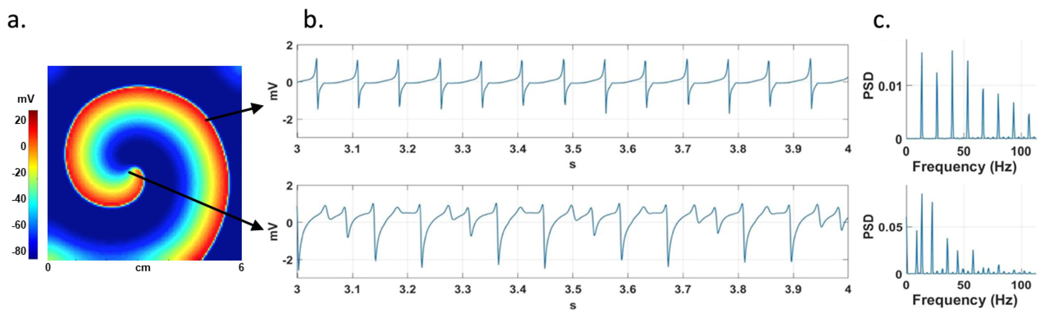
Figure 2.
Joint Directors of Laboratories (JDL) fusion model. HCI: Human computer interaction.
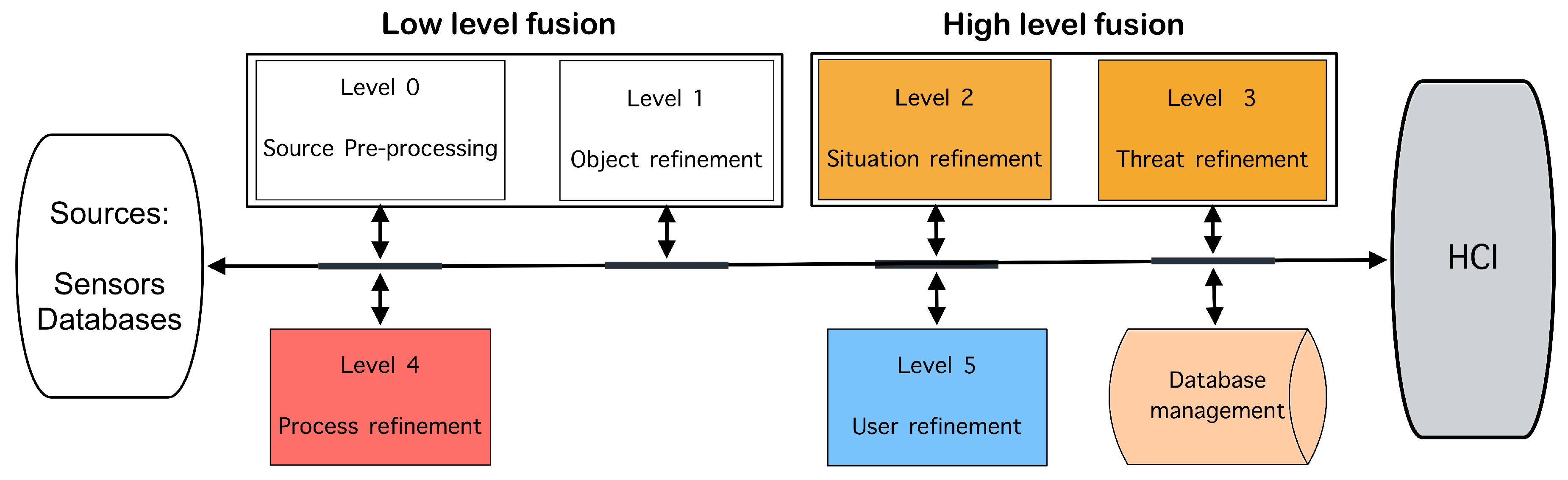
Figure 3.
Maps of the statistical features computed from the 22,500 noise-free EGMs, correspond to a rotor simulation in the 2D atrial model. a) SampEn, b) ApEn, c) Mean, d) STD, and e) ShEn. The color scale depicts the normalized values of statistics estimations.
Figure 3.
Maps of the statistical features computed from the 22,500 noise-free EGMs, correspond to a rotor simulation in the 2D atrial model. a) SampEn, b) ApEn, c) Mean, d) STD, and e) ShEn. The color scale depicts the normalized values of statistics estimations.
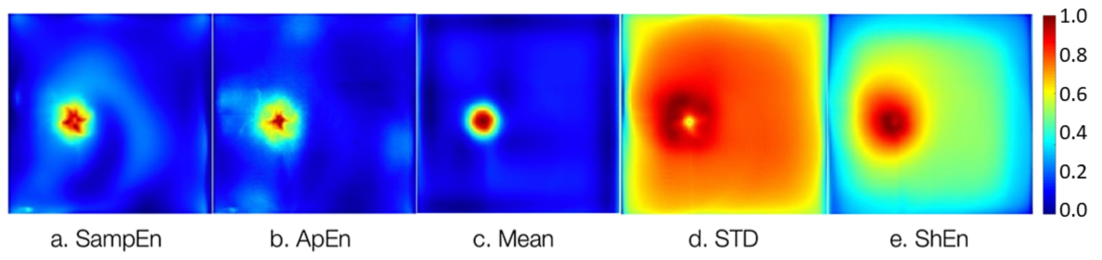
Figure 4.
Proposed JDL-based framework adapted to determine the ablation zone (rotor tip) using EGMs. The six levels of the JDL model are specified. HCI stands for human computer interaction.
Figure 4.
Proposed JDL-based framework adapted to determine the ablation zone (rotor tip) using EGMs. The six levels of the JDL model are specified. HCI stands for human computer interaction.
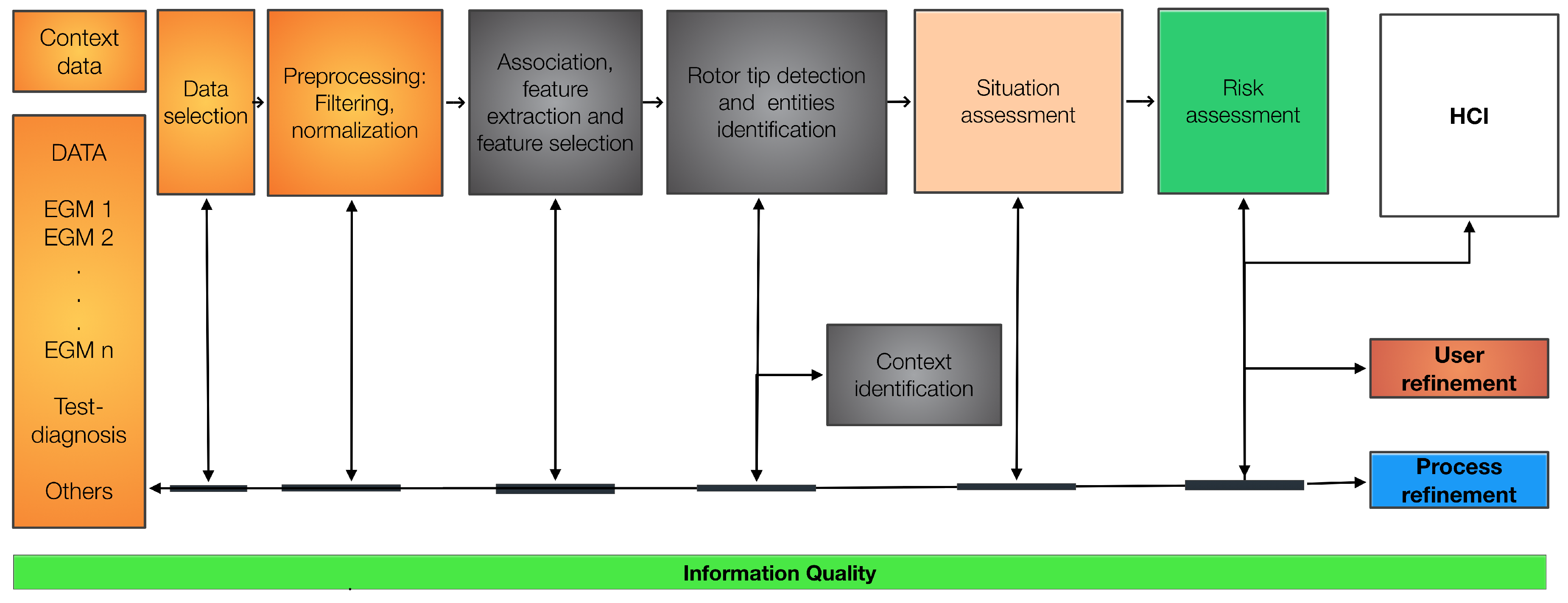
Figure 5.
Optimization process using the IQ models.
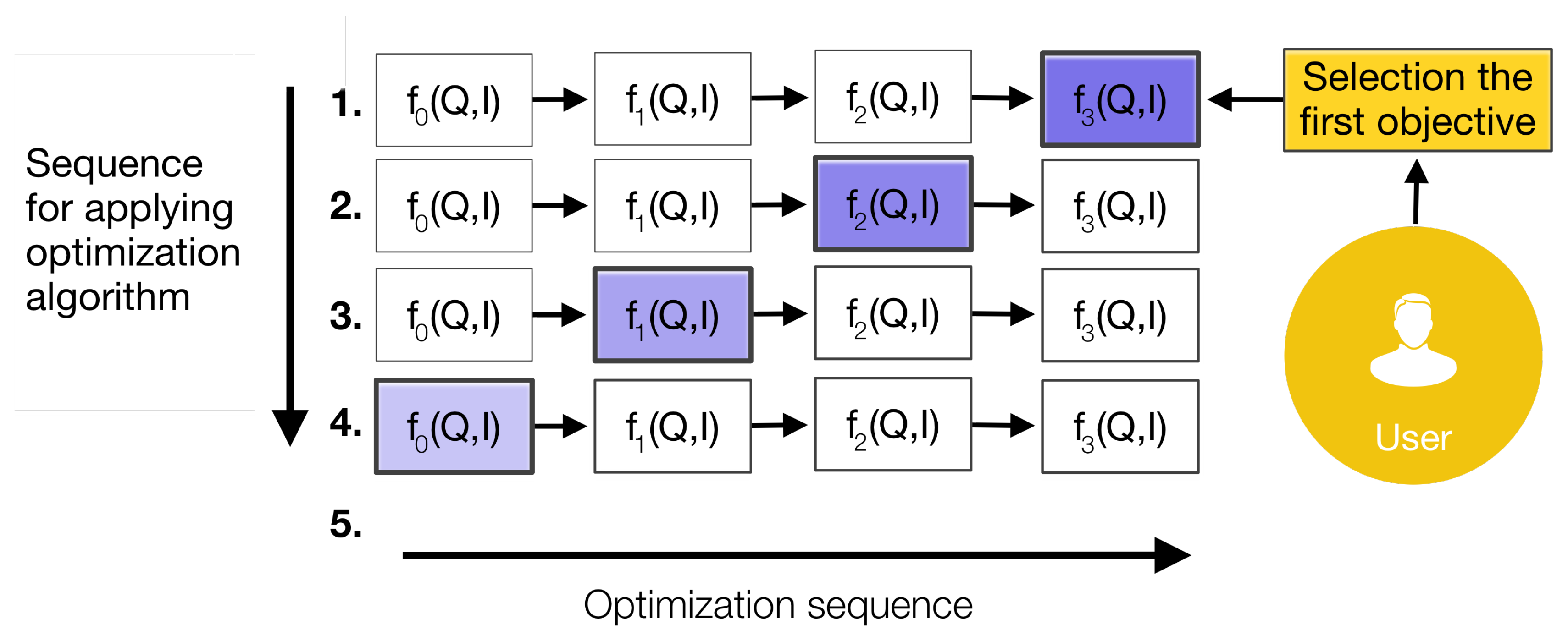
Figure 6.
Reputation and interpretability examples. a) Noise–free maps of ApEn, with a loss of 10%, and the difference between them (top). Cumulative curves for our measurements versus different values of lost samples for different maps are shown at the bottom, with the ShEn curve displayed on the left. The values of statistics estimations are not normalized. b) ApEn map and the extraction of rotor tip (top), and their interpretability (bottom) calculated based on histogram (). The red color line corresponds to data fit to a Normal distribution. The color scale depicts the normalized values of statistics estimations.
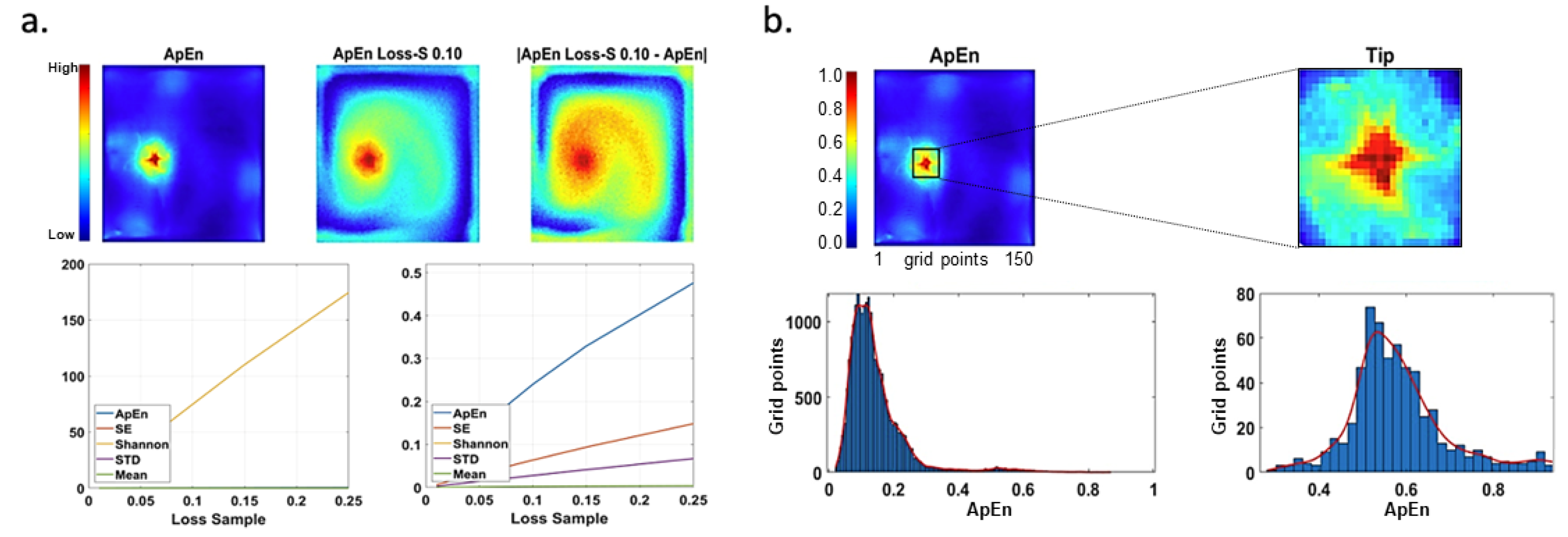
Figure 7.
Experimental procedure before testing the proposed model: a general mapping is performed on the proposed framework; then, techniques and IQ criteria (with their metrics) are selected for each level; and then, databases to validate the proposed framework are built.
Figure 7.
Experimental procedure before testing the proposed model: a general mapping is performed on the proposed framework; then, techniques and IQ criteria (with their metrics) are selected for each level; and then, databases to validate the proposed framework are built.
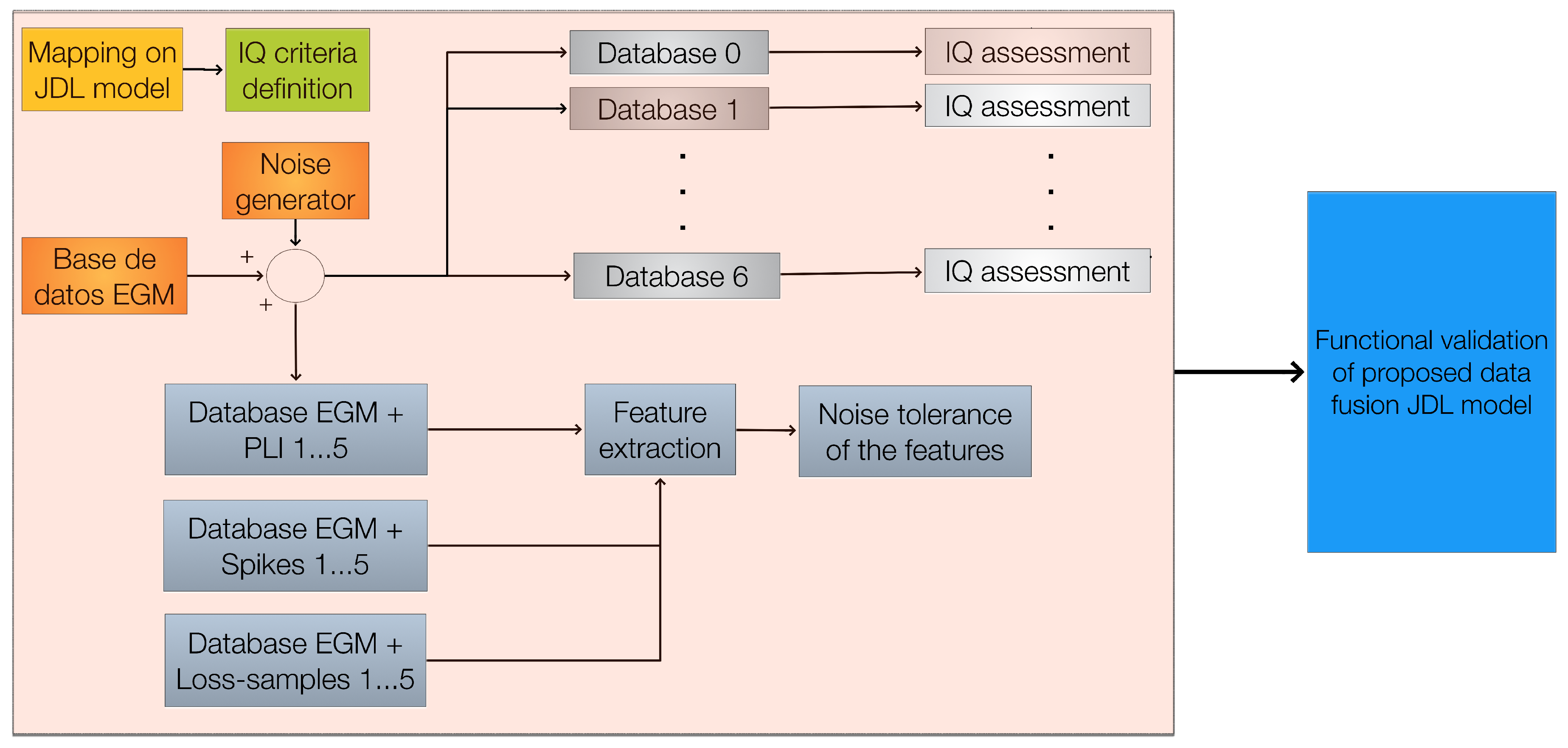
Figure 8.
Examples of different types of noise. a) One-second view of an EGM with PLI at 5 dB. b) Spikes train (red line) generated on a regular EGM (blue line) with . c) EGM with Loss Samples at 0.15. d) Loss Resolution of 0%, 75% and 97.3%, where the blank spaces indicate lost signals.
Figure 8.
Examples of different types of noise. a) One-second view of an EGM with PLI at 5 dB. b) Spikes train (red line) generated on a regular EGM (blue line) with . c) EGM with Loss Samples at 0.15. d) Loss Resolution of 0%, 75% and 97.3%, where the blank spaces indicate lost signals.
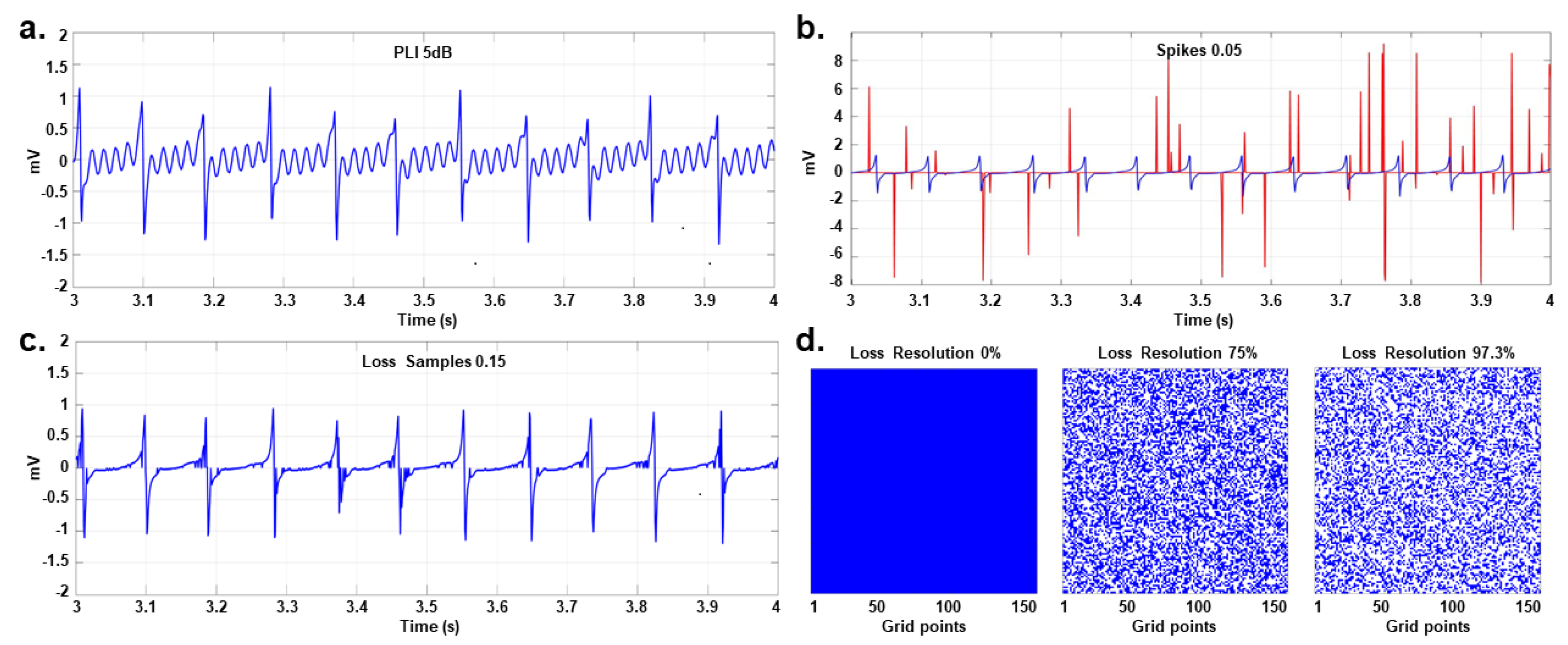
Figure 9.
Statistical feature maps affected by different levels of perturbations. a) Loss Samples. b) Spikes, and c) PLI. The color scale depicts the normalized values of statistics estimations.
Figure 9.
Statistical feature maps affected by different levels of perturbations. a) Loss Samples. b) Spikes, and c) PLI. The color scale depicts the normalized values of statistics estimations.
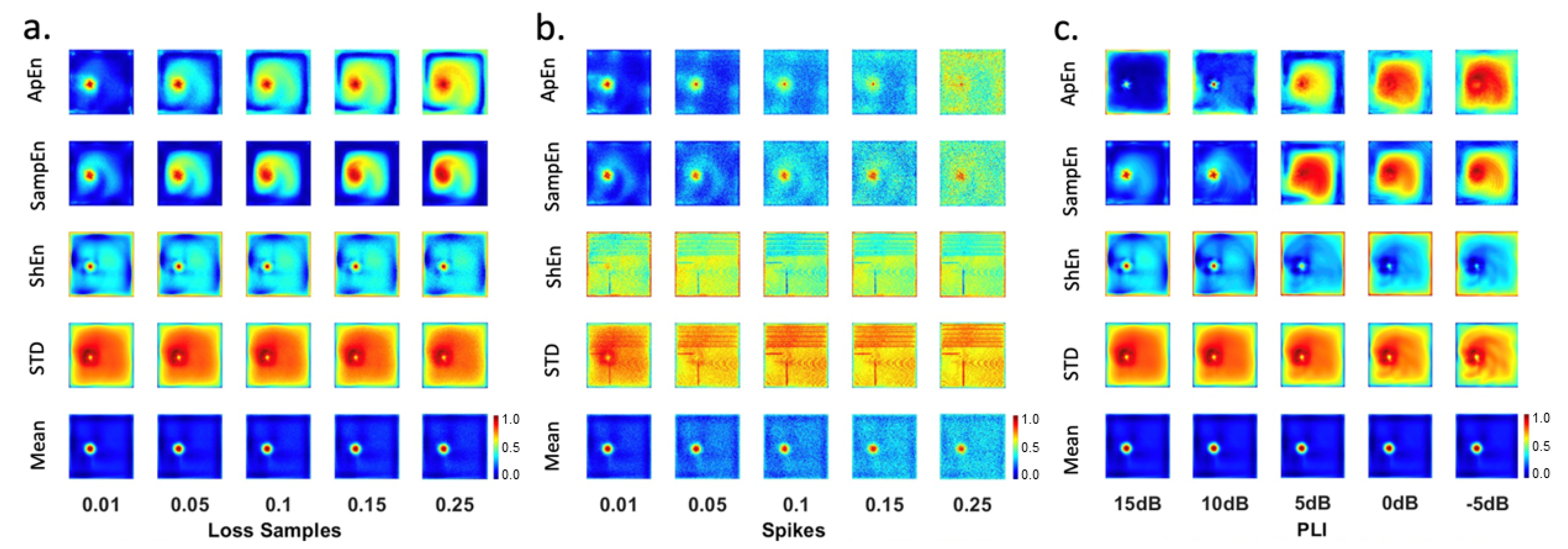
Figure 10.
Statistical feature maps affected by different levels of perturbations of loss samples/spikes/PLI with a) loss resolution of 0%, and b) loss resolution of 97.3%. The color scale depicts the normalized values of statistics estimations.
Figure 10.
Statistical feature maps affected by different levels of perturbations of loss samples/spikes/PLI with a) loss resolution of 0%, and b) loss resolution of 97.3%. The color scale depicts the normalized values of statistics estimations.
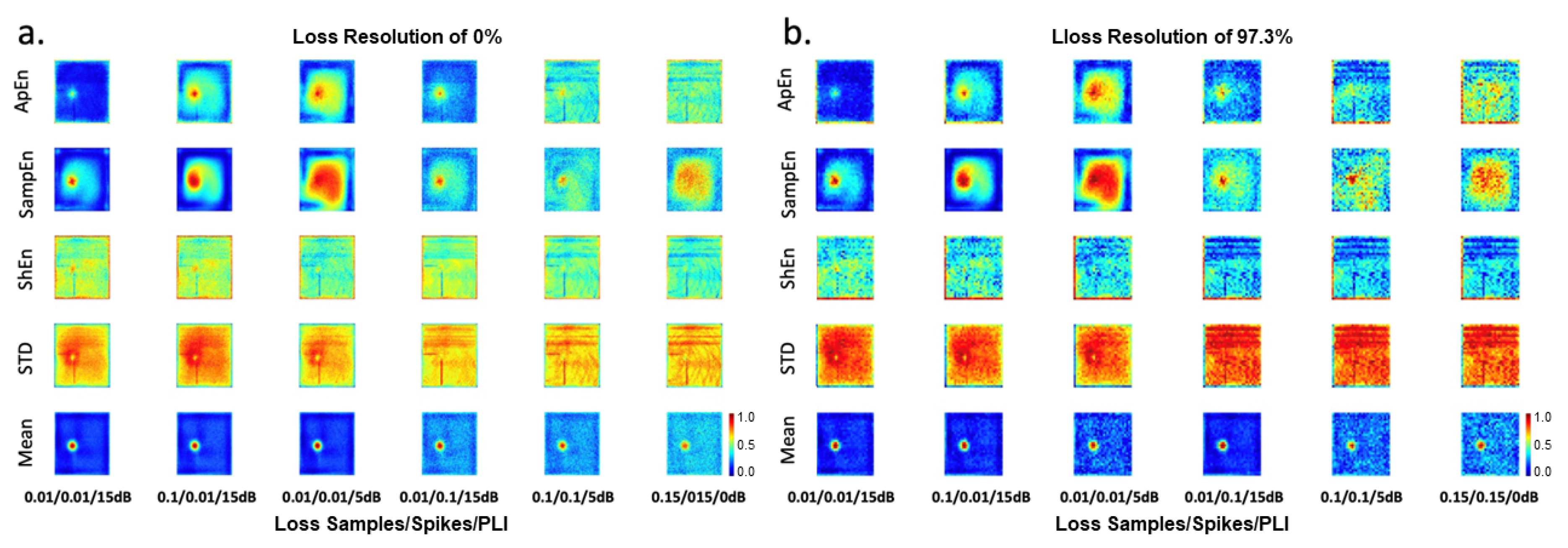

Table 1.
Definitions of information quality criteria and metrics by level.
| Level | Criteria | Metric | Equation |
|---|---|---|---|
| 0 | Accuracy | Number of spikes (), power relation between component of 60Hz and the total power of the signal. |
, where m is the number of the signals. , where is the power of the component of 60Hz, and is the total power of all EGM signals. |
| 0 | Precision | Sample rate (Ts) | |
| 0 | Data amount | Resolution (Res) | where, is the number of virtual electrodes by row and is the number of virtual electrodes by column. |
| 0 | Completeness | Number of lost samples per signal (); Number of lost signals () |
, where m is the number of signals and is the number of samples for each signal. is the number the elements of its argument set, P holds the power values of a total of N signals. denotes zero-power signals and denotes non-zero-power signals. |
| 1 | Relevancy | Relevance of features () | ; ; w: weights for each feature. |
| 1 | Consistency | Distance among measures (e.g. SampEn, ApEn) |
, for the i–th and j–th features of the map. |
| 1 | Accuracy | Difference between ground truth and detected rotor tip |
, where is the calculated and is the ground truth. |
| 1 | Precision | Deviation of distances among features (5%) nearest to tip |
, where n is the 5% of the features nearest to rotor tip. |
| 1, 2 | Reputation | Noise tolerance of the features. This quantifies the noise tolerance | |
| 2 | Interpretability | Quality of the map figure for showing the rotor tip location based on the contrast | , where is the mean measure and is the bandwidth of the distribution of the data of the map and and (5% of high values) are the mean and bandwidth of the distribution of the Tip. |
| 2, 3 | Objectivity | It is the objective assessment given by the quality of the information | , where is the Global IQ evaluate until level 2 or 3 depends of level and is the IQ of level n. |
| 3 | Accuracy | Accuracy with respect to the prediction made by the expert supported by the system | , where is the number of successful predicted events and is the total events. |
| 0-5 | Efficiency | Computational cost | , where is processing time given in seconds. |
| 5 | Authority | Experience and effectiveness of the doctor for conducing treatments. | It is assigned by the expert from the interval . |
Table 2.
Configuration of EGM perturbations for each validation database.
| Database | Loss Samples | Spikes | PLI | Loss Resolution |
|---|---|---|---|---|
| 1 | 0.01 | 0.01 | -5 dB | 0% |
| 2 | 0.05 | 0.05 | 0 dB | 75% |
| 3 | 0.10 | 0.1 | 5 dB | 93.5% |
| 4 | 0.15 | 0.15 | 10 dB | 97.3% |
| 5 | 0.25 | 0.25 | 0.15 dB | 99% |
Table 3.
Correlation between pairs of quality criteria from level 0.
| Database | Accuracy–spikess | Accuracy–PLII | Data–amount | Completeness | Loss Sample | PLI | Spikes |
|---|---|---|---|---|---|---|---|
| Accuracy–spikes | 1 | 0.009 | 0.001 | 0.317 | 0.097 | 0.199 | 0.977 |
| Accuracy–PLI | 0.009 | 1 | 0.994 | 0.001 | 0.007 | 0.008 | 0.010 |
| Data–amount | 0.001 | 0.994 | 1 | 0.001 | 1.146e-17 | 2.502e-18 | 3.102e-17 |
| Completeness | 0.317 | 0.001 0.001 | 1 | 0.804 | 0.265 | 0.280 | |
| Loss–Sample | 0.097 | 0.007 | 1.146e-17 | 0.804 | 1 | 0.139 | 0.075 |
| PLI | 0.199 | 0.008 | 2.502e-18 | 0.265 | 0.139 | 1 | 0.139 |
| Spikes | 0.977 | 0.010 | 3.102e-17 | 0.280 | 0.075 | 0.139 | 1 |
Table 4.
Correlation between pairs of IQ criteria from level 1.
| Noise | Consistency | Precision | Reputation | Accuracy |
|---|---|---|---|---|
| Consistency | 1 | 0.293 | 0.187 | 0.427 |
| Precision | 0.293 | 1 | 0.286 | 0.552 |
| Reputation | 0.187 | 0.286 | 1 | 0.487 |
| Accuracy | 0.427 | 0.552 | 0.487 | 1 |
Table 5.
Correlation between pairs of IQ criteria of level 1 (input-output).
| IQ of Level 1 outputs | IQ of Level 1 inputs | ||||||||||
|---|---|---|---|---|---|---|---|---|---|---|---|
| Criteria | Consistency | Precision | Reputation | Accuracy | Acc–Spikes | Acc–PLI | D–amount | Compl. | LSamp | PLI | Spikes |
| Consistency | 1.00 | 0.38 | 0.15 | 0.02 | 0.36 | 0.29 | 0.30 | 0.65 | 0.45 | 0.28 | 0.33 |
| Precision | 0.38 | 1.00 | 0.23 | 0.01 | 0.30 | 0.49 | 0.50 | 0.21 | 0.08 | 0.10 | 0.31 |
| Reputation | 0.15 | 0.23 | 1.00 | 0.00 | 0.37 | 0.00 | 0.00 | 0.11 | 0.01 | 0.07 | 0.37 |
| Accuracy | 0.02 | 0.01 | 0.00 | 1.00 | 0.10 | 0.03 | 0.03 | 0.03 | 0.09 | 0.03 | 0.09 |
Table 6.
Correlation between pairs of IQ criteria of level 2 (input-output).
| IQ of Level 2 outputs | IQ of Level 2 inputs | |||||||
|---|---|---|---|---|---|---|---|---|
| Criteria | Interp. | Rep. | Object. | Effic. | Cons. | Prec. | Rep. | Acc. |
| Interpretability | 1.00 | 0.11 | 0,39 | 0.45 | 0.22 | 0.36 | 0,45 | 0.28 |
| Reputation | 1.00 | 0.32 | 0.02 | 0.19 | 0.15 | 0.68 | 0.45 | |
| Objectivity | 1.00 | 0.00 | 0.45 | 0.22 | 0.15 | 0.33 | ||
| Efficiency | 1.00 | 0.01 | 0.00 | 0.00 | 0.01 | |||
Table 7.
Correlation between pairs of IQ criteria of level 3 (input-output).
| IQ of Level 3 outputs | IQ of Level 3 inputs | ||||||
|---|---|---|---|---|---|---|---|
| Criteria | Acc. | Object. | Effic. | Interp. | Rep. | Object. | Effic. |
| Accuracy | 1.00 | 0.41 | 0.02 | 0.56 | 0.24 | 0.32 | 0.00 |
| Objectivity | 1.00 | 0.00 | 0.41 | 0.12 | 0.63 | -0.01 | |
| Efficiency | 1.00 | 0.00 | 0.00 | 0.03 | 0.01 | ||
Table 8.
Performance (error) of SVR models of IQ of level 1.
| Measures | Consistency | Precision | Reputation | Accuracy |
|---|---|---|---|---|
| MAE | 0.0634 | 0.1682 | 0.0289 | 0.0033 |
| RMSE | 0.1198 | 0.2185 | 0.1123 | 0.0046 |
| MAPE | 0.6891 | 2.5689 | 1.5013 | 0.0981 |
Table 9.
Performance (error) of SVR models of IQ of level 2.
| Measures | Consistency | Precision | Reputation | Accuracy |
|---|---|---|---|---|
| MAE | 0.0634 | 0.1682 | 0.0289 | 0.0033 |
| RMSE | 0.1198 | 0.2185 | 0.1123 | 0.0046 |
| MAPE | 0.6891 | 2.5689 | 1.5013 | 0.0981 |
Table 10.
Performance (error) of SVR models of IQ of level 3.
| Measures | Consistency | Precision | Reputation | Accuracy |
|---|---|---|---|---|
| MAE | 0.0634 | 0.1682 | 0.0289 | 0.0033 |
| RMSE | 0.1198 | 0.2185 | 0.1123 | 0.0046 |
| MAPE | 0.6891 | 2.5689 | 1.5013 | 0.0981 |
Disclaimer/Publisher’s Note: The statements, opinions and data contained in all publications are solely those of the individual author(s) and contributor(s) and not of MDPI and/or the editor(s). MDPI and/or the editor(s) disclaim responsibility for any injury to people or property resulting from any ideas, methods, instructions or products referred to in the content. |
© 2024 by the authors. Licensee MDPI, Basel, Switzerland. This article is an open access article distributed under the terms and conditions of the Creative Commons Attribution (CC BY) license (http://creativecommons.org/licenses/by/4.0/).
Copyright: This open access article is published under a Creative Commons CC BY 4.0 license, which permit the free download, distribution, and reuse, provided that the author and preprint are cited in any reuse.


