On the Extended Simple Equations Method (SEsM) and its Application to the Time--Fractional Diffusive Predator--Prey System Incorporating an Allee Effect

1. Introduction

In the recent two decades, the use of time– and space– fractional nonlinear partial differential equations (FNPDEs) has become increasingly popular in the scientific society to model and study various natural processes. This approach allows for capturing the complexities inherent in many real-world systems occurring in in the fields of biology and ecology [1,2,3], fluid mechanics [4,5,6,7], finance and economics [8,9,10], engineering [11,12,13], etc. The main features of such real-word systems are they are characterized by memory effects, spatial heterogeneity and non-local interactions, which traditional integer–order models cannot account for. One direction to elucidate these non–specific dynamical effects is to derive and analyze analytical solutions of the fractional models. Finding analytical solutions of FNPDEs, however, is a challenging task due to the complexity introduced by both the nonlinearity and the fractional order of the derivatives.

Recently, two basic approaches for extracting exact solutions of FNPDEs are used: 1) Applying fractional transformation which allows to reduce the studied NFPDEs to integer–order nonlinear ODEs, and then using well–established techniques from the theory of integer-order NPDEs to obtain exact general and particular solutions of NPDEs. For this scenario, there are many general methodologies, including use of ansatz techniques [14,15,16,17,18,19], group analysis [20,21], perturbation methods [22,23], decomposition methods [27,28] and so on; 2) Applying standard traveling wave transformation which allows to reduce the studied NFPDEs to simpler fractional differential equations (in most cases, to fractional ODEs) and using their known solutions in constructing the solutions of the basic NPDEs[29]. In this category, the most popular method is so called fractional sub–equation method [24], which uses known solution of the fractional version of an ODE of Riccati in deriving analytical solutions of the studied FPDEs. Later, improvements of the fractional sub-equation method are made in [25,26].

The generalized methodology proposed in this article includes both approaches mentioned above, allowing the researcher to choose which of the two techniques to apply. In detail, as it will be shown in the next section of this paper,firstly we extend the SEsM [30,31,32], which is established for finding exact solutions of integer–order NPDEs and then we adapt it to finding exact solutions of systems of FNPDEs by introducing of appropriate traveling wave transformations. Unlike other analytical methods in this scientific field, SEsM give opportunity to present the solutions of studied NPDEs as compositions, including series of solutions of more than one simple equation or more than one special function. The new and different emphasis in the extended version of the SEsM is assumption that the simple equations used have different variables. This new approach based on the SEsM, has been first applied to find analytical solutions of the extended integer–order KDV equation in [33]. Later, in [34], the authors proposed independently a similar methodology based on the Extended Kudryashov Method, as it was applied to find exact solutions of the integer–order Bossinesq–like system. In constructing solutions of this system, however, the authors used only versions of ODEs of Riccati as simple equations. In terms of finding exact solutions of FNPDEs, in [43,44], the SEsM was applied to obtain numerous exact solutions of systems of FNPDEs, modeling natural processes in fluid mechanics and ecology. The obtained analytical solutions included two simple equations with one independent variable. Various types of simple equations were used, including first-order ODEs, like ODE of Riccati, ODE of Bernoulli and ODE of Abel of first kind, as well as second-order ODEs involving various hyperbolic and elliptic functions. As it was shown in [43,44], depending on the type of simple equations selected, the obtained analytical solutions recreate in more accurate way the complex wave behavior of the modeled real–word processes, which includes multi–soliton interactions, breather states and other multi-wave phenomena. In the above-mentioned articles, the studied FNPDEs were reduced to integer-order ODEs using a fractional transformation. However, a different approach to selecting a traveling wave transformation also exists and it will be presented in the next section of this article.

The publication is structured as follows: In Section 2, we present the generalized SEsM algorithm for finding exact solutions of systems of FNPDEs (in particular, for single FNPDEs). In Section 3 and Section 4, we apply several variants of the generalized SEsM algorithm, proposed in Section 2, to derive exact solutions of the time-fractional predator-prey system under the Allee effect. According to the generalized SEsM algorithm, we consider two cases related to the choice of traveling wave transformation used for obtaining analytical solutions of the studied system: Variant 1 (In section 3): Use of a fractional transformation that reduces the studied system of FNPDEs to a system of integer-order ODEs and using simple integer-order ODEs with known analytical solutions as simple equations; Varant 2 (In Section 4): Use of a standard traveling wave transformation that reduces the studied system of FNPDEs to a system of fractional ODEs and using simple fractional ODEs with known analytical solutions as simple equations. In Section 5, numerical illustrations of some of the obtained analytical solutions are provided, along with a brief explanation of the numerical results obtained. Section 6 contains concluding remarks summarizing the basic findings of the study.

2. Description of the Generalized SEsM Algorithm and Statement of the Studied Problem

In this section we shall present the extended SEsM algorithm in detail, exposing all the possibilities it offers for finding diverse types of complex analytical solutions of systems FNPDEs (in particular, systems of nonlinear PDEs (NPDEs), as well as single FNPDEs and single NPDEs ). As it will be shown below, in contrast to the original SEsM algorithm presented in [30,31,32], we exchange its first and second steps, as extensions in the methodology are made to both steps of the original SEsM algorithm.

Now we shall focus on the simplest case of a system of two NFPDEs with two independent variables:

$$\begin{array}{ccc}& & \Psi (u(x,t),D_t^{\alpha }u(x,t),D_x^{\beta }u(x,t),D_{tt}^{2\alpha }u(x,t),D_{xx}^{2\beta }u(x,t),...)=0\hfill \\ & & \Omega (v(x,t),D_t^{\alpha }v(x,t),D_x^{\beta }v(x,t),D_{tt}^{2\alpha }v(x,t),D_{xx}^{2\beta }v(x,t),...)=0,0<\alpha ,\beta \le 1\hfill \end{array}$$

(1)

where D denotes the arbitrary fractional order derivative operator, as superscripts $\alpha ,\beta ,2\alpha ,2\beta ..$ give its fractional number and subscripts denote time and partial derivatives. Here, $\Psi$ and $\Omega$ are polynomials of $u(t,x)$ and $v(t,x)$ and its derivatives, respectively, where $u=u(t,x)$ and $v=v(t,x)$ are unknown functions.

Firstly, to be able to apply the SEsM to Eqs (1), it is very important to define the fractional derivatives presented in Eqs (1). Defining the type of fractional derivatives in FNPDEs which model wave dynamics of real–world processes is essential for accurately reflecting the system’s physical properties. The choice between fractional derivatives like Riemann-Liouville, Caputo or conformable derivatives depends on factors such as the nature of the process, boundary conditions, and the desired interpretation of memory effects.

The generalized extended SEsM algorithm which is adopted for extracting exact analytical solutions of FNPDEs involves the following basic steps:

• Construction of the solutions of Eqs (1). Apart from the traditional construction of solutions of Eqs (1), which involve the solution of one simple (auxiliary) equation with one independent variable (e.g. [35,36,37,38,39]), the SEsM also offers the following possible variants for constructing these solutions:
  • Variant 1: The solutions of Eqs (1) can be presented by single composite functions with different independent variables for each system variable (This solution variant is applicable to real–world dynamical models of a type (1), where it is expected that the system variables move with different wave speeds):

    $$u\left({\xi }_1\right)=F_1\left({\xi }_1\right),v\left({\xi }_2\right)=F_2\left({\xi }_2\right),$$

    (2)

    where

    $$F_1\left({\xi }_1\right)=\sum _{i_1=1}^{n_1}{a}_{i_1}{\left[f_1\left({\xi }_1\right)\right]}^{i_1},F_2\left({\xi }_2\right)=\sum _{i_2=1}^{n_2}{b}_{i_2}{\left[f_2\left({\xi }_2\right)\right]}^{i_2},$$

    (3)

    as $f_1\left({\xi }_1\right)$ and $f_2\left({\xi }_2\right)$ are the solutions of simple equations, presented in the following general form:

    $${\left({\displaystyle \frac{d^{k_1}{f}_1}{d{\xi }_1^{k_1}}}\right)}^{l_1}=\sum _{j_1=0}^{m_1}{c}_{j_1}{f}_1^{j_1},{\left({\displaystyle \frac{d^{k_2}{f}_2}{d{\xi }_2^{k_2}}}\right)}^{l_2}=\sum _{j_2=0}^{m_2}{d}_{j_2}{f}_2^{j_2},$$

    (4)

    where $k_{1,2}$ are the orders of derivatives of $f_1$ and $f_2$, $l_{1,2}$ are the degrees of derivatives in the defining ODEs and $m_{1,2}$ are the highest degrees of the polynomials of $f_1$ and $f_2$ in the defining ODEs.
  • Variant 2: The solutions of Eqs (1) can be presented as complex composite functions of two or more single composite functions, involving solutions of two or more simple equations, which have different independent variables for each system variable (This solution variant is applicable to real–world dynamical models of a type (1) with complex multi–wave dynamics, where it is expected that the system variables move with different wave speeds). The simplest example of a such solution is:

    $$u\left({\xi }_1\right)=F_1\left({\xi }_1\right)+F_2\left({\xi }_1\right),v\left({\xi }_2\right)=F_3\left({\xi }_2\right)+F_4\left({\xi }_2\right),$$

    (5)

    where

    $$\begin{array}{c}\hfill F_1\left({\xi }_1\right)=\sum _{i_1=1}^{n_1}{a}_{i_1}{\left[f_1\left({\xi }_1\right)\right]}^{i_1},F_2\left({\xi }_1\right)=\sum _{i_2=1}^{n_2}{b}_{i_2}{\left[f_2\left({\xi }_1\right)\right]}^{i_2},\\ \hfill F_3\left({\xi }_2\right)=\sum _{i_3=1}^{n_3}{g}_{i_3}{\left[f_3\left({\xi }_2\right)\right]}^{i_3},F_4\left({\xi }_2\right)=\sum _{i_4=1}^{n_4}{h}_{i_4}{\left[f_4\left({\xi }_2\right)\right]}^{i_4},\end{array}$$

    (6)

    as $f_1\left({\xi }_1\right),f_2\left({\xi }_1\right)$ and $f_3\left({\xi }_2\right),f_4\left({\xi }_2\right)$ are solutions of simple equations of kind (4).
    Note: This variant of the solution is very difficult to derive due to difficulties in the analytical calculations of the coefficients $a_{i_1},b_{i_2},g_{i_3},h_{i_4}$ in Eqs (6). One option to obtain solutions of this kind is to use simple equations of type (4) with a almost uniform structure and simpler polynomial parts.
  • Variant 3: The solutions of Eqs (1) can be presented as complex composite functions of two or more single composite functions, involving solutions of two or more simple equations, with one independent variable for both system variable (This solution variant is applicable to real–world dynamical models of a type (1), where it is expected that the system variables move at uniform wave speed, but they exhibit synchronized multi–wave behavior). The simplest example of a such solution is:

    $$u\left(\xi \right)=F_1\left(\xi \right)+F_2\left(\xi \right),v\left(\xi \right)=F_3\left(\xi \right)+F_4\left(\xi \right),$$

    (7)

    where

    $$\begin{array}{c}\hfill F_1\left(\xi \right)=\sum _{i_1=1}^{n_1}{a}_{i_1}{\left[f_1\left(\xi \right)\right]}^{i_1},F_2\left(\xi \right)=\sum _{i_2=1}^{n_2}{b}_{i_2}{\left[f_2\left(\xi \right)\right]}^{i_2},\\ \hfill F_3\left(\xi \right)=\sum _{i_3=1}^{n_3}{g}_{i_3}{\left[f_1\left(\xi \right)\right]}^{i_3},F_4\left(\xi \right)=\sum _{i_4=1}^{n_4}{h}_{i_4}{\left[f_2\left(\xi \right)\right]}^{i_4},\end{array}$$

    (8)

    as $f_1\left(\xi \right)$ and $f_2\left(\xi \right)$ are solutions of simple equations of kind (4).
  • Variant 4: The solutions of Eqs (1) can be presented as complex composite functions of two or more single composite functions, involving solutions of two or more simple equations with different independent variables. (This solution variant can be realized only for real–world dynamical models of a type (1), where it is expected that the system variables move at uniform wave speed, but they exhibit complex synchronized multi–wave behavior). The simplest example of a such solution is:

    $$u({\xi }_1,{\xi }_2)=F_1\left({\xi }_1\right)+F_2\left({\xi }_2\right),v({\xi }_1,{\xi }_2)=F_3\left({\xi }_1\right)+F_4\left({\xi }_2\right),$$

    (9)

    where

    $$\begin{array}{c}\hfill F_1\left({\xi }_1\right)=\sum _{i_1=1}^{n_1}{a}_{i_1}{\left[f_1\left({\xi }_1\right)\right]}^{i_1},F_2\left(\xi \right)=\sum _{i_2=1}^{n_2}{b}_{i_2}{\left[f_2\left({\xi }_2\right)\right]}^{i_2},\\ \hfill F_3\left(\xi \right)=\sum _{i_3=1}^{n_3}{g}_{i_3}{\left[f_1\left({\xi }_1\right)\right]}^{i_3},F_4\left(\xi \right)=\sum _{i_4=1}^{n_4}{h}_{i_4}{\left[f_2\left({\xi }_2\right)\right]}^{i_4},\end{array}$$

    (10)

    as $f_1\left({\xi }_1\right)$ and $f_2\left({\xi }_2\right)$ are solutions of the simple equations (4).
  Note: Other expressions of the solutions of Eq. (1) which involve product or division of single composite functions in the corresponding complex composite functions are also possible.
• Selection of the traveling wave type transformation.
  • Variant 1: Use a fractional transformation. The choice of explicit form of the fractional traveling wave transformation depends on how the fractional derivatives in Eq. (1) are defined at the beginning. Bellow, the most used fractional traveling wave transformations are selected:
    – Conformable fractional traveling wave transformation: ${\xi }_1={\kappa }_1{\displaystyle \frac{x^{\beta }}{\beta }}+{\omega }_1{\displaystyle \frac{t^{\alpha }}{\alpha }},{\xi }_2={\kappa }_2{\displaystyle \frac{x^{\beta }}{\beta }}+{\omega }_2{\displaystyle \frac{t^{\alpha }}{\alpha }},..$, defined for conformable fractional derivatives [34];
    – Fractional complex transform: ${\xi }_1={\kappa }_1{\displaystyle \frac{x^{\beta }}{\Gamma (\beta +1)}}+{\omega }_1{\displaystyle \frac{t^{\alpha }}{\Gamma (\alpha +1)}},{\xi }_2={\kappa }_2{\displaystyle \frac{x^{\beta }}{\Gamma (\beta +1)}}+{\omega }_2{\displaystyle \frac{t^{\alpha }}{\Gamma (\alpha +1)}}..$, defined for modified Riemann–Liouville fractional derivatives [41], which can applied for for Caputo fractional derivatives and other fractional deriatis in studing FNPDEs [46].
    In the both cases, the studied FNPDEs are reduced to integer–order nonlinear ODEs.
  • Variant 2: Use a standard traveling wave transformation. In this case, introduction of traveling wave ansatz ${\xi }_1={\kappa }_{1}x+{\omega }_{1}t,{\xi }_2={\kappa }_{2}x+{\omega }_{2}t,..$ in Eqs (1) reduces the studied FNPDEs to fractional nonlinear ODEs. In accordance with the method used in this case (see Ref. [24,25,26]), however, Eqs (1) must be defined by Jumarie’s modified Riemann-Liouville derivatives [41].
• Selection of the forms of the used simple equations.
  • For Variant 1 of Step 2: By fixation of $k_1,k_2$,$l_1,l_2$ and $m_1,m_2$ in Eqs (4), different types integer–order ODEs can be used as simple equations, such as:
    – ODEs of first order (an ODE of Riccati, an ODE of Bernoulli, an ODE of Abel of first kind, an ODE of tanh–function,etc);
    – ODEs of second order (elliptic functions of Jaccobi and Weiershtrass, an ODE of Abel of second kind, etc.) (when is possible)
  • For Variant 2 of Step 2: The fractional version of an ODE of Riccati and its sub–variants (depending on numerical values of its coefficients) only can be used as simple equations.
  Note: The correct choice of simple equations used depends on the type of waves that are realistic for the physical process being modeled by the corresponding FNPDES. This is because different ODEs correspond to different wave dynamics, such as shock waves, solitons, or oscillatory patterns, and selecting the right equation is essential for accurately describing the system’s behavior.
• Derivation of the balance equations and the system of algebraic equations. The fixation of the explicit form of constructed variant solutions of Eqs (1) presented in Step 1 of the SEsM algorithm depends on the balance equations derived. As a result, a polynomial of the functions $f_1$ and $f_2$ (for Variant 1 and Variants 3-4 in Step 1) or a polynomial of the functions $f1,f_2,f_3,f_4$ (for Variant 2 in Step 1) is obtained. The coefficients in front of these functions include the coefficients of the solution of the considered FNPDEs as well as the coefficients of the simple equations used. Analytical solutions of Eqs (1) can be extracted only if each coefficient in front of the functions $f_1$ and $f_2$ (or the functions $f1,f_2,f_3,f_4$ ) contains almost two terms. Equating these coefficients to zero leads to formation of a system of nonlinear algebraic equations for each variant chosen according Steps 1,2 and 3 of the SEsM algorithm.
• Derivation of the analytical solutions. Any non–trivial solution of the algebraic system above mentioned leads to a solution of the studied FNPDEs by replacing the specific coefficients in the corresponding variant solutions, given in Step 1 as well as by changing the traveling wave coordinates chosen by the variants given in Step 2.

Note: The methodology above given can also be applied for finding exact analytical solutions of single FNPDEs, as their solution forms are similar to those presented in Variant 3 and Variant 4 from Step 1 of the SEsM algorithm. Additionally, the generalized SEsM algorithm presented above can be applied for obtaining analytical solutions of standard NPDEs by using a standard traveling wave transformation in Step 2 from the algorithm.

The general algorithm outlined above aims to assist researchers in this field in finding analytical solutions for models of type (1) describing natural processes. Based on it, they can make their choice between the variants given in steps 1,2 and 3, taking into account the specific features of the wave dynamics of the modeled natural phenomenon.

In this paper, we shall consider the time-fractional re–scaled version of the diffusive predator–prey model proposed in [45]:

$$\begin{array}{c}\hfill D_t^{\varphi }u=u_{xx}-\beta u+(\beta +1)u^2-u^3-(1+\alpha v)uv,\\ \hfill \kappa D_t^{\varphi }v=v_{xx}+\sigma (1+\alpha v)uv-{\mu }_{1}v-{\mu }_2{v}^2-{\mu }_3{v}^3\end{array}$$

(11)

where $u(x,t)$ and $v(x,t)$ are re–scaled sizes or densities of the prey and predator populations, respectively, $\varphi$ is the time–fractional derivative order, and $\alpha ,\beta ,\sigma ,{\mu }_1,{\mu }_2,{\mu }_3$ are constants. Eqs (11) describe the complex dynamical behaviour of the predator and the prey populations which are both subject to the Allee effect. A detailed description for modeling this double effect is in the predator–prey system given in [45]. Similar to the research carried out in [45], we shall search for analytical solutions of the system (11) assuming that the population waves of the predator and the prey propagate at different speeds. Then, for the simplest case, the general solution of Eqs (11) can be presented by two single composite functions with different independent variables for each variable of Eqs (11) (Variant 1 of Step 1 of the SEsM algorithm). We shall search for analytical solutions of Eqs (11) in two different ways: 1) By introducing fractional traveling wave transformation and using the specter of available integer–order ODEs with known solutions (in Section3); 2) By introducing standard traveling wave transformation and using one version of the fractional ODE of Riccati with known solutions (in Section 4). Regarding to Case 1, some of the key ideas related to the current study were outlined in [45], which we further develop and expand upon here.

3. Exact Solutions of the Time–Fractional Diffusive Predator–Prey System Incorporating an Allee Effect Using Fractional Transformation.

We present the general solution of Eqs (11) as follows:

$$\begin{array}{c}\hfill u\left({\xi }_1\right)=F_1\left({\xi }_1\right)=\sum _{i_1=1}^{n_1}{a}_{i_1}{\left[f_1\left({\xi }_1\right)\right]}^{i_1},\\ \hfill v\left({\xi }_2\right)=F_2\left({\xi }_2\right)=\sum _{i_2=1}^{n_2}{b}_{i_2}{\left[f_2\left({\xi }_2\right)\right]}^{i_2},\end{array}$$

(12)

In view of the biological nature of the studied time–fractional predator–prey model, we choose to represent the memory effects occurring in the system (11) in the sense of a Caputo derivative [46]. Thus, the fractional transformations take the form:

$${\xi }_1=x-{\displaystyle \frac{{\omega }_1{t}^{\varphi }}{\Gamma (1+\varphi )}},{\xi }_2=x-{\displaystyle \frac{{\omega }_2{t}^{\varphi }}{\Gamma (1+\varphi )}},0\le \varphi \le 1$$

(13)

We choose the simple equations used to be nonlinear ODEs of first order:

$${\displaystyle \frac{d{f}_1}{d{\xi }_1}}=\sum _{j_1=0}^{m_1}{c}_{j_1}{\left[f_1\left({\xi }_1\right)\right]}^{j_1},{\displaystyle \frac{d{f}_2}{d{\xi }_2}}=\sum _{j_2=0}^{m_2}{d}_{j_2}{\left[f_2\left({\xi }_2\right)\right]}^{j_2}$$

(14)

For simplicity, bellow we shall present these solutions by the special functions $V_{c_0,c_1,..c_{j_1}}({\xi }_1;1,1,m_1)$ and $V_{d_0,d_1,..d_{j_2}}({\xi }_2;1,1,m_2)$, which are written in the context of Eqs (14).

Due to the nature of the studied model, we assume also that the two simple equations used have an identical form. The balance equations are $n_1=m_1-1,n_2=m_2-1$. Bellow we shall present various solutions of Eqs (11) depending on the specific form of the simple equations used.

3.1. Case 1: For $m_1=3$ and $m_2=3$

3.1.1. Variant 1: For $c_0\ne 0,c_1\ne 0,c_2\ne 0,c_3\ne 0$ and $d_0\ne 0,d_1\ne 0,d_2\ne 0,d_3\ne 0$

For this case we present the general solution of Eqs (11) by special functions in the following manner:

$$\begin{array}{c}\hfill u\left({\xi }_1\right)=a_0+a_1{V}_{c_0,c_1,c_2,c_3}({\xi }_1;1,1,3)+a_2{V}_{c_0,c_1,c_2,c_3}^2({\xi }_1;1,1,3),\\ \hfill v\left({\xi }_2\right)=b_0+b_1{V}_{d_0,d_1,d_2,d_3}({\xi }_2;1,1,3)+b_2{V}_{d_0,d_1,d_2,d_3}^2({\xi }_2;1,1,3),\end{array}$$

(15)

where the special functions $V_{c_0,c_1,c_2,c_3}({\xi }_1;1,1,3)$ and $V_{d_0,d_1,d_2,d_3}({\xi }_2;1,1,3)$ are solutions of an ODE of Abel of first kind [33,47].

The coefficients in the solution (15) can be selected by the non–trivial solutions of the algebraic system, derived on the basis of Step 4 of the SEsM algorithm. One set of the solutions of the algebraic system including coefficients in Eqs (15) is:

$$\begin{array}{ccc}& & a_0={\displaystyle \frac{1}{18c_3}}\left({\Omega }_1-2\sqrt{2}{c_2}^2+3{\omega }_1\sqrt{2}{c}_3+18\sqrt{2}{c}_3{c}_1+9c_3\right),a_1={\displaystyle \frac{4}{3}}\sqrt{2}{c}_2,a_2=2\sqrt{2}{c}_3,\hfill \\ & & b_0={\displaystyle \frac{1}{18}}{\displaystyle \frac{-9{\mu }_3{d}_3+8\alpha \sqrt{2}{d_2}^2\sqrt{\kappa {\mu }_3}}{\alpha {\mu }_3{d}_3}},b_1=-{\displaystyle \frac{4}{3}}{\displaystyle \frac{\kappa d_2\sqrt{2}}{\sqrt{\kappa {\mu }_3}}},b_2=-2{\displaystyle \frac{\kappa d_3\sqrt{2}}{\sqrt{\kappa {\mu }_3,}}},\sigma =-1,\hfill \\ & & {\mu }_1={\displaystyle \frac{1}{36{\alpha }^2\sqrt{\kappa {\mu }_3}{d_3}^2}},(27\sqrt{\kappa {\mu }_3}{d_3}^2{\mu }_3+16{\alpha }^2\sqrt{\kappa {\mu }_3}\kappa {d_2}^4+144{\alpha }^2\sqrt{\kappa {\mu }_3}{d_3}^2\kappa {d_1}^2\hfill \\ & & +72{\alpha }^2\sqrt{\kappa {\mu }_3}{d_3}^2{\omega }_2{d}_1+192{\alpha }^2\sqrt{\kappa {\mu }_3}{d}_3\kappa {d_2}^2{d}_1-18\alpha {\mu }_3{d_3}^2\sqrt{2}{\omega }_2-108\alpha \kappa {\mu }_3{d_3}^2\sqrt{2}{d}_1\hfill \\ & & +24{\alpha }^2\sqrt{\kappa {\mu }_3}{d}_3{d_2}^2{\omega }_2-36\alpha \kappa {\mu }_3{d}_3\sqrt{2}{d_2}^2),\beta ={\displaystyle \frac{1}{2}}{\displaystyle \frac{c_3+\sqrt{{c_3}^2\left(-3+24{c_1}^2+2{{\omega }_1}^2\right)}}{c_3}}\hfill \\ & & {\mu }_2={\displaystyle \frac{1}{4}}{\displaystyle \frac{\left(-12\alpha \kappa d_3\sqrt{\kappa {\mu }_3}{d}_1-4\alpha \kappa \sqrt{\kappa {\mu }_3}{d_2}^2-2\alpha d_3\sqrt{\kappa {\mu }_3}{\omega }_2+3\kappa d_3{\mu }_3\sqrt{2}\right)\sqrt{2}}{\alpha \kappa d_3}}\hfill \end{array}$$

(16)

where

$${\Omega }_1=\sqrt{-27{c_3}^2+18{{\omega }_1}^2{c_3}^2-144{c_2}^2{c}_1{c}_3+216{c_3}^2{c_1}^2+24{c_2}^4}$$

(17)

Substitution of the coefficients $a_0,a_1,a_2$ and $b_0,b_1,b_2$ from Eqs (16) in Eqs (15) lead to the following solution of Eqs (11):

$$\begin{array}{ccc}& & u^{\left(1\right)}\left({\xi }_1\right)={\displaystyle \frac{1}{18c_3}}\left({\Omega }_1-2\sqrt{2}{c_2}^2+3{\omega }_1\sqrt{2}{c}_3+18\sqrt{2}{c}_3{c}_1+9c_3\right)\hfill \\ & & +{\displaystyle \frac{4}{3}}\sqrt{2}{c}_2{V}_{c_0,c_1,c_2,c_3}({\xi }_1;1,1,3)+2\sqrt{2}{c}_3{V}_{c_0,c_1,c_2,c_3}^2({\xi }_1;1,1,3)\hfill \\ & & v^{\left(1\right)}\left({\xi }_2\right)={\displaystyle \frac{1}{18}}{\displaystyle \frac{-9{\mu }_3{d}_3+8\alpha \sqrt{2}{d_2}^2\sqrt{\kappa {\mu }_3}}{\alpha {\mu }_3{d}_3}}\hfill \\ & & -{\displaystyle \frac{4}{3}}{\displaystyle \frac{\kappa d_2\sqrt{2}}{\sqrt{\kappa {\mu }_3}}}{V}_{d_0,d_1,d_2,d_3}({\xi }_2;1,1,3)-2{\displaystyle \frac{\kappa d_3\sqrt{2}}{\sqrt{\kappa {\mu }_3}}}{V}_{d_0,d_1,d_2,d_3}^2({\xi }_2;1,1,3)\hfill \end{array}$$

(18)

where

$$\begin{array}{c}\hfill V_{c_0,c_1,c_2,c_3}({\xi }_1;1,1,3)={\displaystyle \frac{exp\left[\left(c_1-\frac{c_2^2}{3c_3}\right)({\xi }_1+{\xi }_{01})\right]}{\sqrt{C_1^{*}-c_{3}exp\left[2\left(c_1-\frac{c_2^2}{3c_3}\right)({\xi }_1+{\xi }_{01})\right]}}}-{\displaystyle \frac{c_2}{3c_3}},\\ \hfill V_{d_0,d_1,d_2,d_3}({\xi }_2;1,1,3)={\displaystyle \frac{exp\left[\left(d_1-\frac{d_2^2}{3d_3}\right)({\xi }_2+{\xi }_{02})\right]}{\sqrt{C_2^{*}-d_{3}exp\left[2\left(d_1-\frac{d_2^2}{3d_3}\right)({\xi }_2+{\xi }_{02})\right]}}}-{\displaystyle \frac{d_2}{3d_3}},\end{array}$$

(19)

for the particular case:

$$c_0={\displaystyle \frac{c_2}{3c_3}}(c_1-{\displaystyle \frac{2c_2^2}{9c_3}}),d_0={\displaystyle \frac{d_2}{3d_3}}(d_1-{\displaystyle \frac{2d_2^2}{9d_3}})$$

(20)

In Eqs (19), ${\xi }_1=x-{\displaystyle \frac{{\omega }_1{t}^{\varphi }}{\Gamma (1+\varphi )}},{\xi }_2=x-{\displaystyle \frac{{\omega }_2{t}^{\varphi }}{\Gamma (1+\varphi )}}$.

3.1.2. Variant 2: For $c_0=0,c_1\ne 0,c_2=0,c_3\ne 0$ and $d_0=0,d_1\ne 0,d_2=0,d_3\ne 0$

For this case we present the general solution of Eqs (11) by special functions in the following manner:

$$\begin{array}{c}\hfill u\left({\xi }_1\right)=a_0+a_1{V}_{0,c_1,0,c_3}({\xi }_1;1,1,3)+a_2{V}_{0,c_1,0,c_3}^2({\xi }_1;1,1,3),\\ \hfill v\left({\xi }_2\right)=b_0+b_1{V}_{0,d_1,0,d_3}({\xi }_2;1,1,3)+b_2{V}_{0,d_1,0,d_3}^2({\xi }_2;1,1,3),\end{array}$$

(21)

where the special functions $V_{0,c_1,0,c_3}({\xi }_1;1,1,3)$ and $V_{0,d_1,0,d_3}({\xi }_2;1,1,3)$ are solutions of a particular variants of an ODE of Bernoulli [33,44].

One non–trivial solution of the algebraic system derived by the Step 4 of the SesM algorithm is:

$$\begin{array}{ccc}& & a_0=-{\displaystyle \frac{1}{15}}{\omega }_1+{\displaystyle \frac{1}{2}}-{\displaystyle \frac{1}{90}}{\Omega }_1,a_1={\displaystyle \frac{1}{15}}\sqrt{15}\sqrt{{\omega }_1{c}_3},a_2=-c_3,\hfill \\ & & b_0={\displaystyle \frac{1}{450}}{\displaystyle \frac{\sqrt{2}\sqrt{{\mu }_3\kappa }\sqrt{5}\sqrt{-{\mu }_3{\Omega }_2{\Omega }_3}+150{{\mu }_3}^2\kappa {{\omega }_2}^2}{{{\mu }_3}^2\kappa {\Omega }_2}},b_1=0,b_2=2{\displaystyle \frac{\sqrt{2}\sqrt{{\mu }_3\kappa }{d}_3}{{\mu }_3}}\hfill \end{array}$$

(22)

$$\begin{array}{ccc}& & c_1={\displaystyle \frac{1}{5}}\left(-{\displaystyle \frac{1}{6}}+{\displaystyle \frac{1}{6}}\sqrt{37}\right){\omega }_1,d_1={\displaystyle \frac{1}{450}}{\displaystyle \frac{\sqrt{-5{\mu }_3{\Omega }_2{\Omega }_3}}{{\mu }_3{\Omega }_2\kappa }},\beta ={\displaystyle \frac{1}{2}}-{\displaystyle \frac{1}{30}}{\Omega }_1,\hfill \\ & & {\mu }_1={\displaystyle \frac{1}{10125}}{\displaystyle \frac{-2250{{\omega }_2}^3\sqrt{2}{\mu }_3\sqrt{{\mu }_3\kappa }+225{\Omega }_1{{\mu }_3}^2{\kappa }^2+3375{{\mu }_2}^2\kappa {\omega }_2\sqrt{2}\sqrt{{\mu }_3\kappa }}{{\mu }_3{\Omega }_2\kappa }}\hfill \end{array}$$

where

$$\begin{array}{ccc}& & {\Omega }_1=\sqrt{-675+12{{\omega }_1}^2-84{{\omega }_1}^2\sqrt{37}},{\Omega }_2=\kappa {\mu }_2+{\omega }_2\sqrt{2}\sqrt{{\mu }_3\kappa },\hfill \\ & & {\Omega }_3=450{\Omega }_1{{\mu }_3}^2{\kappa }^2-2250{{\mu }_2}^3{\kappa }^2+14{\Omega }_1{{\omega }_1}^2\sqrt{37}{{\mu }_3}^2{\kappa }^2+3375\kappa {\mu }_2{\mu }_3{{\omega }_2}^2\hfill \end{array}$$

(23)

Substitution of the coefficients $a_0,a_1,a_2$ and $b_0,b_1,b_2$ from Eqs (22) in Eqs (21) leads to the following solutions of Eqs (11), depending on the signs in front of the coefficients of the simple equations (ODEs of Bernoulli):

$$\begin{array}{c}{u}^{\left(2\right)}\left({\xi }_1\right)=-{\displaystyle \frac{1}{15}}{\omega }_1+{\displaystyle \frac{1}{2}}-{\displaystyle \frac{1}{90}}{\Omega }_1+{\displaystyle \frac{1}{15}}\sqrt{15}\sqrt{{\omega }_1{c}_3}{V}_{0,c_1,0,c_3}^{\left(1\right)}({\xi }_1;1,1,3)-c_3{V^{\left(1\right)}}_{0,c_1,0,c_3}^2({\xi }_1;1,1,3),\hfill \\ v^{\left(2\right)}\left({\xi }_2\right)={\displaystyle \frac{1}{450}}{\displaystyle \frac{\sqrt{2}\sqrt{{\mu }_3\kappa }\sqrt{5}\sqrt{-{\mu }_3{\Omega }_2{\Omega }_3}+150{{\mu }_3}^2\kappa {{\omega }_2}^2}{{{\mu }_3}^2\kappa {\Omega }_2}}+2{\displaystyle \frac{\sqrt{2}\sqrt{{\mu }_3\kappa }{d}_3}{{\mu }_3}}{V^{\left(1\right)}}_{0,d_1,0,d_3}^2({\xi }_2;1,1,3),\hfill \end{array}$$

(24)

where

$$V_{0,c_1,0,c_3}^{\left(1\right)}({\xi }_1;1,1,3)=\sqrt{{\displaystyle \frac{c_{1}exp\left[2c_1({\xi }_1+{\xi }_{01})\right]}{1-c_{3}exp\left[2c_1({\xi }_1+{\xi }_{01})\right]}}}$$

(25)

for the case $c_1>0,c_3<0$.

$$V_{0,d_1,0,d_3}^{\left(1\right)}({\xi }_2;1,1,3)=\sqrt{{\displaystyle \frac{d_{1}exp\left[2d_1({\xi }_2+{\xi }_{02})\right]}{1-d_{3}exp\left[2d_1({\xi }_2+{\xi }_{02})\right]}}}$$

(26)

for the case $d_1>0,d_3<0$. In Eqs (24), ${\xi }_1=x-{\displaystyle \frac{{\omega }_1{t}^{\varphi }}{\Gamma (1+\varphi )}},{\xi }_2=x-{\displaystyle \frac{{\omega }_2{t}^{\varphi }}{\Gamma (1+\varphi )}}$.

$$\begin{array}{ccc}& & u^{\left(3\right)}\left({\xi }_1\right)=-{\displaystyle \frac{1}{15}}{\omega }_1+{\displaystyle \frac{1}{2}}-{\displaystyle \frac{1}{90}}{\Omega }_1+{\displaystyle \frac{1}{15}}\sqrt{15}\sqrt{{\omega }_1{c}_3}{V}_{0,c_1,0,c_3}^{\left(2\right)}({\xi }_1;1,1,3)-c_3{V^{\left(2\right)}}_{0,c_1,0,c_3}^2({\xi }_1;1,1,3),\hfill \\ & & v^{\left(3\right)}\left({\xi }_2\right)={\displaystyle \frac{1}{450}}{\displaystyle \frac{\sqrt{2}\sqrt{{\mu }_3\kappa }\sqrt{5}\sqrt{-{\mu }_3{\Omega }_2{\Omega }_3}+150{{\mu }_3}^2\kappa {{\omega }_2}^2}{{{\mu }_3}^2\kappa {\Omega }_2}}+2{\displaystyle \frac{\sqrt{2}\sqrt{{\mu }_3\kappa }{d}_3}{{\mu }_3}}{V^{\left(2\right)}}_{0,d_1,0,d_3}^2({\xi }_2;1,1,3),\hfill \end{array}$$

(27)

where

$$V_{0,c_1,0,c_3}^{\left(2\right)}({\xi }_1;1,1,3)=-\sqrt{{\displaystyle \frac{c_{1}exp\left[2c_1({\xi }_1+{\xi }_{01})\right]}{1+c_{3}exp\left[2c_1({\xi }_1+{\xi }_{01})\right]}}}$$

(28)

for the case $c_1<0,c_3>0$.

$$V_{0,d_1,0,d_3}^{\left(2\right)}({\xi }_2;1,1,3)=-\sqrt{{\displaystyle \frac{d_{1}exp\left[2d_1({\xi }_2+{\xi }_{02})\right]}{1+d_{3}exp\left[2d_1({\xi }_2+{\xi }_{02})\right]}}}$$

(29)

for the case $d_1<0,d_3>0$. In Eqs (27), ${\xi }_1=x-{\displaystyle \frac{{\omega }_1{t}^{\varphi }}{\Gamma (1+\varphi )}},{\xi }_2=x-{\displaystyle \frac{{\omega }_2{t}^{\varphi }}{\Gamma (1+\varphi )}}$.

$$\begin{array}{ccc}& & u^{\left(4\right)}\left({\xi }_1\right)=-{\displaystyle \frac{1}{15}}{\omega }_1+{\displaystyle \frac{1}{2}}-{\displaystyle \frac{1}{90}}{\Omega }_1+{\displaystyle \frac{1}{15}}\sqrt{15}\sqrt{{\omega }_1{c}_3}{V}_{0,c_1,0,c_3}^{\left(1\right)}({\xi }_1;1,1,3)-c_3{V^{\left(1\right)}}_{0,c_1,0,c_3}^2({\xi }_1;1,1,3),\hfill \\ & & v^{\left(4\right)}\left({\xi }_2\right)={\displaystyle \frac{1}{450}}{\displaystyle \frac{\sqrt{2}\sqrt{{\mu }_3\kappa }\sqrt{5}\sqrt{-{\mu }_3{\Omega }_2{\Omega }_3}+150{{\mu }_3}^2\kappa {{\omega }_2}^2}{{{\mu }_3}^2\kappa {\Omega }_2}}+2{\displaystyle \frac{\sqrt{2}\sqrt{{\mu }_3\kappa }{d}_3}{{\mu }_3}}{V^{\left(2\right)}}_{0,d_1,0,d_3}^2({\xi }_2;1,1,3),\hfill \end{array}$$

(30)

where $V_{0,c_1,0,c_3}^{\left(1\right)}({\xi }_1;1,1,3)$ is presented by Eq. (25) and $V_{0,d_1,0,d_3}^{\left(2\right)}({\xi }_2;1,1,3)$ is presented by Eq. (29). In Eqs (30), ${\xi }_1=x-{\displaystyle \frac{{\omega }_1{t}^{\varphi }}{\Gamma (1+\varphi )}},{\xi }_2=x-{\displaystyle \frac{{\omega }_2{t}^{\varphi }}{\Gamma (1+\varphi )}}$.

$$\begin{array}{ccc}& & u^{\left(5\right)}\left({\xi }_1\right)=-{\displaystyle \frac{1}{15}}{\omega }_1+{\displaystyle \frac{1}{2}}-{\displaystyle \frac{1}{90}}{\Omega }_1+{\displaystyle \frac{1}{15}}\sqrt{15}\sqrt{{\omega }_1{c}_3}{V}_{0,c_1,0,c_3}^{\left(2\right)}({\xi }_1;1,1,3)-c_3{V^{\left(2\right)}}_{0,c_1,0,c_3}^2({\xi }_1;1,1,3),\hfill \\ & & v^{\left(5\right)}\left({\xi }_2\right)={\displaystyle \frac{1}{450}}{\displaystyle \frac{\sqrt{2}\sqrt{{\mu }_3\kappa }\sqrt{5}\sqrt{-{\mu }_3{\Omega }_2{\Omega }_3}+150{{\mu }_3}^2\kappa {{\omega }_2}^2}{{{\mu }_3}^2\kappa {\Omega }_2}}+2{\displaystyle \frac{\sqrt{2}\sqrt{{\mu }_3\kappa }{d}_3}{{\mu }_3}}{V^{\left(1\right)}}_{0,d_1,0,d_3}^2({\xi }_2;1,1,3),\hfill \end{array}$$

(31)

where $V_{0,c_1,0,c_3}^{\left(2\right)}({\xi }_1;1,1,3)$ is presented by Eq. (28) and $V_{0,d_1,0,d_3}^{\left(1\right)}({\xi }_2;1,1,3)$ is presented by Eq. (26). In Eqs (31), ${\xi }_1=x-{\displaystyle \frac{{\omega }_1{t}^{\varphi }}{\Gamma (1+\varphi )}},{\xi }_2=x-{\displaystyle \frac{{\omega }_2{t}^{\varphi }}{\Gamma (1+\varphi )}}$.

3.2. Case 2: For $m_1=2$ and $m_2=2$

3.2.1. Variant 1: For $c_0\ne 0,c_1\ne 0,c_2\ne 0$ and $d_0\ne 0,d_1\ne 0,d_2\ne 0$

For this case the general solution of Eqs (11) can be presented as

$$\begin{array}{c}\hfill u\left({\xi }_1\right)=a_0+a_1{V}_{c_0,c_1,c_2}({\xi }_1;1,1,2),\\ \hfill v\left({\xi }_2\right)=b_0+b_1{V}_{d_0,d_1,d_2}({\xi }_2;1,1,2),\end{array}$$

(32)

where the special functions $V_{c_0,c_1,c_2}({\xi }_1;1,1,2)$ and $V_{d_0,d_1,d_2}({\xi }_2;1,1,2)$ are the general solutions of an ODE of Riccati [33,44]. One non–trivial solution of the algebraic system derived on the basis of Step 4 of the SEsM algorithm is:

$$\begin{array}{ccc}& & a_0={\displaystyle \frac{1}{2}}+{\displaystyle \frac{1}{6}}{\omega }_1\sqrt{2}+{\displaystyle \frac{1}{2}}\sqrt{2}{c}_1+{\displaystyle \frac{1}{6}}{\Omega }_4,a_1=\sqrt{2}{c}_2,b_1=-{\displaystyle \frac{\sqrt{2}\sqrt{{\mu }_3\kappa }{d}_2}{{\mu }_3}}\hfill \\ & & b_0=-{\displaystyle \frac{1}{6}}{\displaystyle \frac{{\omega }_2\sqrt{2}\sqrt{{\mu }_3\kappa }+2{\mu }_2\kappa +3\kappa \sqrt{2}\sqrt{{\mu }_3\kappa }{d}_1}{{\mu }_3\kappa }},\beta ={\displaystyle \frac{1+{\Omega }_4}{2}},\sigma =-1,\hfill \\ & & d_0={\displaystyle \frac{1}{36}}{\displaystyle \frac{-{{\omega }_2}^3\sqrt{2}{\mu }_3\sqrt{{\mu }_3\kappa }+2{{\mu }_2}^3{\kappa }^2-3{\Omega }_4{c_1}^2{{\mu }_3}^2{\kappa }^2-{\Omega }_4{{\omega }_1}^2{{\mu }_3}^2{\kappa }^2+12{\Omega }_4{c}_2{c}_0{{\mu }_3}^2{\kappa }^2}{{\Omega }_5{\kappa }^2{d}_2{\mu }_3}},\hfill \\ & & {\mu }_1={\displaystyle \frac{1}{18}}{\displaystyle \frac{-4{{\mu }_2}^3{\kappa }^2-{{\omega }_1}^3\sqrt{2}{{\mu }_3}^2{\kappa }^2-4{{\omega }_2}^3\sqrt{2}{\mu }_3\sqrt{{\mu }_3\kappa }+3{\Omega }_4-{\Omega }_4{{\omega }_1}^2{{\mu }_3}^2{\kappa }^2}{{\mu }_3\kappa {\Omega }_5}}\hfill \end{array}$$

(33)

where

$${\Omega }_4=\sqrt{-3+2{{\omega }_1}^2+6{c_1}^2-24c_2{c}_0},{\Omega }_5=-{\mu }_2\kappa +{\omega }_2\sqrt{2}\sqrt{{\mu }_3\kappa }$$

(34)

Substitution of $a_0,a_1$ and $b_0,b_1$ from Eqs (33) in Eqs (32) leads to the following solution of Eqs (11):

$$\begin{array}{ccc}& & u^{\left(6\right)}\left({\xi }_1\right)={\displaystyle \frac{1}{2}}+{\displaystyle \frac{1}{6}}{\omega }_1\sqrt{2}+{\displaystyle \frac{1}{2}}\sqrt{2}{c}_1+{\displaystyle \frac{1}{6}}{\Omega }_4+\sqrt{2}{c}_2{V}_{c_0,c_1,c_2}({\xi }_1;1,1,2),\hfill \\ & & v^{\left(6\right)}\left({\xi }_2\right)=-{\displaystyle \frac{1}{6}}{\displaystyle \frac{{\omega }_2\sqrt{2}\sqrt{{\mu }_3\kappa }+2{\mu }_2\kappa +3\kappa \sqrt{2}\sqrt{{\mu }_3\kappa }{d}_1}{{\mu }_3\kappa }}+-{\displaystyle \frac{\sqrt{2}\sqrt{{\mu }_3\kappa }{d}_2}{{\mu }_3}}{V}_{d_0,d_1,d_2}({\xi }_2;1,1,2),\hfill \end{array}$$

(35)

where

$$\begin{array}{c}\hfill V_{c_0,c_1,c_2}({\xi }_1;1,1,2)={\displaystyle \frac{1}{2}}{\displaystyle \frac{{\mathit{c}}_{\mathit{1}}}{{\mathit{c}}_{\mathit{2}}}}-{\displaystyle \frac{1}{2}}{\displaystyle \frac{{\Delta }_1}{{\mathit{c}}_{\mathit{2}}}}tanh\left[{\displaystyle \frac{{\Delta }_1}{2}}({\xi }_1+{\xi }_{01})\right]\\ \hfill +{\displaystyle \frac{{\mathit{F}}_{\mathit{1}}}{{cosh}^2\left[\frac{{\Delta }_1}{2}({\xi }_1+{\xi }_{01})\right]\left({\mathit{E}}_{\mathit{1}}-2\frac{{\mathit{c}}_{\mathit{2}}{\mathit{F}}_{\mathit{1}}}{{\Delta }_1}tanh\left[\frac{{\Delta }_1}{2}({\xi }_1+{\xi }_{01})\right]\right)}}\\ \hfill V_{d_0,d_1,d_2}({\xi }_2;1,1,2)={\displaystyle \frac{1}{2}}{\displaystyle \frac{{\mathit{d}}_{\mathit{1}}}{{\mathit{d}}_{\mathit{2}}}}-{\displaystyle \frac{1}{2}}{\displaystyle \frac{{\Delta }_2}{{\mathit{d}}_{\mathit{2}}}}tanh\left[{\displaystyle \frac{{\Delta }_2}{2}}({\xi }_2+{\xi }_{02})\right]\\ \hfill +{\displaystyle \frac{{\mathit{F}}_{\mathit{2}}}{{cosh}^2\left[\frac{{\Delta }_2}{2}({\xi }_2+{\xi }_{02})\right]\left({\mathit{E}}_{\mathit{2}}-2\frac{{\mathit{d}}_{\mathit{2}}{\mathit{F}}_{\mathit{2}}}{{\Delta }_2}tanh\left[\frac{{\Delta }_2}{2}({\xi }_2+{\xi }_{02})\right]\right)}}\end{array}$$

(36)

where ${\Delta }_1=c_1^2-4c_0{c}_2$ and ${\Delta }_2=d_1^2-4d_0{d}_2$ and $F_1,F_2,E_1,E_2$ are constants. In Eqs (36), ${\xi }_1=x-{\displaystyle \frac{{\omega }_1{t}^{\varphi }}{\Gamma (1+\varphi )}},{\xi }_2=x-{\displaystyle \frac{{\omega }_2{t}^{\varphi }}{\Gamma (1+\varphi )}}$.

3.2.2. Variant 2: For $c_0=0,c_1\ne 0,c_2\ne 0$ and $d_0=0,d_1\ne 0,d_2\ne 0$

For this case the general solution of Eqs (11) can be presented as

$$\begin{array}{c}\hfill u\left({\xi }_1\right)=a_0+a_1{V}_{0,c_1,c_2}({\xi }_1;1,1,2),\\ \hfill v\left({\xi }_2\right)=b_0+b_1{V}_{0,d_1,d_2}({\xi }_2;1,1,2),\end{array}$$

(37)

where the special functions $V_{0,c_1,c_2}({\xi }_1;1,1,2)$ and $V_{0,d_1,d_2}({\xi }_2;1,1,2)$ are the solutions of particular variants of an ODE of Bernoulli [33,44]. One non–trivial solution of the algebraic system derived on the basis of Step 4 of the SEsM algorithm is:

$$\begin{array}{c}\hfill a_0={\displaystyle \frac{1}{3}}+{\displaystyle \frac{1}{6}}{\displaystyle \frac{\alpha +{\Omega }_6}{\alpha }}+{\displaystyle \frac{1}{6}}{\omega }_1\sqrt{2}+{\displaystyle \frac{1}{2}}\sqrt{2}{c}_1,a_1=\sqrt{2}{c}_2,b_0=-{\displaystyle \frac{1}{2\alpha }},b_1=-{\displaystyle \frac{\sqrt{2}\sqrt{{\mu }_3\kappa }{d}_2}{{\mu }_3}}\\ \hfill \beta ={\displaystyle \frac{1}{2}}{\displaystyle \frac{\alpha +{\Omega }_6}{\alpha }},\sigma =-1,{\mu }_2={\displaystyle \frac{1}{4}}{\displaystyle \frac{{\mu }_3\left(-3{\mu }_3+6\sqrt{2}\sqrt{{\mu }_3\kappa }{d}_1\alpha -8\kappa {d_1}^2{\alpha }^2-4{\mu }_1{\alpha }^2\right)}{\left(\sqrt{2}\sqrt{{\mu }_3\kappa }{d}_1\alpha -{\mu }_3\right)\alpha }}\\ \hfill {\omega }_2=-{\displaystyle \frac{1}{4}}{\displaystyle \frac{3\sqrt{2}\sqrt{{\mu }_3\kappa }{\mu }_3-12{\mu }_3\kappa \alpha d_1+4\kappa \sqrt{2}\sqrt{{\mu }_3\kappa }{d_1}^2{\alpha }^2-4{\mu }_1\sqrt{2}\sqrt{{\mu }_3\kappa }{\alpha }^2}{\left(\sqrt{2}\sqrt{{\mu }_3\kappa }{d}_1\alpha -{\mu }_3\right)\alpha }}\end{array}$$

(38)

where

$${\Omega }_6=\sqrt{-3{\alpha }^2+2{{\omega }_1}^2{\alpha }^2+6{c_1}^2{\alpha }^2}$$

(39)

Substitution of $a_0,a_1$ and $b_0,b_1$ from Eqs (38) in Eqs (37) leads to the following solution of Eqs (11):

$$\begin{array}{ccc}& & u^{\left(7\right)}\left({\xi }_1\right)={\displaystyle \frac{1}{3}}+{\displaystyle \frac{1}{6}}{\displaystyle \frac{\alpha +{\Omega }_6}{\alpha }}+{\displaystyle \frac{1}{6}}{\omega }_1\sqrt{2}+{\displaystyle \frac{1}{2}}\sqrt{2}{c}_1+\sqrt{2}{c}_2{V}_{0,c_1,c_2}^{\left(1\right)}({\xi }_1;1,1,2),\hfill \\ & & v^{\left(7\right)}\left({\xi }_2\right)=-{\displaystyle \frac{1}{2\alpha }}-{\displaystyle \frac{\sqrt{2}\sqrt{{\mu }_3\kappa }{d}_2}{{\mu }_3}}{V}_{0,d_1,d_2}^{\left(1\right)}({\xi }_2;1,1,2),\hfill \end{array}$$

(40)

where

$$V_{0,c_1,c_2}^{\left(1\right)}({\xi }_1;1,1,2)={\displaystyle \frac{c_{1}exp\left[c_1({\xi }_1+{\xi }_{01})\right]}{1-c_{2}exp\left[c_1({\xi }_1+{\xi }_{01})\right]}}$$

(41)

for the case $c_1>0,c_2<0$.

$$V_{0,d_1,d_2}^{\left(1\right)}({\xi }_2;1,1,2)={\displaystyle \frac{d_{1}exp\left[d_1({\xi }_2+{\xi }_{02})\right]}{1-d_{2}exp\left[d_1({\xi }_2+{\xi }_{02})\right]}}$$

(42)

for the case $d_1>0,d_2<0$. In Eqs (40), ${\xi }_1=x-{\displaystyle \frac{{\omega }_1{t}^{\varphi }}{\Gamma (1+\varphi )}},{\xi }_2=x-{\displaystyle \frac{{\omega }_2{t}^{\varphi }}{\Gamma (1+\varphi )}}$.

$$\begin{array}{ccc}& & u^{\left(8\right)}\left({\xi }_1\right)={\displaystyle \frac{1}{3}}+{\displaystyle \frac{1}{6}}{\displaystyle \frac{\alpha +{\Omega }_6}{\alpha }}+{\displaystyle \frac{1}{6}}{\omega }_1\sqrt{2}+{\displaystyle \frac{1}{2}}\sqrt{2}{c}_1+\sqrt{2}{c}_2{V}_{0,c_1,c_2}^{\left(2\right)}({\xi }_1;1,1,2),\hfill \\ & & v^{\left(8\right)}\left({\xi }_2\right)=-{\displaystyle \frac{1}{2\alpha }}-{\displaystyle \frac{\sqrt{2}\sqrt{{\mu }_3\kappa }{d}_2}{{\mu }_3}}{V}_{0,d_1,d_2}^{\left(2\right)}({\xi }_2;1,1,2),\hfill \end{array}$$

(43)

where

$$V_{0,c_1,c_2}^{\left(2\right)}({\xi }_1;1,1,2)=-{\displaystyle \frac{c_{1}exp\left[c_1({\xi }_1+{\xi }_{01})\right]}{1+c_{2}exp\left[c_1({\xi }_1+{\xi }_{01})\right]}}$$

(44)

for the case $c_1<0,c_2>0$.

$$V_{0,d_1,d_2}^{\left(2\right)}({\xi }_2;1,1,2)=-{\displaystyle \frac{d_{1}exp\left[d_1({\xi }_2+{\xi }_{02})\right]}{1+d_{2}exp\left[d_1({\xi }_2+{\xi }_{02})\right]}}$$

(45)

for the case $d_1<0,d_2>0$. In Eqs (43), ${\xi }_1=x-{\displaystyle \frac{{\omega }_1{t}^{\varphi }}{\Gamma (1+\varphi )}},{\xi }_2=x-{\displaystyle \frac{{\omega }_2{t}^{\varphi }}{\Gamma (1+\varphi )}}$.

$$\begin{array}{ccc}& & u^{\left(9\right)}\left({\xi }_1\right)={\displaystyle \frac{1}{3}}+{\displaystyle \frac{1}{6}}{\displaystyle \frac{\alpha +{\Omega }_6}{\alpha }}+{\displaystyle \frac{1}{6}}{\omega }_1\sqrt{2}+{\displaystyle \frac{1}{2}}\sqrt{2}{c}_1+\sqrt{2}{c}_2{V}_{0,c_1,c_2}^{\left(1\right)}({\xi }_1;1,1,2),\hfill \\ & & v^{\left(9\right)}\left({\xi }_2\right)=-{\displaystyle \frac{1}{2\alpha }}-{\displaystyle \frac{\sqrt{2}\sqrt{{\mu }_3\kappa }{d}_2}{{\mu }_3}}{V}_{0,d_1,d_2}^{\left(2\right)}({\xi }_2;1,1,2),\hfill \end{array}$$

(46)

where $V_{0,c_1,c_2}^{\left(1\right)}({\xi }_1;1,1,2)$ is presented by Eq. (41) and $V_{0,d_1,d_2}^{\left(2\right)}({\xi }_2;1,1,2)$ is presented by Eq. (45). In Eqs (46), ${\xi }_1=x-{\displaystyle \frac{{\omega }_1{t}^{\varphi }}{\Gamma (1+\varphi )}},{\xi }_2=x-{\displaystyle \frac{{\omega }_2{t}^{\varphi }}{\Gamma (1+\varphi )}}$.

$$\begin{array}{ccc}& & u^{\left(10\right)}\left({\xi }_1\right)={\displaystyle \frac{1}{3}}+{\displaystyle \frac{1}{6}}{\displaystyle \frac{\alpha +{\Omega }_6}{\alpha }}+{\displaystyle \frac{1}{6}}{\omega }_1\sqrt{2}+{\displaystyle \frac{1}{2}}\sqrt{2}{c}_1+\sqrt{2}{c}_2{V}_{0,c_1,c_2}^{\left(2\right)}({\xi }_1;1,1,2),\hfill \\ & & v^{\left(10\right)}\left({\xi }_2\right)=-{\displaystyle \frac{1}{2\alpha }}-{\displaystyle \frac{\sqrt{2}\sqrt{{\mu }_1\kappa }{d}_2}{{\mu }_3}}{V}_{0,d_1,d_2}^{\left(1\right)}({\xi }_2;1,1,2),\hfill \end{array}$$

(47)

where $V_{0,c_1,c_2}^{\left(2\right)}({\xi }_1;1,1,2)$ is presented by Eq. (44) and $V_{0,d_1,d_2}^{\left(1\right)}({\xi }_2;1,1,2)$ is presented by Eq. (42). In Eqs (47), ${\xi }_1=x-{\displaystyle \frac{{\omega }_1{t}^{\varphi }}{\Gamma (1+\varphi )}},{\xi }_2=x-{\displaystyle \frac{{\omega }_2{t}^{\varphi }}{\Gamma (1+\varphi )}}$.

For the special case $c_1=-1,c_2=1$ and $d_1=-1,d_2=1$, the solution (37) reduces to:

$$\begin{array}{ccc}& & u^{\left(11\right)}\left({\xi }_1\right)={\displaystyle \frac{1}{3}}+{\displaystyle \frac{1}{6}}{\displaystyle \frac{\alpha +\sqrt{3{\alpha }^2+2{{\omega }_1}^2{\alpha }^2}}{\alpha }}-{\displaystyle \frac{1}{2}}\sqrt{2}+{\displaystyle \frac{1}{6}}{\omega }_1\sqrt{2}+\sqrt{2}{V}_{0,-1,1}({\xi }_1;1,1,2)\hfill \\ & & v^{\left(11\right)}\left({\xi }_2\right)=-{\displaystyle \frac{1}{2\alpha }}-{\displaystyle \frac{\sqrt{2}\sqrt{{\mu }_3\kappa }}{{\mu }_3}}{V}_{0,-1,1}({\xi }_2;1,1,2)\hfill \end{array}$$

(48)

where

$$V_{0,-1,1}({\xi }_1;1,1,2)={\displaystyle \frac{1}{1+exp({\xi }_1+{\xi }_{01})}},V_{0,-1,1}({\xi }_2;1,1,2)={\displaystyle \frac{1}{1+exp({\xi }_2+{\xi }_{02})}},$$

(49)

where ${\xi }_1=x-{\displaystyle \frac{{\omega }_1{t}^{\varphi }}{\Gamma (1+\varphi )}},{\xi }_2=x-{\displaystyle \frac{{\omega }_2{t}^{\varphi }}{\Gamma (1+\varphi )}}$.

3.2.3. Variant 3: For $c_0\ne 0,c_1=0,c_2\ne 0$ and $d_0\ne 0,d_1=0,d_2\ne 0$

For this case the general solution of Eqs (11) can be presented as

$$\begin{array}{c}\hfill u\left({\xi }_1\right)=a_0+a_1{V}_{c_0,0,c_2}({\xi }_1;1,1,2),\\ \hfill v\left({\xi }_2\right)=b_0+b_1{V}_{d_0,0,d_2}({\xi }_2;1,1,2),\end{array}$$

(50)

where $V_{c_0,0,c_2}({\xi }_1;1,1,2)$ and $V_{d_0,0,d_2}({\xi }_2;1,1,2)$ are particular solutions of the reduced Riccati equations known also as $thanh$–function equations.[33]. One non–trivial solution of the algebraic system derived on the basis of Step 4 of the SEsM algorithm is:

$$\begin{array}{ccc}& & a_0={\displaystyle \frac{1}{3}}+{\displaystyle \frac{1}{6}}{\omega }_1\sqrt{2}+{\displaystyle \frac{1}{6}}{\displaystyle \frac{\alpha +{\Omega }_7}{\alpha }},a_1=\sqrt{2}{c}_2,b_0=-{\displaystyle \frac{1}{2\alpha }},b_1={\displaystyle \frac{\sqrt{2}\sqrt{{\mu }_1\kappa }{d}_2}{{\mu }_3}},\beta ={\displaystyle \frac{1}{2}}{\displaystyle \frac{\alpha +{\Omega }_7}{\alpha }},\hfill \\ & & {\mu }_2=-{\displaystyle \frac{1}{18}}{\displaystyle \frac{9{\mu }_1{\alpha }^2-18{\mu }_3+\sqrt{3}\alpha \sqrt{-12{\Omega }_7{\mu }_3-27{\alpha }^2{{\mu }_1}^2+72\alpha {\omega }_1\sqrt{2}{c}_2{c}_0{\mu }_3-24{\Omega }_7{c}_2{c}_0{\mu }_3}}{\alpha }}\hfill \\ & & {\omega }_2={\displaystyle \frac{1}{4}}{\mu }_1{\alpha }^2-{\displaystyle \frac{1}{8}}{\mu }_3+{\displaystyle \frac{\alpha }{36}}{\displaystyle \frac{\left(\sqrt{36\alpha {\Omega }_7{\mu }_3+81{{\mu }_1}^2{\alpha }^2-6{{\omega }_1}^3\sqrt{2}\alpha {\mu }_3+72{\Omega }_7{c}_2{c}_0{\mu }_3}\right)}{\alpha {\mu }_3}},\sigma =-1,\hfill \end{array}$$

(51)

where

$${\Omega }_7=\sqrt{-3{\alpha }^2-24c_2{c}_0{\alpha }^2+2{{\omega }_1}^2{\alpha }^2}$$

(52)

Substitution of $a_0,a_1$ and $b_0,b_1$ from Eqs (51) in Eqs (50) leads to the following solution of Eqs (11):

$$\begin{array}{ccc}& & u^{\left(12\right)}\left({\xi }_1\right)={\displaystyle \frac{1}{3}}+{\displaystyle \frac{1}{6}}{\omega }_1\sqrt{2}+{\displaystyle \frac{1}{6}}{\displaystyle \frac{\alpha +{\Omega }_7}{\alpha }}+\sqrt{2}{c}_2{V}_{c_0,0,c_2}({\xi }_1;1,1,2),\hfill \\ & & v^{\left(12\right)}\left({\xi }_2\right)=-{\displaystyle \frac{1}{2\alpha }}+{\displaystyle \frac{\sqrt{2}\sqrt{{\mu }_1\kappa }{d}_2}{{\mu }_3}}{V}_{d_0,0,d_2}({\xi }_2;1,1,2),\hfill \end{array}$$

(53)

where

$$\begin{array}{c}\hfill V_{c_0,0,c_2}({\xi }_1;1,1,2)={\displaystyle \frac{c_0}{c_2}}tanh\left[c_2{c}_0({\xi }_1+{\xi }_{01})\right],\\ \hfill V_{d_0,0,d_2}({\xi }_2;1,1,2)={\displaystyle \frac{d_0}{d_2}}tanh\left[d_2{d}_0({\xi }_2+{\xi }_{02})\right],\end{array}$$

(54)

and ${\xi }_1=x-{\displaystyle \frac{{\omega }_1{t}^{\varphi }}{\Gamma (1+\varphi )}},{\xi }_2=x-{\displaystyle \frac{{\omega }_2{t}^{\varphi }}{\Gamma (1+\varphi )}}$.

For the special case $c_0=1$ and $c_2=1$ and$d_0=1,d_2=1$, the solution (50) reduces to:

$$\begin{array}{ccc}& & u^{\left(13\right)}\left({\xi }_1\right)={\displaystyle \frac{1}{6}}{\displaystyle \frac{\alpha +\sqrt{21{\alpha }^2+2{{\omega }_1}^2{\alpha }^2}}{\alpha }}+{\displaystyle \frac{1}{6}}{\omega }_1\sqrt{2}+{\displaystyle \frac{1}{3}}+\sqrt{2}{V}_{1,0,1}({\xi }_1;1,1,2),\hfill \\ & & v^{\left(13\right)}\left({\xi }_2\right)=-{\displaystyle \frac{1}{2\alpha }}+{\displaystyle \frac{\sqrt{2}\sqrt{{\mu }_3\kappa }}{{\mu }_3}}{V}_{1,0,1}({\xi }_2;1,1,2),\hfill \end{array}$$

(55)

where

$$V_{1_0,0,1}({\xi }_1;1,1,2)=tanh[{\xi }_1+{\xi }_{01}],V_{1,0,1}({\xi }_2;1,1,2)=tanh[{\xi }_2+{\xi }_{02}],$$

(56)

where ${\xi }_1=x-{\displaystyle \frac{{\omega }_1{t}^{\varphi }}{\Gamma (1+\varphi )}},{\xi }_2=x-{\displaystyle \frac{{\omega }_2{t}^{\varphi }}{\Gamma (1+\varphi )}}$.

4. Exact Solutions of the Time–Fractional Diffusive Predator–Prey System Incorporating an Allee Effect Using Standard Traveling Wave Transformation.

The general solution of Eqs (11) is presented by Eqs (12). We introduce the following traveling wave transformations:

$${\xi }_1=x-{\omega }_{1}t,{\xi }_2=x-{\omega }_{2}t$$

(57)

The simple equations used are:

$$D_{{\xi }_1}^{\varphi }{f}_1=c_0+f_1^2,D_{{\xi }_2}^{\varphi }{f}_2=d_0+f_2^2,0\le \varphi \le 1$$

(58)

as their solutions are presented in [24,25,26]. The balance equations derived are the same as those shown in Section 3. We express Eqs (12) by special functions $V_{c_0,0,1}({\xi }_1,\varphi ;1,1,2)$ and $V_{d_0,0,1}({\xi }_2,\varphi ;1,1,2)$, which are solutions of Eqs (60):

$$u\left({\xi }_1\right)=a_0+a_1{V}_{c_0,0,1}({\xi }_1,\varphi ;1,1,2),v\left({\xi }_2\right)=b_0+b_1{V}_{d_0,0,1}({\xi }_2,\varphi ;1,1,2)$$

(59)

One non–trivial solution of the algebraic system derived on the basis of Step 4 of the SEsM algorithm is:

$$\begin{array}{ccc}& & a_0={\displaystyle \frac{1}{2}}+{\displaystyle \frac{1}{6}}{\Omega }_8-{\displaystyle \frac{1}{6}}{{\omega }_1}^{\varphi }\sqrt{2},a_1=-\sqrt{2},b_0=-{\displaystyle \frac{1}{2\alpha }},b_1=-{\displaystyle \frac{\sqrt{2}\sqrt{{\mu }_3\kappa }}{{\mu }_3}},\hfill \\ & & \beta ={\displaystyle \frac{1}{2}}(1+{\Omega }_8),\sigma =-1,{\mu }_2=-{\displaystyle \frac{{\mu }_3}{27{\Omega }_9}}\left(-27{\Omega }_9+{\Omega }_8{\Omega }_{10}+{\Omega }_{11}\right),\hfill \\ & & {\mu }_1=-{\displaystyle \frac{1}{\alpha {\Omega }_9}}\left(-432{\Omega }_9+4{\Omega }_8{\Omega }_{10}+4{\Omega }_{11}\right),{\omega }_2^{\varphi }={\displaystyle \frac{\sqrt{{\mu }_3\kappa }}{54{\Omega }_9}}\left(27{\Omega }_9-2{\Omega }_8{\Omega }_{10}+2{\Omega }_{11}\right),\hfill \end{array}$$

(60)

where

$$\begin{array}{ccc}& & {\Omega }_8=\sqrt{-3-24c_0+2{{\omega }_1}^{2\varphi }},{\Omega }_9={\mu }_3+8\kappa d_0{\alpha }^2,\hfill \\ & & {\Omega }_{10}=24{\alpha }^3{c}_0-2{\alpha }^3{{\omega }_1^{\varphi }}^2+12{\alpha }^3,{\Omega }_{11}=2{{\omega }_1^{\varphi }}^3\sqrt{2}{\alpha }^3+72{\omega }_1^{\varphi }\sqrt{2}{c}_0{\alpha }^3\hfill \end{array}$$

(61)

Combining the different solutions of the fractional simple equations used leads to a wide range of different analytical solutions of Eqs (11). Bellow all possible exact solutions of system (11) are presented.

4.1. For $c_0<0$ and $d_0<0$

In this case the exact solutions of Eqs (11) are:

$$\begin{array}{ccc}& & u^{\left(14\right)}\left({\xi }_1\right)={\displaystyle \frac{1}{2}}+{\displaystyle \frac{1}{6}}{\Omega }_8-{\displaystyle \frac{1}{6}}{{\omega }_1}^{\varphi }\sqrt{2}-\sqrt{2}{V}_{c_0,0,1}^{\left(1\right)}({\xi }_1,\varphi ;1,1,2),\hfill \\ & & v^{\left(14\right)}\left({\xi }_2\right)=-{\displaystyle \frac{1}{2\alpha }}-{\displaystyle \frac{\sqrt{2}\sqrt{{\mu }_3\kappa }}{{\mu }_3}}{V}_{d_0,0,1}^{\left(1\right)}({\xi }_2,\varphi ;1,1,2)\hfill \end{array}$$

(62)

where

$$\begin{array}{c}\hfill V_{c_0,0,1}^{\left(1\right)}({\xi }_1,\varphi ;1,1,2)=-\sqrt{-c_0}tanh[\sqrt{-c_0}{\xi }_1,\varphi ],V_{d_0,0,1}^{\left(1\right)}({\xi }_2,\varphi ;1,1,2)=-\sqrt{-d_0}tanh[\sqrt{-d_0}{\xi }_2,\varphi ]\end{array}$$

(63)

$$\begin{array}{ccc}& & u^{\left(15\right)}\left({\xi }_1\right)={\displaystyle \frac{1}{2}}+{\displaystyle \frac{1}{6}}{\Omega }_8-{\displaystyle \frac{1}{6}}{{\omega }_1}^{\varphi }\sqrt{2}-\sqrt{2}{V}_{c_0,0,1}^{\left(2\right)}({\xi }_1,\varphi ;1,1,2),\hfill \\ & & v^{\left(15\right)}\left({\xi }_2\right)=-{\displaystyle \frac{1}{2\alpha }}-{\displaystyle \frac{\sqrt{2}\sqrt{{\mu }_3\kappa }}{{\mu }_3}}{V}_{d_0,0,1}^{\left(2\right)}({\xi }_2,\varphi ;1,1,2)\hfill \end{array}$$

(64)

where

$$\begin{array}{c}\hfill V_{c_0,0,1}^{\left(2\right)}({\xi }_1,\varphi ;1,1,2)=-\sqrt{-c_0}coth[\sqrt{-c_0}{\xi }_1,\varphi ],V_{d_0,0,1}^{\left(2\right)}({\xi }_2,\varphi ;1,1,2)=-\sqrt{-d_0}coth[\sqrt{-d_0}{\xi }_2,\varphi ]\end{array}$$

(65)

$$\begin{array}{ccc}& & u^{\left(16\right)}\left({\xi }_1\right)={\displaystyle \frac{1}{2}}+{\displaystyle \frac{1}{6}}{\Omega }_8-{\displaystyle \frac{1}{6}}{{\omega }_1}^{\varphi }\sqrt{2}-\sqrt{2}{V}_{c_0,0,1}^{\left(1\right)}({\xi }_1,\varphi ;1,1,2),\hfill \\ & & v^{\left(16\right)}\left({\xi }_2\right)=-{\displaystyle \frac{1}{2\alpha }}-{\displaystyle \frac{\sqrt{2}\sqrt{{\mu }_3\kappa }}{{\mu }_3}}{V}_{d_0,0,1}^{\left(2\right)}({\xi }_2,\varphi ;1,1,2)\hfill \end{array}$$

(66)

where$V_{c_0,0,1}^{\left(1\right)}({\xi }_1,\varphi ;1,1,2)$ is presented in Eq. (63) and $V_{d_0,0,1}^{\left(2\right)}({\xi }_2,\varphi ;1,1,2)$ is presented in Eq.(65).

$$\begin{array}{ccc}& & u^{\left(17\right)}\left({\xi }_1\right)={\displaystyle \frac{1}{2}}+{\displaystyle \frac{1}{6}}{\Omega }_8-{\displaystyle \frac{1}{6}}{{\omega }_1}^{\varphi }\sqrt{2}-\sqrt{2}{V}_{c_0,0,1}^{\left(2\right)}({\xi }_1,\varphi ;1,1,2),\hfill \\ & & v^{\left(17\right)}\left({\xi }_2\right)=-{\displaystyle \frac{1}{2\alpha }}-{\displaystyle \frac{\sqrt{2}\sqrt{{\mu }_3\kappa }}{{\mu }_3}}{V}_{d_0,0,1}^{\left(1\right)}({\xi }_2,\varphi ;1,1,2)\hfill \end{array}$$

(67)

where$V_{c_0,0,1}^{\left(2\right)}({\xi }_1,\varphi ;1,1,2)$ is presented in Eq. (65) and $V_{d_0,0,1}^{\left(1\right)}({\xi }_2,\varphi ;1,1,2)$ is presented in Eq.(63).

4.2. For $c_0>0$ and $d_0>0$

$$\begin{array}{ccc}& & u^{\left(18\right)}\left({\xi }_1\right)={\displaystyle \frac{1}{2}}+{\displaystyle \frac{1}{6}}{\Omega }_8-{\displaystyle \frac{1}{6}}{{\omega }_1}^{\varphi }\sqrt{2}-\sqrt{2}{V}_{c_0,0,1}^{\left(3\right)}({\xi }_1,\varphi ;1,1,2),\hfill \\ & & v^{\left(18\right)}\left({\xi }_2\right)=-{\displaystyle \frac{1}{2\alpha }}-{\displaystyle \frac{\sqrt{2}\sqrt{{\mu }_3\kappa }}{{\mu }_3}}{V}_{d_0,0,1}^{\left(3\right)}({\xi }_2,\varphi ;1,1,2)\hfill \end{array}$$

(68)

where

$$\begin{array}{c}\hfill V_{c_0,0,1}^{\left(3\right)}({\xi }_1,\varphi ;1,1,2)=\sqrt{c_0}tan[\sqrt{c_0}{\xi }_1,\varphi ],V_{d_0,0,1}^{\left(3\right)}({\xi }_2,\varphi ;1,1,2)=\sqrt{d_0}tan[\sqrt{d_0}{\xi }_2,\varphi ]\end{array}$$

(69)

$$\begin{array}{ccc}& & u^{\left(19\right)}\left({\xi }_1\right)={\displaystyle \frac{1}{2}}+{\displaystyle \frac{1}{6}}{\Omega }_8-{\displaystyle \frac{1}{6}}{{\omega }_1}^{\varphi }\sqrt{2}-\sqrt{2}{V}^{{\left(4\right)}_{c_0,0,1}}({\xi }_1,\varphi ;1,1,2),\hfill \\ & & v^{\left(19\right)}\left({\xi }_2\right)=-{\displaystyle \frac{1}{2\alpha }}-{\displaystyle \frac{\sqrt{2}\sqrt{{\mu }_3\kappa }}{{\mu }_3}}{V}^{{\left(4\right)}_{d_{0,0,1}}}({\xi }_2,\varphi ;1,1,2)\hfill \end{array}$$

(70)

where

$$\begin{array}{c}\hfill V_{c_0,0,1}^{\left(4\right)}({\xi }_1,\varphi ;1,1,2)=-\sqrt{-c0}cot[\sqrt{c_0}{\xi }_1,\varphi ],V_{d_0,0,1}^{\left(4\right)}({\xi }_2,\varphi ;1,1,2)=-\sqrt{-d0}cot[\sqrt{d_0}{\xi }_2,\varphi ]\end{array}$$

(71)

$$\begin{array}{ccc}& & u^{\left(20\right)}\left({\xi }_1\right)={\displaystyle \frac{1}{2}}+{\displaystyle \frac{1}{6}}{\Omega }_8-{\displaystyle \frac{1}{6}}{{\omega }_1}^{\varphi }\sqrt{2}-\sqrt{2}{V}_{c_0,0,1}^{\left(3\right)}({\xi }_1,\varphi ;1,1,2),\hfill \\ & & v^{\left(20\right)}\left({\xi }_2\right)=-{\displaystyle \frac{1}{2\alpha }}-{\displaystyle \frac{\sqrt{2}\sqrt{{\mu }_3\kappa }}{{\mu }_3}}{V}_{d_0,0,1}^{\left(4\right)}({\xi }_2,\varphi ;1,1,2)\hfill \end{array}$$

(72)

where $V_{c_0,0,1}^{\left(3\right)}({\xi }_1,\varphi ;1,1,2)$ is presented in Eq. (69) and $V_{d_0,0,1}^{\left(4\right)}({\xi }_2,\varphi ;1,1,2)$ is presented in Eq. (71).

$$\begin{array}{ccc}& & u^{\left(21\right)}\left({\xi }_1\right)={\displaystyle \frac{1}{2}}+{\displaystyle \frac{1}{6}}{\Omega }_8-{\displaystyle \frac{1}{6}}{{\omega }_1}^{\varphi }\sqrt{2}-\sqrt{2}{V}_{c_0,0,1}^{\left(4\right)}({\xi }_1,\varphi ;1,1,2),\hfill \\ & & v^{\left(21\right)}\left({\xi }_2\right)=-{\displaystyle \frac{1}{2\alpha }}-{\displaystyle \frac{\sqrt{2}\sqrt{{\mu }_3\kappa }}{{\mu }_3}}{V}_{d_0,0,1}^{\left(3\right)}({\xi }_2,\varphi ;1,1,2)\hfill \end{array}$$

(73)

where $V_{c_0,0,1}^{\left(4\right)}({\xi }_1,\varphi ;1,1,2)$ is presented in Eq. (71) and $V_{d_0,0,1}^{\left(3\right)}({\xi }_2,\varphi ;1,1,2)$ is presented in Eq. (69).

4.3. For $c_0<0$ and $d_0>0$

$$\begin{array}{ccc}& & u^{\left(22\right)}\left({\xi }_1\right)={\displaystyle \frac{1}{2}}+{\displaystyle \frac{1}{6}}{\Omega }_8-{\displaystyle \frac{1}{6}}{{\omega }_1}^{\varphi }\sqrt{2}-\sqrt{2}{V}_{c_{0,0,1}}^{\left(1\right)}({\xi }_1,\varphi ;1,1,2),\hfill \\ & & v^{\left(17\right)}\left({\xi }_2\right)=-{\displaystyle \frac{1}{2\alpha }}-{\displaystyle \frac{\sqrt{2}\sqrt{{\mu }_3\kappa }}{{\mu }_3}}{V}^{{\left(3\right)}_{d_{0,0,1}}}({\xi }_2,\varphi ;1,1,2)\hfill \end{array}$$

(74)

where $V_{c_{0,0,1}}^{\left(1\right)}({\xi }_1,\varphi ;1,1,2)$ is presented in Eq. (63) and $V^{{\left(3\right)}_{d_{0,0,1}}}({\xi }_2,\varphi ;1,1,2)$ is presented in Eq. (69).

$$\begin{array}{ccc}& & u^{\left(23\right)}\left({\xi }_1\right)={\displaystyle \frac{1}{2}}+{\displaystyle \frac{1}{6}}{\Omega }_8-{\displaystyle \frac{1}{6}}{{\omega }_1}^{\varphi }\sqrt{2}-\sqrt{2}{V}_{c_0,0,1}^{\left(1\right)}({\xi }_1,\varphi ;1,1,2),\hfill \\ & & v^{\left(23\right)}\left({\xi }_2\right)=-{\displaystyle \frac{1}{2\alpha }}-{\displaystyle \frac{\sqrt{2}\sqrt{{\mu }_3\kappa }}{{\mu }_3}}{V}_{d_0,0,1}^{\left(4\right)}({\xi }_2,\varphi ;1,1,2)\hfill \end{array}$$

(75)

where $V_{c_{0,0,1}}^{\left(1\right)}({\xi }_1,\varphi ;1,1,2)$ is presented in Eq. (63) and $V^{{\left(4\right)}_{d_{0,0,1}}}({\xi }_2,\varphi ;1,1,2)$ is presented in Eq. (71).

$$\begin{array}{ccc}& & u^{\left(24\right)}\left({\xi }_1\right)={\displaystyle \frac{1}{2}}+{\displaystyle \frac{1}{6}}{\Omega }_8-{\displaystyle \frac{1}{6}}{{\omega }_1}^{\varphi }\sqrt{2}-\sqrt{2}{V}_{c_0,0,1}^{\left(2\right)}({\xi }_1,\varphi ;1,1,2),\hfill \\ & & v^{\left(24\right)}\left({\xi }_2\right)=-{\displaystyle \frac{1}{2\alpha }}-{\displaystyle \frac{\sqrt{2}\sqrt{{\mu }_3\kappa }}{{\mu }_3}}{V}_{d_0,0,1}^{\left(3\right)}({\xi }_2,\varphi ;1,1,2)\hfill \end{array}$$

(76)

where $V_{c_{0,0,1}}^{\left(2\right)}({\xi }_1,\varphi ;1,1,2)$ is presented in Eq. (65) and $V^{{\left(3\right)}_{d_{0,0,1}}}({\xi }_2,\varphi ;1,1,2)$ is presented in Eq. (69).

$$\begin{array}{ccc}& & u^{\left(25\right)}\left({\xi }_1\right)={\displaystyle \frac{1}{2}}+{\displaystyle \frac{1}{6}}{\Omega }_8-{\displaystyle \frac{1}{6}}{{\omega }_1}^{\varphi }\sqrt{2}-\sqrt{2}{V}_{c_0,0,1}^{\left(2\right)}({\xi }_1,\varphi ;1,1,2),\hfill \\ & & v^{\left(25\right)}\left({\xi }_2\right)=-{\displaystyle \frac{1}{2\alpha }}-{\displaystyle \frac{\sqrt{2}\sqrt{{\mu }_3\kappa }}{{\mu }_3}}{V}_{d_0,0,1}^{\left(4\right)}({\xi }_2,\varphi ;1,1,2)\hfill \end{array}$$

(77)

where $V_{c_{0,0,1}}^{\left(2\right)}({\xi }_1,\varphi ;1,1,2)$ is presented in Eq. (65) and $V^{{\left(4\right)}_{d_{0,0,1}}}({\xi }_2,\varphi ;1,1,2)$ is presented in Eq. (71).

4.4. For $c_0>0$ and $d_0<0$

$$\begin{array}{ccc}& & u^{\left(26\right)}\left({\xi }_1\right)={\displaystyle \frac{1}{2}}+{\displaystyle \frac{1}{6}}{\Omega }_8-{\displaystyle \frac{1}{6}}{{\omega }_1}^{\varphi }\sqrt{2}-\sqrt{2}{V}_{c_0,0,1}^{\left(3\right)}({\xi }_1,\varphi ;1,1,2),\hfill \\ & & v^{\left(26\right)}\left({\xi }_2\right)=-{\displaystyle \frac{1}{2\alpha }}-{\displaystyle \frac{\sqrt{2}\sqrt{{\mu }_3\kappa }}{{\mu }_3}}{V}_{d_0,0,1}^{\left(1\right)}({\xi }_2,\varphi ;1,1,2)\hfill \end{array}$$

(78)

where $V_{c_{0,0,1}}^{\left(3\right)}({\xi }_1,\varphi ;1,1,2)$ is presented in Eq. (69) and $V^{{\left(1\right)}_{d_{0,0,1}}}({\xi }_2,\varphi ;1,1,2)$ is presented in Eq. (63).

$$\begin{array}{ccc}& & u^{\left(27\right)}\left({\xi }_1\right)={\displaystyle \frac{1}{2}}+{\displaystyle \frac{1}{6}}{\Omega }_8-{\displaystyle \frac{1}{6}}{{\omega }_1}^{\varphi }\sqrt{2}-\sqrt{2}{V}_{c_0,0,1}^{\left(3\right)}({\xi }_1,\varphi ;1,1,2),\hfill \\ & & v^{\left(27\right)}\left({\xi }_2\right)=-{\displaystyle \frac{1}{2\alpha }}-{\displaystyle \frac{\sqrt{2}\sqrt{{\mu }_3\kappa }}{{\mu }_3}}{V}_{d_0,0,1}^{\left(2\right)}({\xi }_2,\varphi ;1,1,2)\hfill \end{array}$$

(79)

where $V_{c_{0,0,1}}^{\left(3\right)}({\xi }_1,\varphi ;1,1,2)$ is presented in Eq. (69) and $V^{{\left(2\right)}_{d_{0,0,1}}}({\xi }_2,\varphi ;1,1,2)$ is presented in Eq. (65).

$$\begin{array}{ccc}& & u^{\left(28\right)}\left({\xi }_1\right)={\displaystyle \frac{1}{2}}+{\displaystyle \frac{1}{6}}{\Omega }_8-{\displaystyle \frac{1}{6}}{{\omega }_1}^{\varphi }\sqrt{2}-\sqrt{2}{V}_{c_0,0,1}^{\left(4\right)}({\xi }_1,\varphi ;1,1,2),\hfill \\ & & v^{\left(28\right)}\left({\xi }_2\right)=-{\displaystyle \frac{1}{2\alpha }}-{\displaystyle \frac{\sqrt{2}\sqrt{{\mu }_3\kappa }}{{\mu }_3}}{V}_{d_0,0,1}^{\left(1\right)}({\xi }_2,\varphi ;1,1,2)\hfill \end{array}$$

(80)

where $V_{c_{0,0,1}}^{\left(4\right)}({\xi }_1,\varphi ;1,1,2)$ is presented in Eq. (71) and $V^{{\left(1\right)}_{d_{0,0,1}}}({\xi }_2,\varphi ;1,1,2)$ is presented in Eq. (63).

$$\begin{array}{ccc}& & u^{\left(29\right)}\left({\xi }_1\right)={\displaystyle \frac{1}{2}}+{\displaystyle \frac{1}{6}}{\Omega }_8-{\displaystyle \frac{1}{6}}{{\omega }_1}^{\varphi }\sqrt{2}-\sqrt{2}{V}_{c_0,0,1}^{\left(4\right)}({\xi }_1,\varphi ;1,1,2),\hfill \\ & & v^{\left(29\right)}\left({\xi }_2\right)=-{\displaystyle \frac{1}{2\alpha }}-{\displaystyle \frac{\sqrt{2}\sqrt{{\mu }_3\kappa }}{{\mu }_3}}{V}_{d_0,0,1}^{\left(2\right)}({\xi }_2,\varphi ;1,1,2)\hfill \end{array}$$

(81)

where $V_{c_{0,0,1}}^{\left(4\right)}({\xi }_1,\varphi ;1,1,2)$ is presented in Eq. (71) and $V^{{\left(2\right)}_{d_{0,0,1}}}({\xi }_2,\varphi ;1,1,2)$ is presented in Eq. (65).

4.5. For $c_0=0$ and $d_0=0$

$$\begin{array}{ccc}& & u^{\left(30\right)}\left({\xi }_1\right)={\displaystyle \frac{1}{2}}+{\displaystyle \frac{1}{6}}{\Omega }_8-{\displaystyle \frac{1}{6}}{{\omega }_1}^{\varphi }\sqrt{2}-\sqrt{2}{V}_{c_0,0,1}^{\left(3\right)}({\xi }_1,\varphi ;1,1,2),\hfill \\ & & v^{\left(30\right)}\left({\xi }_2\right)=-{\displaystyle \frac{1}{2\alpha }}-{\displaystyle \frac{\sqrt{2}\sqrt{{\mu }_3\kappa }}{{\mu }_3}}{V}_{d_0,0,1}^{\left(1\right)}({\xi }_2,\varphi ;1,1,2)\hfill \end{array}$$

(82)

where

$$\begin{array}{c}\hfill V_{c_0,0,1}^{\left(5\right)}({\xi }_1,\varphi ;1,1,2)={\displaystyle \frac{\Gamma (1+\varphi )}{{\xi }_1^{\varphi }+{\omega }_1}},V_{d_0,0,1}^{\left(5\right)}({\xi }_2,\varphi ;1,1,2)={\displaystyle \frac{\Gamma (1+\varphi )}{{\xi }_2^{\varphi }+{\omega }_2}},\end{array}$$

(83)

The generalized trigonometric and hyperbolic functions are defined as follows:

$$\begin{array}{ccc}& & sin({\xi }_1,\varphi )={\displaystyle \frac{E_{\varphi }\left(i{\xi }_1^{\varphi }\right)-E_{\varphi }(-i{\xi }_1^{\varphi })}{2i}},sin({\xi }_2,\varphi )={\displaystyle \frac{E_{\varphi }\left(i{\xi }_2^{\varphi }\right)-E_{\varphi }(-i{\xi }_2^{\varphi })}{2i}},\hfill \\ & & cos({\xi }_1,\varphi )={\displaystyle \frac{E_{\varphi }\left(i{\xi }_1^{\varphi }\right)+E_{\varphi }(-i{\xi }_1^{\varphi })}{2i}},cos({\xi }_2,\varphi )={\displaystyle \frac{E_{\varphi }\left(i{\xi }_2^{\varphi }\right)+E_{\varphi }(-i{\xi }_2^{\varphi })}{2i}},\hfill \\ & & tan({\xi }_1,\varphi )={\displaystyle \frac{sin({\xi }_1,\varphi )}{cos({\xi }_1,\varphi )}},tan({\xi }_2,\varphi )={\displaystyle \frac{sin({\xi }_2,\varphi )}{cos({\xi }_2,\varphi )}},\hfill \\ & & cot({\xi }_1,\varphi )={\displaystyle \frac{cos({\xi }_1,\varphi )}{sin({\xi }_1,\varphi )}},cot({\xi }_2,\varphi )={\displaystyle \frac{cos({\xi }_2,\varphi )}{sin({\xi }_2,\varphi )}},\hfill \\ & & sinh({\xi }_1,\varphi )={\displaystyle \frac{E_{\varphi }\left({\xi }_1^{\varphi }\right)-E_{\varphi }\left({\xi }_1^{\varphi }\right)}{2}},sinh({\xi }_2,\varphi )={\displaystyle \frac{E_{\varphi }\left({\xi }_2^{\varphi }\right)-E_{\varphi }\left({\xi }_2^{\varphi }\right)}{2}},\hfill \\ & & cosh({\xi }_1,\varphi )={\displaystyle \frac{E_{\varphi }\left({\xi }_1^{\varphi }\right)+E_{\varphi }\left({\xi }_1^{\varphi }\right)}{2}},cosh({\xi }_2,\varphi )={\displaystyle \frac{E_{\varphi }\left({\xi }_2^{\varphi }\right)+E_{\varphi }\left({\xi }_2^{\varphi }\right)}{2}},\hfill \\ & & tanh({\xi }_1,\varphi )={\displaystyle \frac{sinh({\xi }_1,\varphi )}{cosh({\xi }_1,\varphi )}},tanh({\xi }_2,\varphi )={\displaystyle \frac{sinh({\xi }_2,\varphi )}{cosh({\xi }_2,\varphi )}},\hfill \\ & & coth({\xi }_1,\varphi )={\displaystyle \frac{cosh({\xi }_1,\varphi )}{sinh({\xi }_1,\varphi )}},coth({\xi }_2,\varphi )={\displaystyle \frac{cosh({\xi }_2,\varphi )}{sinh({\xi }_2,\varphi )}},\hfill \end{array}$$

(84)

where $E_{\varphi }\left({\xi }_1\right)={\sum }_{k=0}^{\infty }{\displaystyle \frac{{\xi }_1^k}{\Gamma (1+k\varphi )}}$ and $E_{\varphi }\left({\xi }_2\right)={\sum }_{k=0}^{\infty }{\displaystyle \frac{{\xi }_2^k}{\Gamma (1+k\varphi )}}$ are Mittag–Leffler functions.

5. Numerical Results and Discussions

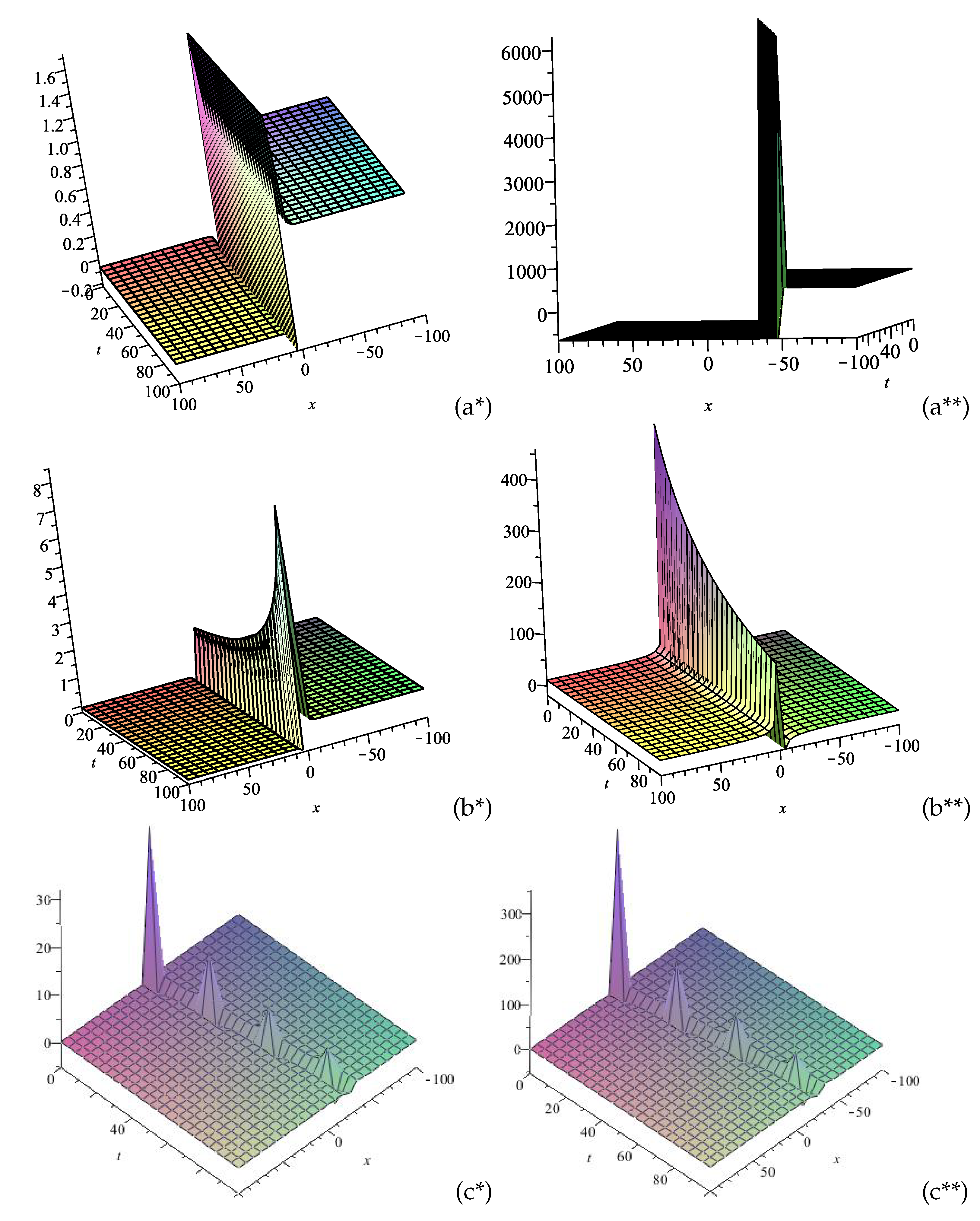
It is obvious that in the studied time-fractional predator-prey system, the corresponding population waves can demonstrate different dynamics than that of the classic predator-prey model. This is due to the choice of the model parameters, the diffusion rates and the strength of the Allee effect, which are particularly influenced by the fractional order. Bellow we shall present several illustrative examples of two solutions of Eqs (11) which can give a more realistic picture of specific population waves propagating in the modeled ecological medium. As it is seen from Figure 1(a*–b**), bistable waves moving from a low stable state, reaching a peak value, and then falling to another stable state are observed for both prey and predator populations. For the numerical simulations in Figure 1(a*,a**), only the influence of the Allee effect is accounted for (at $\varphi =1$). In this case, the population wave picture include low-density state, where both populations are near extinction or at very low levels, and high-density state, where both populations coexist at levels above the Allee thresholds, supported by mutual interactions. Thus, the wave fronts observed are characterized by a sharp rise in population densities as the waves move. Moreover, the prey population peaks first, followed by her predator because they propagate with different wave velocities. Next, the wave fronts transit back and are stabilized at a new (almost moderate) densities. In Figure 1(b*,b**), the combined effects of Allee threshold and fractional order on the propagating prey and predator population waves are shown. It is obvious, that the time–fractional order in the studied predator–prey system introduces a memory effect, meaning that past population states influence current growth rates. Thus, as it is seen from Figure 1(b*,b**), this memory effect slows down the rate of change in population densities, creating a smoother and more gradual wavefront compared to illustrative examples in Figure 1(a*,a**). In addition, for this case, the propagating population waves resemble single solitons. Although classical periodic waves are not typical for the studied population model due to the memory effect and the stabilizing influence of the Allee threshold, the system may display also damped or quasi-periodic oscillations which diminish over time (see Figure 1(c*,c**)). In this case, when the initial population densities of prey and predator exceed the Allee threshold, oscillations can occur, as both populations are large enough to interact meaningfully. The Allee effect, however, can leads also to damped oscillations, especially if the initial conditions are close to the Allee threshold. In these cases, oscillations may begin but gradually reduce in amplitude until the system settles into a stable state. In addition, the fractional order induces a memory effect, which leads to slowing oscillation frequency and creating smoother, longer-lasting oscillations as it is seen from Figure 1(c*,c**).

6. Conclusions

In this paper, we have presented all the possibilities offered by SEsM for finding exact solutions of systems of NPDEs and FNPDEs. The detailed SEsM algorithm proposed in the article outlines various step options depending on the nature of the modeled real-world process. This is crucial for obtaining a realistic understanding of the studied wave dynamics. In the specific case examined in the publication, we assumed that the predator and the prey populations in the predator-prey interaction model, considered, move at different wave speeds. From a practical point of view, this is a quite common situation in nature (for example, in animal populations). The new analytical solutions presented in the article, apart from their fundamental theoretical significance, also have partial practical applications through their numerical expressions. The last ones could assist biologists, ecologists and medical professionals in better understanding population dynamics, predicting interactions between species and developing strategies for ecosystem management and disease control.

References

- Rivero, M.; Trujillo, J. J.; Vázquez, L.; Velasco, M. P. Fractional dynamics of populations, Applied Mathematics and Computation 2011, 218 (3), 1089–1095. [CrossRef]
- Owolabi, K. M. High-dimensional spatial patterns in fractional reaction-diffusion system arising in biology. Chaos, Solitons & Fractals 2020, 134, 109723. [Google Scholar] [CrossRef]
- Ghanbari, B.; Günerhan, H.; Srivastava, H.M. An application of the Atangana-Baleanu fractional derivative in mathematical biology: A three-species predator-prey model. Chaos, Solitons & Fractals, 2020, 138, 109910. [Google Scholar] [CrossRef]
- Kulish, V. V.; Lage, J. L. Application of fractional calculus to fluid mechanics. J. Fluids Eng. 2002, 124(3), 803–806. [Google Scholar] [CrossRef]
- Yıldırım, A. Analytical approach to fractional partial differential equations in fluid mechanics by means of the homotopy perturbation method. International Journal of Numerical Methods for Heat & Fluid Flow 2010, 20 (2), 186–200.
- Hosseini, V. R.; Rezazadeh, A.; Zheng, H.; Zou, W. A nonlocal modeling for solving time fractional diffusion equation arising in fluid mechanics. Fractals, 2240. [Google Scholar] [CrossRef]
- Ozkan, E.M. New Exact Solutions of Some Important Nonlinear Fractional Partial Differential Equations with Beta Derivative. Fractal Fract., 2022, 6, 173. [Google Scholar] [CrossRef]
- Fallahgoul, H.; Focardi, S.; Fabozzi, F. Fractional calculus and fractional processes with applications to financial economics: Theory and application. Academic Press (2016).
- Ara, A.; Khan, N. A.; Razzaq, O. A.; Hameed, T.; Raja, M. A. Z. Wavelets optimization method for evaluation of fractional partial differential equations: an application to financial modelling. Advances in Difference Equations, 2018, 2018 (1), 1–13. [CrossRef]
- Tarasov, V. E. On history of mathematical economics: Applicatioactionaln of fr calculus. Mathematics 2019, 7(6), 509. [CrossRef]
- Kumar, S. A new fractional modeling arising in engineering sciences and its analytical approximate solution. 2013, 52 (4), 813–819. [CrossRef]
- Sun, H.; Zhang, Y.; Baleanu, D.; Chen, W.; Chen, Y. A new collection of real world applications of fractional calculus in science and engineering. Communications in Nonlinear Science and Numerical Simulation, 2018, 64, 213–231. [Google Scholar] [CrossRef]
- Chen, W., Sun, H. & Li, X. Fractional derivative modeling in mechanics and engineering. Springer Nature.(2022).
- The (G’G)-expansion method and travelling wave solutions of nonlinear evolution equations in mathematical physics.Physics Letters A 2008,372 (4), 417-423. [CrossRef]
- Zhang, J. & Li, Z. The F–expansion method and new periodic solutions of nonlinear evolution equations.Chaos, Solitons & Fractals, 2008, 37 (4), 1089–1096.
- Vitanov, N. K. On modified method of simplest equation for obtaining exact and approximate solutions of nonlinear PDEs: The role of the simplest equation. Communications in Nonlinear Science and Numerical Simulation, 2011, 16 (11), 4215–4231. [CrossRef]
- Vitanov, N.K. Application of Simplest Equations of Bernoulli and Riccati Kind for Obtaining Exact Traveling-Wave Solutions for a Class of PDEs with Polynomial non-linearity. Commun. Non-Linear Sci. Numer. Simul., 2010, 15 (7), 2050–2060. [CrossRef]
- Vitanov, N.K. Modified Method of Simplest Equation: Powerful Tool for Obtaining Exact and Approximate Traveling-Wave Solutions of non-linear PDEs. Commun. Non-Linear Sci. Numer. Simulation 2011, 16, 1176–1185. [Google Scholar] [CrossRef]
- Vitanov, N.K. On Modified Method of Simplest Equation for Obtaining Exact and Approximate Solutions of non-linear PDEs: The Role of the Simplest Equation. Commun. Non-Linear Sci. Numer. Simul. 2011, 16, 4215–4231. [Google Scholar] [CrossRef]
- Olver, P. J. Applications of Lie Groups to Differential Equations. Springer. (1986).
- Ibragimov, N. H. CRC Handbook of Lie Group Analysis of Differential Equations, Volumes I-III. CRC Press. (1994).
- Kevorkian, J. & Cole, J. D. Multiple Scale and Singular Perturbation Methods. Springer(1996).
- Nayfeh, A. H. Introduction to Perturbation Techniques. John Wiley & Sons (1981).
- Zhang, S. ; Zhang, H-Q. Fractional sub-equation method and its applications to nonlinear fractional PDEs,Physics Letters A, 2011, 375 (7), 1069–1073,. [CrossRef]
- Guo, S.; Mei, L.; Li, Y.; Sun, Y. The improved fractional sub-equation method and its applications to the space-time fractional differential equations in fluid mechanics. Phys. Lett. A, 2012, 376 (4), 407–411. [CrossRef]
- Lu, B. Backlund transformation of fractional Riccati equation and its applications to nonlinear fractional partial differential equations. Phys. Lett. A. 2012;376(28-29):2045–2048. [CrossRef]
- Adomian, G. A. review of the decomposition method in applied mathematics. Journal of Mathematical Analysis and Applications, 1990, 135 (2), 501–544. [CrossRef]
- Duan, J. S.; Rach, R. New higher-order numerical one-step methods based on the Adomian and the modified decomposition methods. Applied Mathematics and Computation 2011, 218(6), 2810–2828. [Google Scholar] [CrossRef]
- Vitanov, N.K. Simple equations method (SEsM) and nonlinear PDEs with fractional derivatives. AIP Conf. Proc. 2022, 2459, 030040. [Google Scholar] [CrossRef]
- Vitanov, N.K. Simple Equations Method (SEsM): An Effective Algorithm for Obtaining Exact Solutions of Nonlinear Differential Equations. Entropy, 2022, 24, 1653. [Google Scholar] [CrossRef]
- Vitanov, N. K. Vitanov, N. K. Simple equations method (SEsM): Review and new results. AIP Conference Proceedings, 2022, 2459 (1), 020003. [CrossRef]
- Vitanov, N.K. On the Method of Transformations: Obtaining Solutions of Nonlinear Differential Equations by Means of the Solutions of Simpler Linear or Nonlinear Differential Equations. Axioms, 2023, 12, 1106. [Google Scholar] [CrossRef]
- Nikolova, E.V. Exact Travelling-Wave Solutions of the Extended Fifth-Order Korteweg-de Vries Equation via Simple Equations Method (SEsM): The Case of Two Simple Equations. Entropy, 2022, 24, 1288. [Google Scholar] [CrossRef]
- Zhou, J.; Ju, L.; Zhao, S.; Zhang, Y. Exact Solutions of Nonlinear Partial Differential Equations Using the Extended Kudryashov Method and Some Properties. Symmetry, 2023, 15 (12), 2122. [CrossRef]
- Kudryashov, N.A.; Loguinova, N.B. Extended Simplest Equation Method for non-linear Differential Equations. Appl. Math. Comput. 2008, 205, 361–365. [Google Scholar] [CrossRef]
- Kudryashov, N.A. One Method for Finding Exact Solutions of non-linear Differential Equations. Commun. Non-Linear Sci. Numer. Simul. 2012, 17, 2248–2253. [Google Scholar] [CrossRef]
- Zhang, S.; Tong, J–L.; Wang, W. Exp-function method for a nonlinear ordinary differential equation and new exact solutions of the dispersive long wave equations, Computers & Mathematics with Applications 2009, 58 (11–12), 2294–2299. [CrossRef]
- Li, W–W. ; Tian, Y.; Zhang, Z. F-expansion method and its application for finding new exact solutions to the sine–Gordon and sinh-Gordon equations. Applied Mathematics and Computation 2012, 219(3), 1135–1143. [Google Scholar] [CrossRef]
- Hussain, A.; Chahlaoui, Y.; Zaman, F.D.; Parveen, T.; Hassan, A. M. The Jacobi elliptic function method and its application for the stochastic NNV system. Alexandria Engineering Journal 2023, 81, 347–359. [Google Scholar] [CrossRef]
- Khalil, R.; Al Horani, M.; Yousef, A.; Sababheh, M. A new definition of fractional derivative. Journal of Computational and Applied Mathematics, 2014, 264, 65–70. [Google Scholar] [CrossRef]
- Jumarie, G. Modified Riemann-Liouville derivative and fractional Taylor series of non-differentiable functions further results. Focuses on analytical methods using fractional transforms. Computers & Mathematics with Applications, 2006, 51 (9–10), 1367–1376. [CrossRef]
- lh2010) Li, Z.-B.; He, J.-H. Fractional Complex Transform for Fractional Differential Equations. Math. Comput. Appl., 2010, 15, 970–973. [Google Scholar] [CrossRef]
- Nikolova, E.V. Numerous Exact Solutions of the Wu-Zhang System with Conformable Time–Fractional Derivatives via Simple Equations Method (SEsM): The Case of Two Simple Equations. In: Slavova, A. (eds) New Trends in the Applications of Differential Equations in Sciences. NTADES 2023. Springer Proceedings in Mathematics & Statistics, 2024, 449. [CrossRef]
- Nikolov, R.G.; Nikolova, E.V.; Boutchaktchiev, V.N. Several Exact Solutions of the Fractional Predator—Prey Model via the Simple Equations Method (SEsM). In: Slavova, A. (eds) New Trends in the Applications of Differential Equations in Sciences. NTADES 2023. Springer Proceedings in Mathematics & Statistics, 2024, 449. [Google Scholar] [CrossRef]
- Nikolova, E.V. On the Traveling Wave Solutions of the Fractional Diffusive Predator—Prey System Incorporating an Allee Effect. In: Slavova, A. (eds) New Trends in the Applications of Differential Equations in Sciences. NTADES 2023. Springer Proceedings in Mathematics & Statistics, 2024, 449. [Google Scholar] [CrossRef]
- Li, C.; Deng, W. Remarks on fractional derivatives. Applied Mathematics and Computation 2007, 187, 777–784. [Google Scholar] [CrossRef]
- Nikolova, E.V.; Dimitrova, Z.I. Exact taveling wave solutions of a generalized Kawahara equation. J. Theor. Appl. Mech., 2019, 49, 123–135. [Google Scholar] [CrossRef]
Figure 1.
The wave behaviour of (the left column) and (the right column) based on numerical simulations of Eqs (35) at and: (a*) and (a**) for ; (b*) and (b**) for ; (c*) and (c**): The wave behaviour of (the left column) and (the right column) based on numerical simulations of Eqs (40) at .
Disclaimer/Publisher’s Note: The statements, opinions and data contained in all publications are solely those of the individual author(s) and contributor(s) and not of MDPI and/or the editor(s). MDPI and/or the editor(s) disclaim responsibility for any injury to people or property resulting from any ideas, methods, instructions or products referred to in the content. |
© 2024 by the authors. Licensee MDPI, Basel, Switzerland. This article is an open access article distributed under the terms and conditions of the Creative Commons Attribution (CC BY) license (http://creativecommons.org/licenses/by/4.0/).
Copyright: This open access article is published under a Creative Commons CC BY 4.0 license, which permit the free download, distribution, and reuse, provided that the author and preprint are cited in any reuse.