
Submitted:
02 December 2024
Posted:
04 December 2024
You are already at the latest version
Abstract
In the present paper, several viscoelastic models are studied for the cases when time-dependent viscoelastic operators are represented in terms of the fractional derivative Kelvin-Voigt, Scott Blair, Maxwell, and standard linear solid models. Using the algebra of dimensionless Rabotnov’s fractional exponential functions, time-dependent operators for Poisson’s ratios have been obtained and analyzed. It is shown that materials described by some of such models are viscoelastic auxetics, because Poisson’s ratios of such materials are time-dependent operators which could take on both positive and negative magnitudes.
Keywords:
viscoelastic materials
; auxetics
; wave propagation
; fractional calculus
; Rabotnov fractional exponential function
MSC: 35C07; 35D40; 3Q74; 74D0; 74J10
1. Introduction
It is known [1] that pure elastic bodies do not exist in nature. All media possess viscoelastic features to one degree or another, and their main physical-and-mechanical properties are time-dependent. Due to wide application of the theory of elasticity in studies of advanced and traditional materials, much attention is given to modelling and investigative techniques of viscoelastic media and bodies subjected to various types of loading [1,2,3,4,5].
During the last three decades Fractional Calculus has gained wide acceptance in modelling such viscoelastic bodies as beams, plates, and shells [6,7]. Their damping features are described most often by defining the Young’s operator by the simplest fractional derivative models, namely: Kelvin-Voight model, Maxwell model, and standard linear solid model [8,9,10]. As this takes place, the Poisson’s ratio of a viscoelastic material is frequently assumed to be a constant [11,12]. However, it has been emphasized in [13] that the fractional derivative Kelvin-Voigt model with a time-independent Poisson’s ratio is only acceptable for the description of the dynamic behaviour of elastic bodies in a viscoelastic medium [6,14,15] or on a viscoelastic foundation[16].
As experimental data have shown [17], the Poisson’s ratio is always a time-dependent operator [18,19,20], and only the bulk extension-compression operator could be considered as a constant value, since for the most viscoelastic materials it varies weakly during deformation [1,2].
The detailed reviews of `traditional’ fractional calculus models in viscoelasticity (`traditional’ in the sense that such models consider time-independent Poisson’s ratios) are given in [6,10,13,21]. In the present paper, the fractional derivative models involving the time-dependent Poisson’s operators will be studied, which allows one to reveal rather interesting properties of advanced viscoelastic materials, among them auxetic materials possessing negative Poisson’s ratios [22,23,24,25].
For solving different dynamic problems of mechanics of viscoelastic solids and structures, it is essential to know the form of viscoelastic operators entering in governing equations. For example, Poisson’s ratio and Young’s modulus are involved in the cylindrical rigidity of plates and shells, and therefore in the Hertz’s law for the solution of the problem of viscoelastic contact interaction during impact [26,27,28]. Therefore, their pinpointing is of paramount importance in the impact response analysis.
It is well known [29,30] that each isotropic elastic material possesses only two independent material constants, and all others are expressed in terms of two constants that should be preassigned or determined experimentally. Possible combinations are presented in Table 1, where two prescribed constants are shown in the first column, while the others are determined in terms of two given constants according to formulas, which are located at the intersections of the corresponding lines and columns.
From Table 1 it is seen that for materials, the bulk relaxation of which could be neglected, i.e., to consider K as a constant value, two independent material moduli could be assigned via four ways.
Similarly, in the case of isotropic viscoelastic media, material properties are time-dependent and are described by operators, which should be expressed in terms of two preassigned ones (or determined from experimental data) utilizing the correspondence principle and relationships given in Table 1.
For solving one-dimensional dynamic problems of viscoelasticity, it is a need to know the Young’s and shear operators defining phase velocities and coefficients of attenuation of viscoelastic longitudinal and shear waves. Thus, modelling of these time-dependent operators without volume relaxation (K = const) has been considered using the following viscoelastic fractional derivative models:
Interestingly to note that only the first and second Lamé constants,λ and µ, or the bulk and shear moduli, K and µ, appear in Hooke’s law for three-dimensional media, but not Young’s modulus E, or Poisson’s ratio . This indicates that K, and µ are the most intrinsic operators to express stress in terms of strain when studying wave propagation in 3D viscoelastic media [38,39,40].
That is why in the present paper, the emphasis will be make on the comprehensive analysis of time-dependent operators for Lamé parameters. Using the procedure for the study of viscoelastic operators suggested in Rossikhin and Shitikova [13,34], below for the first time the models based on the application of fractional derivatives will be studied for the cases when the first Lame parameter or the P-wave modulus is given a priori, without considering the bulk relaxation.
2. Models of Viscoelasticity Involving Fractional Order Operators With Time-Dependent Poisson’s Ratio
2.1. Preliminary Remarks
The rheological equations of the simplest fractional derivative models of viscoelasticity widely used in mechanics are the following [10,13]:
or
where σandε are the stress and the strain, respectively, and are the relaxation and retardation (or creep) times, respectively, and are the nonrelaxed (instantaneous) and relaxed (prolonged) moduli of elasticity, , is the defect of the modulus, i.e. the value characterizing the decrease in the elastic modulus from its nonrelaxed value to its relaxed magnitude, is the Riemann-Liouville fractional derivative [41] of the order
is the Gamma-function, () is the dimensionless Rabotnov’s operator [9,34], and is the fractional exponential function [1,2], which at goes over into a conventional exponential function.
It is known [13] that both versions of the standard linear solid model shown in Figure 1D and Figure 1E are described by one and the same equation (4), wherein model parameters are interconnected by the following relationship:
Equations (2)-(6) govern stress-strain relationships for one-dimensional viscoelastic media. The constitutive equation connecting the strain and stress in a linear viscoelastic isotropic medium has the form
or
where and are stress and strain tensors components, , and are, respectively, time-dependent Lamé and bulk operators, and is the Kronecker delta.
Thus, for solving three-dimensional dynamic problems of viscoelasticity, it is a need to know the form of two time-dependent operators: and , or and .
Below we will consider models involving time-dependent Poisson’s ratio but without volume relaxation, i.e. when bulk modulus is time-independent (this assumption is due to the fact that for many viscoelastic materials volumetric relaxation is much smaller than the shear relaxation)
where is a certain constant which could take on the value of nonrelaxed bulk modulus or relaxed bulk modulus , and is the identity operator.
Therefore, it is necessary to assign the second operator, i.e., one of the Lamé operators or , or P-wave operator , what could be done using the fractional derivative Maxwell, Scott Blair, Kelvin-Voigt, or standard linear solid models (2)-(6). Knowing the form of two viscoelastic operators, it is possible to define the form of the time-dependent Poisson’s operator and all other operators.
2.2. Modelling of the Shear Operator Using the Fractional Derivative Kelvin-Voigt Model
The shear operator is most frequently preassigned via the fractional derivative Kelvin-Voigt model (4) as
where is the relaxed shear modules, is the retardation time during shear deformations, while the bulk operator is assumed to be constant according to (11).
In order to evaluate dynamic response of viscoelastic bodies, for example, impact response, it is necessary to calculate the Young’s operator. For this purpose using the Volterra principle and formula from the third line in Table 1:
First we could write the operator
where .
Then we find the operator reverse to (14), i.e.,
Now the Poisson’s operator could be calculated via the following formula:
From relationship (20) the limiting magnitudes of the Poisson’s ration could be calculated
2.3. Modelling the Shear Operator Using the Fractional Derivative Maxwell Model
If the fractional derivative Maxwell model (3) is applied for describing viscoelastic bodies, then the shear operator could be written in the form
where is the nonrelaxed magnitude of the shear modulus, in so doing the volumetric operator is still considered as a constant .
Using the procedure described above for the Kelvin-Voigt model, we could similarly obtain for the Maxwell model
or
where is the nonrelaxed magnitude of the Poisson’s ratio.
Then the Poisson’s operator will take the form
whence the limiting values of the operator are the following:
From relationships (27) it is seen that for the fractional derivative Maxwell model, Poisson’s ratio could increase from to its limiting value of 0.5, what means that this model is suitable for the analysis of viscoelastic rubber-like materials.
2.4. Scott Blair Model for Shear Relaxation
Some authors prefer to use the simplest fractional derivative model, i.e., the Scott Blair element (1) for modelling the shear operator
and assume that volumetric relaxation is absent, i.e. , where .
In this case
Then the Poisson’s operator takes the form
whence it follows that
From (32) it is evident that according to this model the Poisson’s ratio could vary in a very broad range, namely, form -1 to 0.5. Thus, this model is thermodynamically admissible for viscoelastic auxetics.
2.5. Modelling the Shear Operator Via the Fractional Derivative Standard Linear Solid Model
If the fractional derivative standard linear solid model (6) is applied for describing viscoelastic bodies, then the shear operator has the form
or
Substituting (16) in (34) and introducing the notation (similar to relationship (8))
yield
where , in so doing operator is still defined by (11).
For this model the time-dependent Poisson’s operator will take the form
or
From relationship (38) it is seen that the limiting values of the Poisson’s ratio, i.e. nonrelaxed and relaxed magnitudes, are the following:
Thus, the model (36) allows one to describe both the relaxation and creep processes of viscoelastic materials, and it could be applied for solving different dynamics problems.
2.6. Modelling the Relaxation of the First Lamé parameter Via the Fractional Derivative Standard Linear Solid Model
Now let us consider the case when the first Lamé parameter is preassigned by the fractional derivative standard linear solid model (6):
where the nonrelaxed and relaxed moduli of the first Lamé parameter are connected with the relaxation and retardation times similar to (8) by the relationship
and .
For the model under consideration with and K defined by relationships (40) and (11), respectively, in so doing , the time-dependent Poisson’s operator according to line 2 in Table 1 is expressed as follows:
or
Then the time-dependence of the Poisson’s ratio and its nonrelaxed and relaxed magnitudes could be obtained from relationship (42) in the form
Reference to (44) shows that this model describes the behaviour of viscoelastic materials, the Poisson’s ratio of which varies with time from to .
2.7. Modelling the P-Wave Modulus Via Fractional Derivative Standard Linear Solid Model
One of the most efficient methods of the reconstruction of the material parameters of a linear isotropic viscoelastic structure is from time-dependent measurements of a viscoelastic wave on the surface of a bounded domain of propagation [39]. In this case, the combination of both Lamé parameters, which is called as the modulus of the longitudinal wave, or P-wave, could be preassigned .
Assume that operator is given by the fractional derivative standard linear solid model (4):
where the nonrelaxed and relaxed magnitudes of the P-wave modulus are connected with the relaxation and retardation times similar to (8) by the relationship
and .
For the model under consideration with and K defined by relationships (47) and (11), respectively, the time-dependent Poisson’s operator according to the last line in Table 1 is expressed as follows:
or
Then the time-dependence of the Poisson’s ratio and its nonrelaxed and relaxed magnitudes could be obtained from relationship (47) in the form
From (49) it is seen that similar to the cases, when each of the Lamé parameters is defined separately by the fractional derivative standard linear solid, modelling the P-wave modulus allows one to describe the behaviour of viscoelastic materials, Poisson’s ratio of which varies with time from its nonrelaxed value to its relaxed value.
3. Analysis of the Fractional Derivative Models of Viscoelasticity Involving Time-Dependent Poisson’s Ratio and Without Volume Relaxation
From Table 1 it is seen that for viscoelastic materials, the volume relaxation of which could be neglected, i.e., bulk modulus could be considered as a constant value , as a second time-dependent operator which should be given together with one of the four material characteristics could be preassigned: E, , , or . In its turn, each of these operators could be described by four fractional derivative models: Scott Blair, Kelvin-Voigt, Maxwell, or standard linear solid models. Thus, there could be 16 different variants of viscoelastic models involving time-dependent Poisson’s ratio, seven of which have been considered above in Section 2, and some models are presented in [13,31,32,33,34].
The limiting values of the time-dependent Poisson’s ratio are summarized in Table 2Table 3 for all 16 models, what will allow one to classify the models constructed.
- 1.
- models describing the behaviour of ’traditional’ viscoelastic isotropic materials, i.e., materials with positive magnitudes of Poisson’s ratio within the thermodynamically admissible range – models No. 3, 4, 7, 8, 11, 12, 16;
- 2.
- models describing the behaviour of isotropic viscoelastic materials with negative Poisson’s ratios within the thermodynamically admissible range – models No. 5, 6, 9, 10, 14;
- 3.
- physically meaningless models, i.e., models with Poisson’s ratios lying without the thermodynamically admissible domain either from the left with – models 1 and 2, or from the right with – models 13 and 15.
The fractional derivative standard linear solid model, which could describe both the relaxation and creep phenomena occurring during deformation of viscoelastic materials, provides the variation of Poisson’s ratio with time from its nonrelaxed (instantaneous) magnitude to its relaxed (prolonged) magnitude according to the relationship similar in the form to all models:
in so doing the limiting values of Poisson’s ratios are calculated for each model individually.
The time-dependence of the Poisson’s ratio for fractional derivative standard linear solid models for Lamé parameters: model 8 for (26), model 12 for (44), and model 16 for (49) are presented in Figure 2 for and at different values of the fractional parameter , and 1, whence it is evident that all curves increase monotonically from 0.25 to 0.3, and the curve corresponding to approaches the upper limit more rapidly than the curves for fractional magnitudes of .
The Maxwell models for Young’s operator (model 3) and for shear operator (model 7) behave in a similar way: Poisson’s ratio varies with time from its nonrelaxed magnitude to 1/2, as it is shown in Figure 3.
Scott Blair models for the shear operator (model 5) and the first Lamé operator (model 9), Kelvin-Voigt models for the shear operator (model 6), the first Lamé operator (model 10), and the P-wave operator (model 14) describe the behaviour of viscoelastic auxetics with the lower limit of the Poisson’s ratio equal to . As for the upper limiting magnitude of the Poisson’s ratio, then for the model 5 it is 1/2, for the model 9 it is zero, and for the models 6, 10, and 14, it is a finite value within the range of , which depends on the given magnitudes of the preassigned operators. Time-dependence of the Poisson’s operator for the model 14 is shown in Figure 4.
4. Conclusion
In the present paper, several viscoelastic models are studied for the cases when time-dependent viscoelastic operators are represented in terms of the fractional derivative Scott Blair, Kelvin-Voigt, Maxwell, and standard linear solid models. Using the algebra of dimensionless Rabotnov’s fractional exponential functions, time-dependent operators for Poisson’s ratios have been obtained and analyzed. It is shown that materials described by some of such models are viscoelastic auxetics, because Poisson’s ratios of such materials are time-dependent operators which could take on both positive and negative magnitudes.
In the companion paper, it is planned to analyze viscoelastic materials involving time-dependent operators, including the Poisson’s operator with due account for bulk relaxation.
Author Contributions
All authors have contributed equally. All authors have read and agreed to the published version of the manuscript.
Funding
This research was supported by National Research Moscow State University of Civil Engineering (grant No. 36-392/130).
Data Availability Statement
The data used to support the findings of this study are available from the corresponding author upon reasonable request.
Conflicts of Interest
The authors declare no conflict of interest.
References
- Rabotnov, Yu.N. Creep Problems in Structural Members; North-Holland: Amsterdam, 1969. [Google Scholar]
- Rabotnov, Yu.A. Elements of Hereditary Solid Mechanics; Nauka: Moscow, 1980. [Google Scholar]
- Christensen, R.M. Theory of Viscoelasticity. An Introduction; Academic Press: New York and London, 1971. [Google Scholar]
- Bland, D.R. The Theory of Linear Viscoelasticity; Pergamon Press: New York, 1960. [Google Scholar]
- Tschoegl, N.W. The Phenomenological Theory of Linear Viscoelastic Behavior; Springer: Berlin, 1989. [Google Scholar]
- Rossikhin, Y.A.; Shitikova, M.V. Application of fractional calculus for dynamic problems of solid mechanics: Novel trends and recent results. Appl. Mech. Rev. 2010, 63, 010801. [Google Scholar] [CrossRef]
- Rossikhin, Y.A.; Shitikova, M.V. Fractional calculus in structural mechanics. In Handbook of Fractional Calculus with Applications, Vol. 7, Applications in Engineering, Life and Social Sciences, Part A; Baleanu, D., Lopes, A.M., Eds.; De Gruyter: Berlin, Boston, 2019; pp. 159–192. [Google Scholar]
- Rossikhin, Y.A.; Shitikova, M.V. Applications of fractional calculus to dynamic problems of linear and nonlinear hereditary mechanics of solids. Appl. Mech. Rev. 1997, 50, 15–67. [Google Scholar] [CrossRef]
- Rossikhin, Y.A.; Shitikova, M.V. Fractional calculus models in dynamic problems of viscoelasticity. In Handbook of Fractional Calculus with Applications, Vol. 7, Applications in Engineering, Life and Social Sciences, Part A; Baleanu, D., Lopes, A.M., Eds.; De Gruyter: Berlin, Boston, 2019; pp. 139–158. [Google Scholar]
- Shitikova, M.V.; Krusser, A.I. Models of viscoelastic materials: a review on historical development and formulation. Adv. Struct. Mat. 2022, 175, 285–326. [Google Scholar]
- Atanacković, T.M.; Pilipović, S.; Stanković, B.; Zorica, D. Fractional Calculus with Applications in Mechanics: Wave Propagation, Impact and Variational Principles; Wiley: London, 2014. [Google Scholar]
- Schiessel, H.; Metzler, R.; Blumen, A.; Nonnenmacher, T.F. Generalized viscoelastic models: their fractional equations with solutions. J. Phys. A: Math Gen. 1995, 28, 6567–6584. [Google Scholar] [CrossRef]
- Shitikova, M.V. Fractional operator viscoelastic models in dynamic problems of mechanics of solids: a review. Mech. Solids 2022, 57, 1–33. [Google Scholar] [CrossRef]
- Rossikhin, Y.A.; Shitikova, M.V.; Estrada, M.M.G. Modeling of the impact response of a beam in a viscoelastic medium. Appl. Math. Sci. 2016, 10, 2471–2481. [Google Scholar] [CrossRef]
- Rossikhin, Y.A.; Shitikova, M.V.; Trung, P.T. Application of the fractional derivative Kelvin-Voigt model for the analysis of impact response of a Kirchhoff-Love plate. WSEAS Trans. Math. 2016, 15, 498–501. [Google Scholar]
- Spanos, P.D.; Malara, G. Nonlinear random vibrations of beams with fractional derivative elements. J. Eng. Mech. 2014, 140, 04014069. [Google Scholar] [CrossRef]
- Hilton, H.H. The elusive and fickle viscoelastic Poisson’s ratio and its relation to the elastic-viscoelastic correspondence principle. J. Mech. Mat. Struct. 2009, 4, 1341–1364. [Google Scholar] [CrossRef]
- Hilton, H.H. Implications and constraints of time-independent Poisson ratios in linear isotropic and anisotropic viscoelasticity. J. Elasticity 2001, 63, 221–251. [Google Scholar] [CrossRef]
- Hilton, H.H. Clarifications of certain ambiguities and failings of Poisson’s ratios in linear viscoelasticity. J. Elasticity 2011, 104, 303–318. [Google Scholar] [CrossRef]
- Tschoegl, N.W.; Knauss, W.G.; Emri, I. Poisson’s ratio in linear viscoelasticity - a critical review. Mech. Time-Depend. Mat. 2002, 6, 3–51. [Google Scholar] [CrossRef]
- Mainardi, F.; Spada, G. Creep, relaxation and viscosity properties for basic fractional models in rheology. Eur. Phys. J. Special Topics 2011, 193, 133–160. [Google Scholar] [CrossRef]
- Bhullar, S.K. Three decades of auxetic polymers: a review. E-Polymers 2015, 15, 205–215. [Google Scholar] [CrossRef]
- Carneiro, V.H.; Meireles, J.; Puga, H. Auxetic materials - A review. Materials Science-Poland 2013, 31, 561–571. [Google Scholar] [CrossRef]
- Mazaev, A.V.; Ajeneza, O.; Shitikova, M.V. Auxetics materials: classification, mechanical properties and applications. In IOP Conf. Ser.: Mat. Sci. Eng. 2020, 747, 012008. [Google Scholar] [CrossRef]
- Seyedkazemi, M.; Wenqi, H.; Jing, G.; Ahmadi, P.; Khajehdezfuly, A. Auxetic structures with viscoelastic behavior: A review of mechanisms, simulation, and future perspectives. Structures 2024, 70, 107610. [Google Scholar] [CrossRef]
- Rossikhin, Y.A.; Shitikova, M.V. Two approaches for studying the impact response of viscoelastic engineering systems: An overview. Comp. Math. Appl. 2013, 66, 755–773. [Google Scholar] [CrossRef]
- Shitikova, M.V. Impact response of a viscoelastic plate made of a material with negative Poisson’s ratio. Mech. Adv. Mat. Struct. 2022, 30, 982–994. [Google Scholar] [CrossRef]
- Teimouri, H.; Faal, R.T.; Milani, A.S. Impact response of fractionally damped rectangular plates made of viscoelastic composite materials. Appl. Math. Model. 2025, 137, 115678. [Google Scholar] [CrossRef]
- Love, A.E.H. A Treatise on the Mathematical Theory of Elasticity; Cambridge University Press: Cambridge, 1892. [Google Scholar]
- Landau, L.D.; Lifshits, E.M. Mechanics of Continua: Hydrodynamics and Theory of Elasticity; OGIZ: Moscow-Leningrad, 1944 (in Russian).
- Rossikhin, Y.A.; Shitikova, M.V.; Krusser, A.I. To the question on the correctness of fractional derivative models in dynamic problems of viscoelastic bodies. Mech. Res. Com. 2016, 77, 44–49. [Google Scholar] [CrossRef]
- Rossikhin, Y.A.; Shitikova, M.V. The fractional derivative Kelvin-Voigt model of viscoelasticity with and without volumetric relaxation. J. Phys.: Conf. Ser. 2018, 991, 012069. [Google Scholar] [CrossRef]
- Modestov, K.A.; Shitikova, M.V. Harmonic wave propagation in viscoelastic media modelled via fractional derivative models. Izv. Saratov Univ. Math. Mech. Inform. 2025, 25, 1–18. [Google Scholar]
- Rossikhin, Y.A.; Shitikova, M.V. Features of fractional operators involving fractional derivatives and their applications to the problems of mechanics of solids. In Fractional Calculus: History, Theory and Applications; Daou, R., Xavier, M., Eds.; Nova Science Publishers: New York, 2015; pp. 165–226. [Google Scholar]
- Zhu, Z.Y.; Li, G.G.; Cheng, C.J. Quasi-static and dynamical analysis for viscoelastic Timoshenko beam with fractional derivative constitutive relation. Appl. Math. Mech. 2002, 23, 1–12. [Google Scholar]
- Makris, N. Three-dimensional constitutive viscoelastic laws with fractional order time derivatives. J. Rheol. 1997, 41, 1007–1020. [Google Scholar] [CrossRef]
- Levin, V.; Sevostianov, I. Micromechanical modeling of the effective viscoelastic properties of inhomogeneous materials using fractional-exponential operators. Int. J. Fract. 2005, 134, L37–L44. [Google Scholar] [CrossRef]
- Ji, S.; Sun, S.; Wang, Q.; Marcotte, D. Lamé parameters of common rocks in the Earth’s crust and upper mantle. J. Geophys. Res. 2010, 115, B06314. [Google Scholar] [CrossRef]
- Lechleiter, A.; Schlasche, J.W. Identifying Lamé parameters from time-dependent elastic wave measurements. Inverse Problems in Science and Engineering 2017, 25, 2–26. [Google Scholar] [CrossRef]
- Holm, S. Waves with Power-Law Attenuation; Springer: Cham, 2019. [Google Scholar]
- Samko, S.G.; Kilbas, A.A.; Marichev, O.I. Fractional Integrals and Derivatives and Some of Their Applications; Nauka i Tekhnika: Minsk, 1987. [Google Scholar]
Figure 1.
Schemes of the rheological fractional derivatives models: Scott Blair model (A), Maxwell model (B), Kelvin–Voigt model (C), Poynting–Thomson–Ishlinsky model (D), Zener–Rzhanitsyn model (E).
Figure 1.
Schemes of the rheological fractional derivatives models: Scott Blair model (A), Maxwell model (B), Kelvin–Voigt model (C), Poynting–Thomson–Ishlinsky model (D), Zener–Rzhanitsyn model (E).
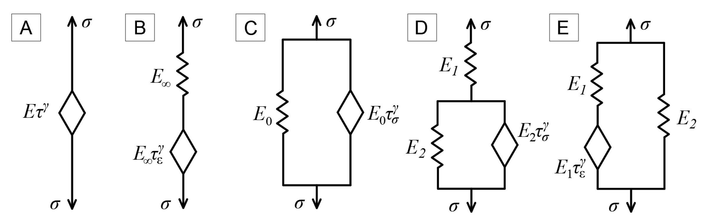
Figure 2.
Time-dependence of the Poisson’s ratio for fractional derivative standard linear solid models 8 (26), 12 (44), and 16 (49)
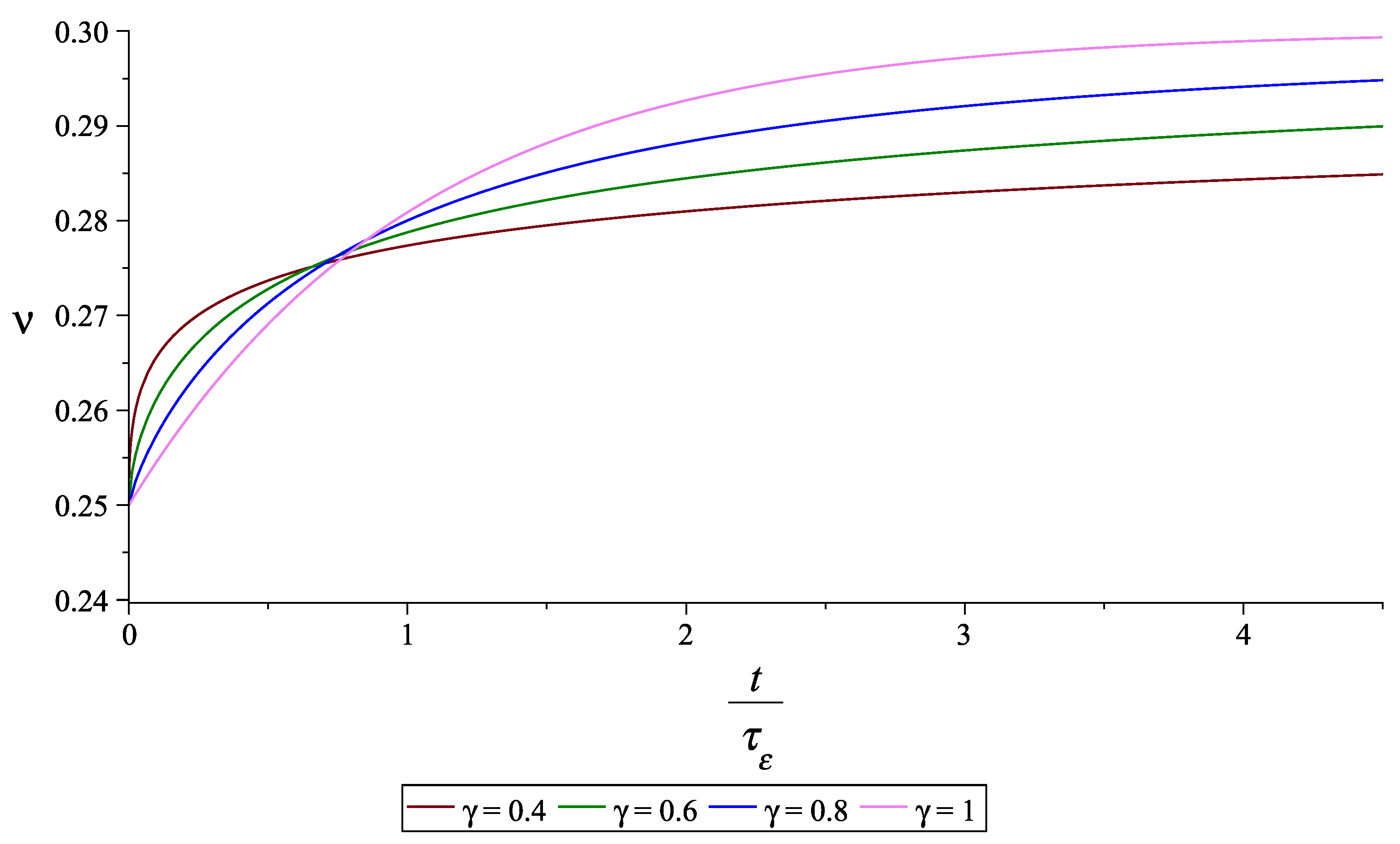
Figure 3.
Time-dependence of the Poisson’s ratio for the Maxwell model for Young’s operator (model 3 in Table 2.
Figure 3.
Time-dependence of the Poisson’s ratio for the Maxwell model for Young’s operator (model 3 in Table 2.
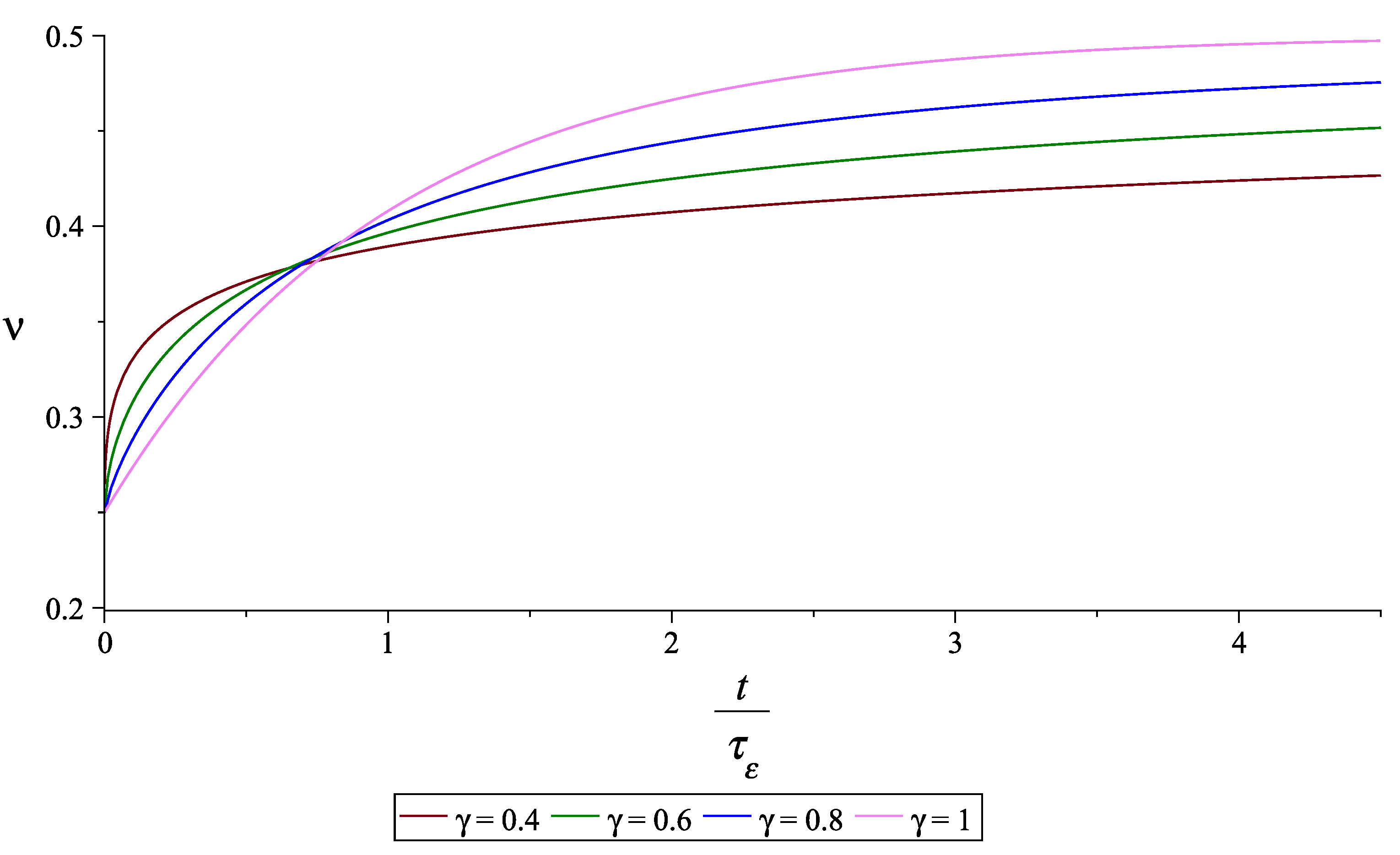
Figure 4.
Time-dependence of the Poisson’s ratio for the model 14.
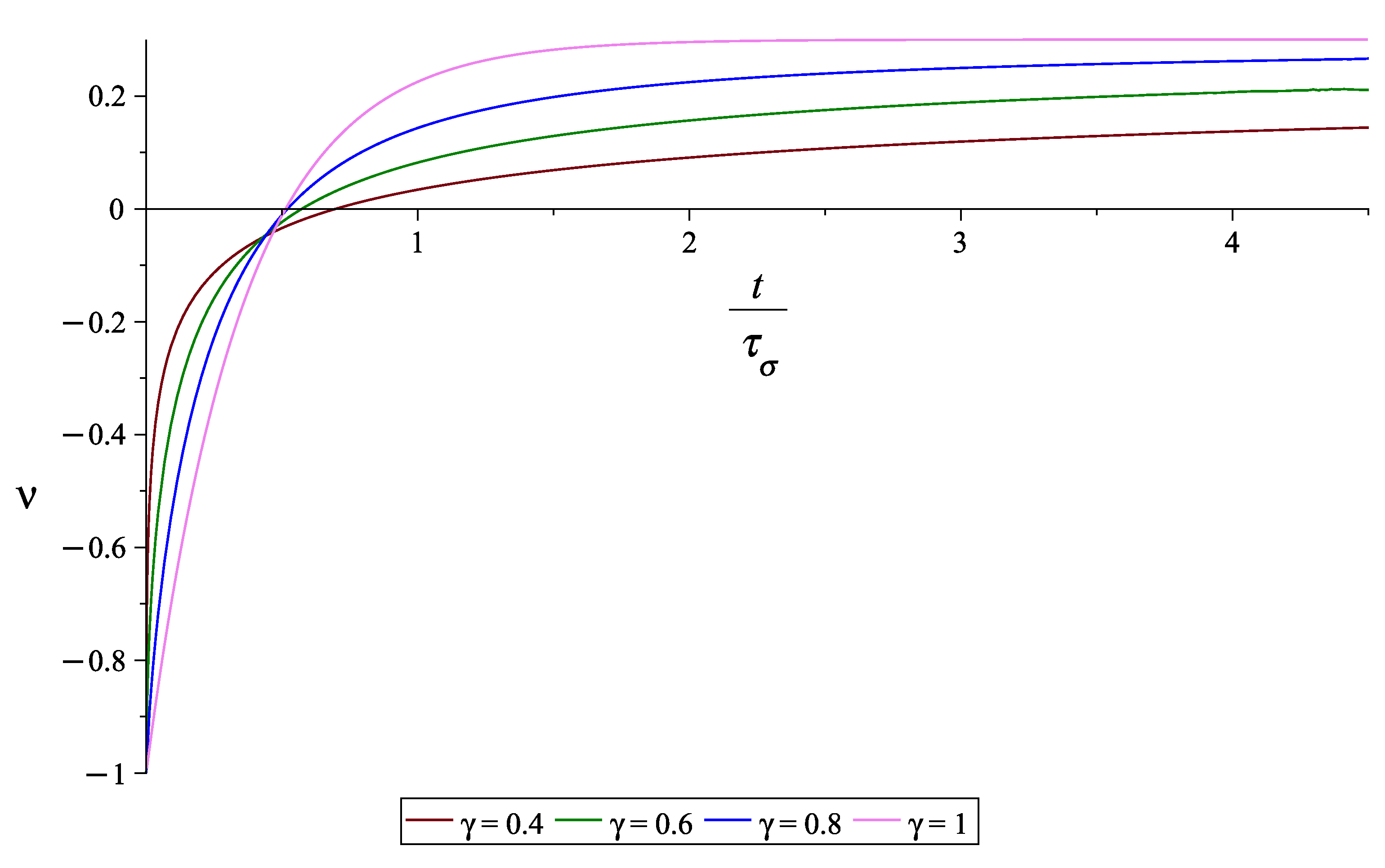
Figure 5.
Time-dependence of the Poisson’s ratio for the model 11 if .
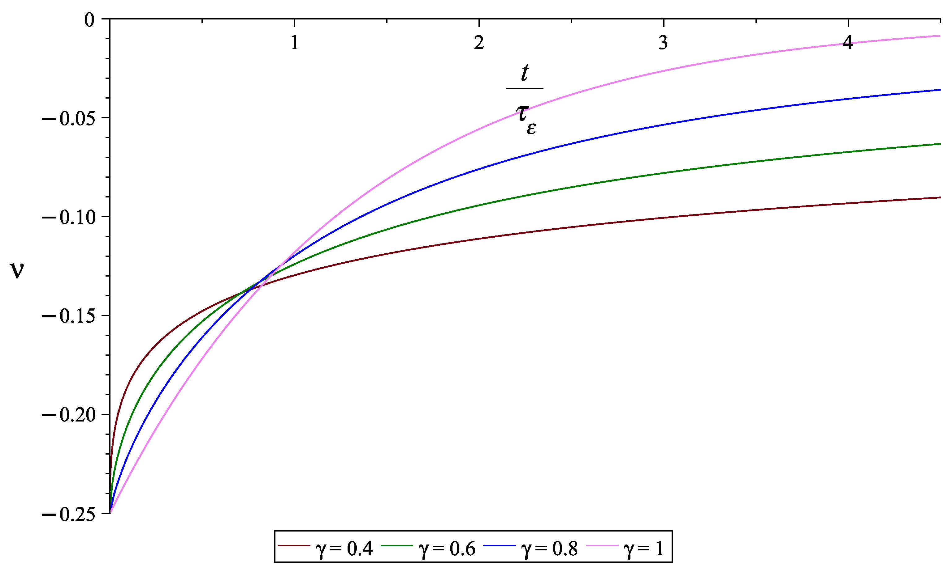
Figure 6.
Time-dependence of the Poisson’s ratio for the model 11 at .
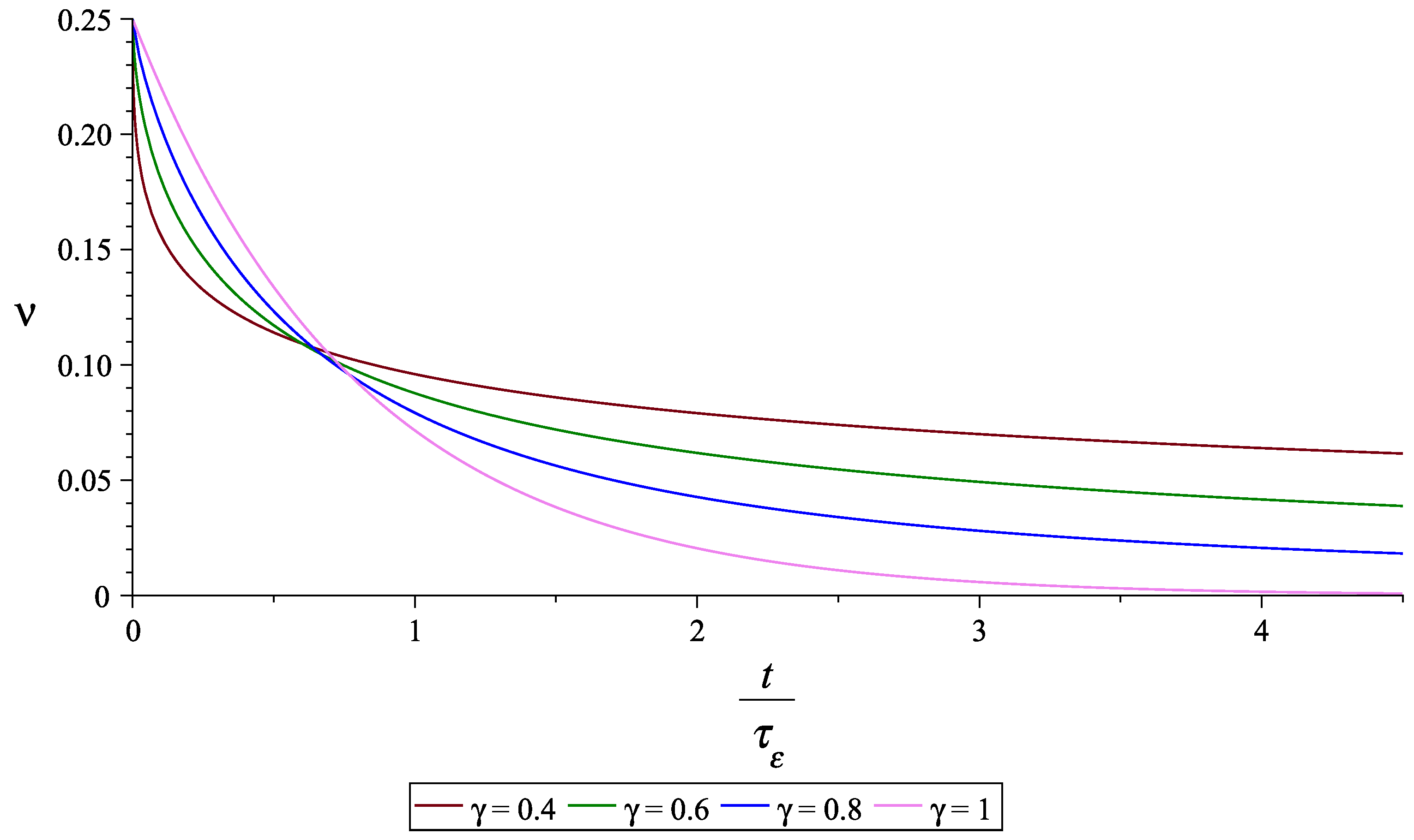
Figure 7.
Time-dependence of the Poisson’s ratio for the model 2.
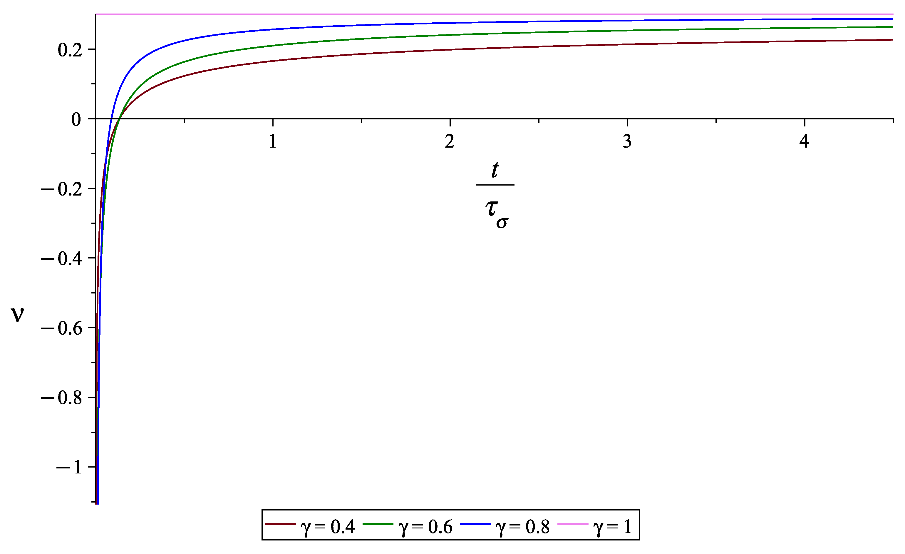
Figure 8.
Time-dependence of the Poisson’s ratio for the model 15.
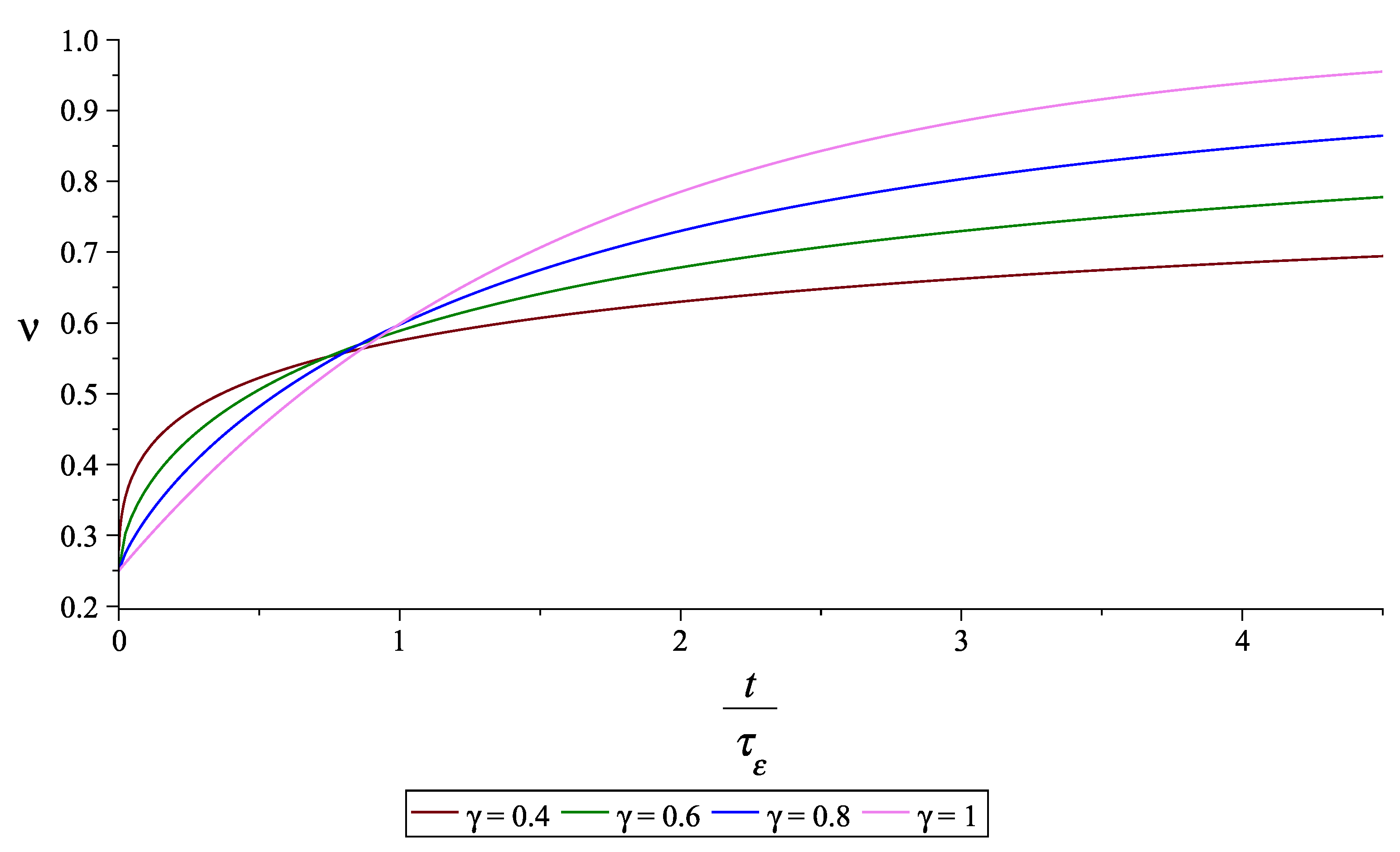

Table 1.
The interrelationship of elastic material constants: bulk modulus K, Young’s modulus E, Lamé’s parameters and , Poisson’s ratio , and P-wave modulus M.
Table 1.
The interrelationship of elastic material constants: bulk modulus K, Young’s modulus E, Lamé’s parameters and , Poisson’s ratio , and P-wave modulus M.
| Material constants | Young’s modulus E | 1st Lamé’s parameter | Shear modulus | Poisson’s ratio | P-Wave modulus M |
|---|---|---|---|---|---|
| - | |||||
| - | |||||
| - | |||||
| - | |||||
| - |
Table 2.
Limiting values of the Poisson’s ratio for isotropic materials, viscoelastic features of which are described by by different fractional-order operators without bulk relaxation (Part 1).
Table 2.
Limiting values of the Poisson’s ratio for isotropic materials, viscoelastic features of which are described by by different fractional-order operators without bulk relaxation (Part 1).
| Type of the model involving fractional derivatives | ||
|---|---|---|
| A. Modelling the Young’s operator | ||
| 1) Scott Blair model | ||
| 2) Kelvin-Voigt model | ||
| 3) Maxwell model | ||
| 4) Standard linear solid model | ||
| B. Modelling the shear operator (second Lamé parameter parameter) | ||
| 5) Scott Blair model | ||
| 6) Kelvin-Voigt model | ||
| 7) Maxwell model | ||
| 8) Standard linear solid model | ||
Table 3.
Limiting values of the Poisson’s ratio for isotropic materials, viscoelastic features of which are described by by different fractional-order operators without bulk relaxation (Part 2).
Table 3.
Limiting values of the Poisson’s ratio for isotropic materials, viscoelastic features of which are described by by different fractional-order operators without bulk relaxation (Part 2).
| Type of the model involving fractional derivatives | ||
|---|---|---|
| C. Modelling of the first Lamé parameter parameter | ||
| 9) Scott Blair model | ||
| 0 | ||
| 10) Kelvin-Voigt model | ||
| 11) Maxwell model | ||
| 0 | ||
| 12) Standard linear solid model | ||
| D. Modelling the P-wave modulus operator | ||
| 13) Scott Blair model | ||
| 1 | ||
| 14) Kelvin-Voigt model | ||
| 15) Maxwell model | ||
| 1 | ||
| 16) Standard linear solid model | ||
Disclaimer/Publisher’s Note: The statements, opinions and data contained in all publications are solely those of the individual author(s) and contributor(s) and not of MDPI and/or the editor(s). MDPI and/or the editor(s) disclaim responsibility for any injury to people or property resulting from any ideas, methods, instructions or products referred to in the content. |
© 2024 by the authors. Licensee MDPI, Basel, Switzerland. This article is an open access article distributed under the terms and conditions of the Creative Commons Attribution (CC BY) license (http://creativecommons.org/licenses/by/4.0/).
Copyright: This open access article is published under a Creative Commons CC BY 4.0 license, which permit the free download, distribution, and reuse, provided that the author and preprint are cited in any reuse.


