Short-term Vegetation Stress Monitoring Mapping With Machine Learning

1. Introduction

Vegetation stress is caused as a result of negative environmental effects on the health of a plant. Unfavorable environmental conditions affect plants’ metabolism, growth or development (Niemann and Visintini, 2005). When plants are subjected to less than ideal conditions required for their growth, they tend to be under stress. Vegetation stress can be induced by various natural and anthropogenic stress factors. Thus a differentiation can be made between short and long time stress effect as well as between low stress events which can be partially compensated for, by accumulation, adaptation and repair mechanisms (Wulder et al., 2019).

According to Abdulah et al. (2018) their observations shows that the majority of spectral vegetation calculated from Sentinel-2 especially red-edge dependent indices and water-related indices were capable of discriminating healthy plants from infested ones efficiently. However, in the case of Landsat-8, only water-related indices such as NDWI, DSWI and RDI were able to differentiate between healthy and unhealthy portions of the plantation (Abdulah et al., 2018). In recent time, there has been increase in the rate of insect outbreaks attack of green plants as widely documented across different part of the world (Wulder et al., 2013; Seidi et al., 2014). Foliar chlorophyll and leaf water content are significantly higher in healthy plants than pest attacked plants (Abdulah et al., 2018). The Vegetation Indices VIs from multispectral optical sensors are always saturated when monitoring dense and heterogeneous canopies (Rischbeck et al., 2016), this however affects the application of VIs in monitoring crop status during high vegetation coverage stages. Hence, the structural, thermal, and textural features extracted from UAV-based or other aerial multi-sensors (for instance, multispectral, RGB, and thermal infrared cameras) have proven suitable for predicting various plant traits in previous studies. Canopy structure information, such as canopy coverage or vegetation fraction, has been useful to determine basal crop coefficient Kc (Pereira et al., 2020) and LAI (Nielsen et al., 2012; Li et al., 2018).

In a study by Wulder et al. (2019), their vegetation survey showed that timely, accurate and cost-effective remote sensing information is highly useful to control green plants attack by the insects or affected by other extreme natural or human factors. The stressed green plants may reflects physiologically green but reveal stress in near infrared (Niemann and Visintini, 2005). Detection of stressed in green plants in any in olden days involve field survey by the farmers or foresters but this process is laborious, time consuming and not suitable for large plantation study. Remote sensing techniques provide the opportunity to detect and map the infested portion of plantations especially the large one by relying on spectral signatures from different regions of electromagnetic spectrum (Dada and Hahn, 2021; Dada and Dada, 2020). The uniqueness in spectral signatures have been linked to different functional and structural plants traits including pigments at 400 – 700nm, leaf structure at 700 – 1100nm and water content, nitrogen concentration, Leaf Area Index as well as specific Leaf Area at 1100 – 2400nm (Gitelson et al., 2015; Ali et al., 2016). Vegetation stress affects spectral signature. The deficiencies of chlorophyll and nitrogen may lead to increase in reflectance in the visible band (Adullah et al., 2018). Hence, the wavelength region has been used by many researchers as a stress indicator when utilizing remote sensing data (Hendry et al., 1987).

The mapping and vegetation species distribution monitoring as well as its quantity and quality are vital technical tasks in sustainable vegetation management. The tasks include a wide range of functions comprising natural resources inventory and assessment, fire control, wildlife feeding, habitat characterization, and water quality monitoring in a particular time or over a continuous period (Carpenter et al., 1999). It is also important to take into consideration spatial information consisting of magnitude and quality of vegetation cover so as to initiate vegetation protection and restoration programme (He et al., 2005).

Studies have shown that utilization of spectral vegetation indices (SVIs) from analysed low and medium resolution satellite data for bark beetle infestation study revealed strong results on two infestation stages of red and grey (Franklin et al., 2003; Itais and Kucera, 2008; Havasova et al., 2015; Meddens et al., 2013; Poças et al., 2020). However, results of processed data from high spatial resolution commercial remote sensing such as Worldview-2, Rapideye and HyMAP airborne hyper spectral revealed effective forest management, early detection of infestation and timely intervention to reduce outbreak is a strong key (Filchev, 2012; Immitzer and Atzberger, 2014; Ortiz et al., 2013; Lausch et al., 2013). Findings by Rullansilva et al. (2013) revealed that the combination of different spectral regions is closely related to biophysical and biochemical properties of foliage vigour associated with plants health can of course be applied to detect morphological and physiological changes caused by insect outbreaks in the forest canopy. The use of SVIs vegetation study as employed by Jackson and Huete (1991) and Darvishzadeh et al (2009) to study the interpretation of vegetation signals in remote sensing data measurement of vegetation status while minimizing solar irradiance and soil background effects show improved result in vegetation health status at the early period and also an effective means of vegetation management (Liang et al., 2020; Qiao et al., 2019; Seo et al., 2019). Hence, study by Mutange and Rugege (2010) found out that remote sensing of wetland vegetation has some peculiar challenges that require careful consideration in order to obtain successful results using multispectral and hyperspectral remote sensing for wetland mapping. It therefore focuses on providing fundamental information relating to spectral characteristics of wetland vegetation, discriminating wetland vegetation using broad and narrow bands, as well as estimating water contents, biomass, and leaf area index. Study by Shao et al., 2023 revealed that the combination of developed models of crop coefficients (Kc) estimation using unmanned aerial vehicle (UAV) remote sensing and machine learning (ML) technique proved potent for predicting maize crop coefficient and of course provide a promising tool that help farmers make decisions using timely mapped crop water consumption, especially under water shortages or drought conditions.

There have been several studies on mapping stress of green plants using various remotely observed sensors at a field scale based such as on multispectral VIs, SWC, and LAI using machine learning methods (Shao et al, 2021; Shao et al., 2023; Chen et al., 2020; Dada et al, 2023). According to Dada et al.(2023), remote sensing technique is suitable for tree crops or plants variation mapping guided by vegetation analysis to determine the gradual loss and regain of vegetation in the study area. The focus of various researchers on this field has been on the large scale tree plants observation while fewer studies were conducted on the perennial and arable crops on a smaller scale (Dada and Hahn, 2021; Dada and Dada, 2020). However, few studies have reported remote sensing methods based on multispectral RGB, and infrared information combine with machine learning using novel models, such as NDVI, TDVI and IPVI, hence in this study. Therefore as the research gap, the specific objective of this study is to examine the short-term healthiness rate of well nurturing plant and depreciation trend of unhealthy one by processing daily extracted image of RGB and infrared sensors using machine learning method.

2. Materials and Methods

2.1. Plant Samples and Dark Background for Image Capturing

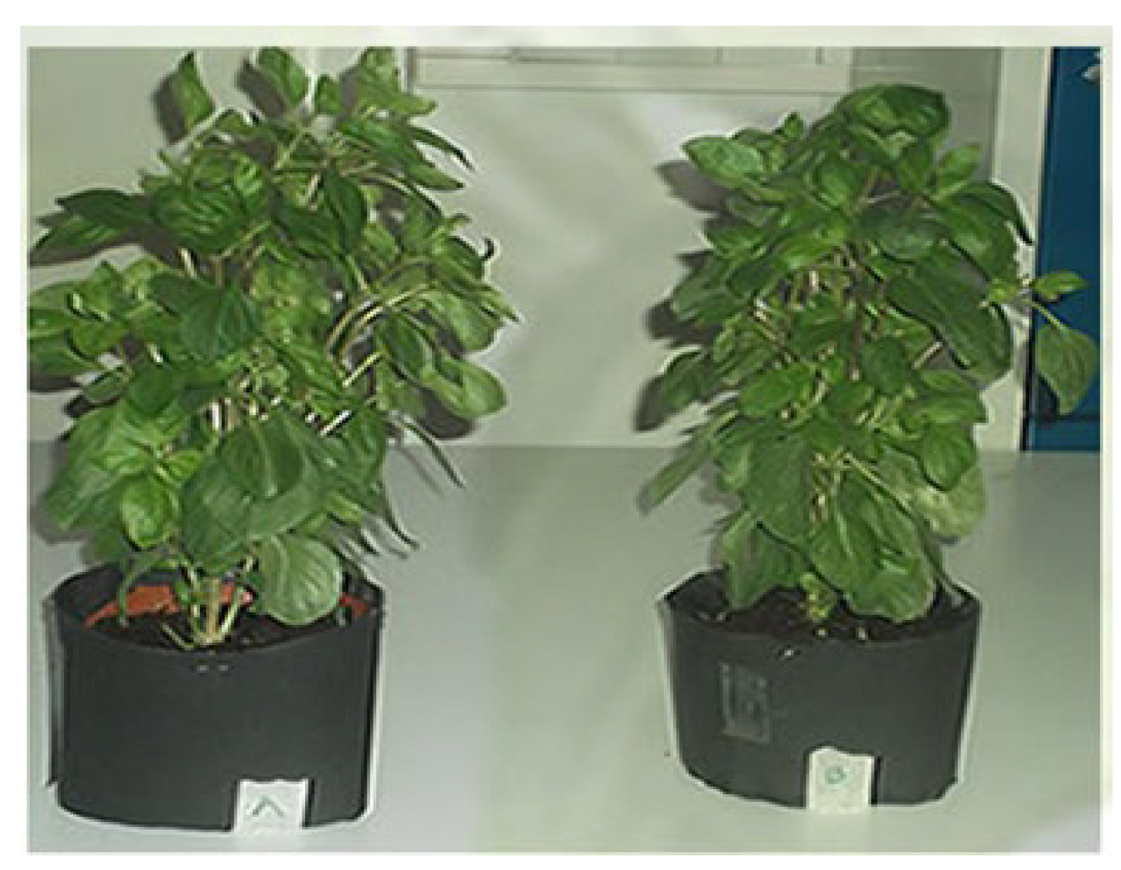
Two Basilikum Russisch plants were chosen for the purpose of this study. The Basilikum plant was chosen because of its high sensitivity to water and sunlight and could easily be stressed if there is deficiency of any of these phonological factors. These make it ideal for the study since the investigation focused on short timeframe and choosing a resistant plant variety would not be suitable. One plant was constantly watered and exposed to sunlight whilst the other was deprived of both sunlight and water for the whole duration of the study. Both plants were observed each day and images were captured for processing and analysis (Figure 2.1 and 2.4).

Figure 2. 1:Sample vegetable plants (Basilikum Russisch).

Figure 2. 1:Sample vegetable plants (Basilikum Russisch).

To allow for easy separation of the plant in the imagery and also to reduce the effects of reflection of the sun beam on the quality of the imagery, a dark background was used. The plant was positioned in the dark in the box which was lined with a matt black material during the image acquisition. The dark background station was fixed to point to maintain the same orientation for all the images taken to avoid any form of bias (Figure 2.2).

2.2. Canon Rebel 500 NDVI Camera

The canon Rebel 500 NDVI camera which captures images in the blue and near infrared band was used for image acquisition. It has a resolution of 12.2 Megapixels and has a focus of 17-35mm(www.max-max.com). This makes the cameral ideal for image for this research because of high resolution image capturing (Figure 2.3).

Figure 2. 2 and 2.3: Dark background and Canon Rebel 500 NDVI camera.

Figure 2. 2 and 2.3: Dark background and Canon Rebel 500 NDVI camera.

2.3. Image Capturing and Processing Software (Matlab)

Images of both plants were captured periodically to investigate the changes in their health. Photographs of the two plants were captured under the same conditions. A focal length of 35mm was used throughout the image acquisition and it was also ensured that the orientation of the camera with respect to the plant’s position was kept constant (Figure 2.3). The plant’s position was marked to ensure that same position is maintained in all the images captured. To minimize the influence of the reflection from the sunlight, the dark background was used. Additionally, the photographs were taken in the evening when it’s relatively dark and the influence of the sunlight is minimal (Figure 2.4).

The images captured were processed in matlab. To do this successfully, the image processing toolbox license was required. This is a matlab library which contains algorithms, functions and applications for the processing, analysis and visualization of imagery (www.mathworks.com).

2.4. Image Processing

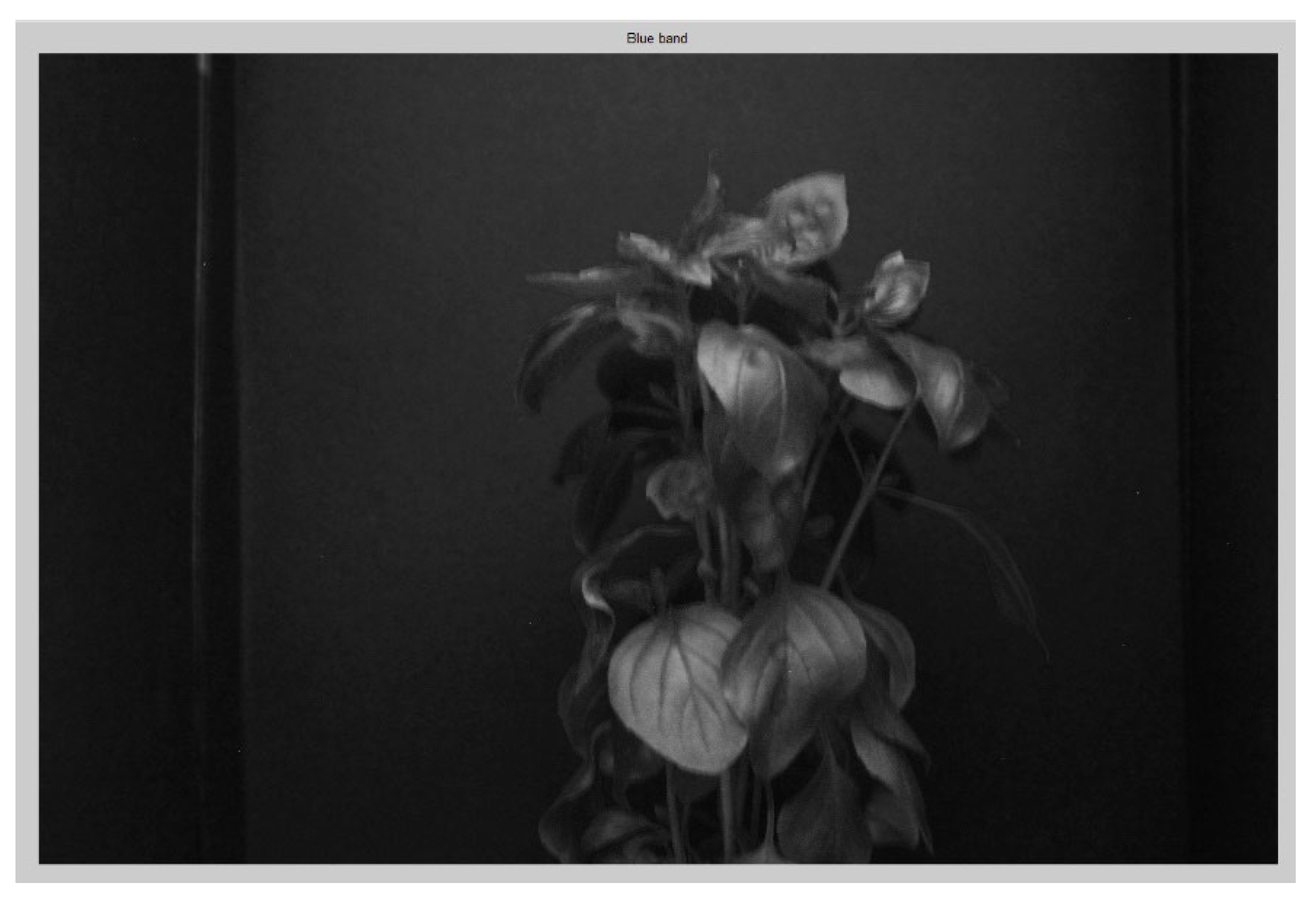
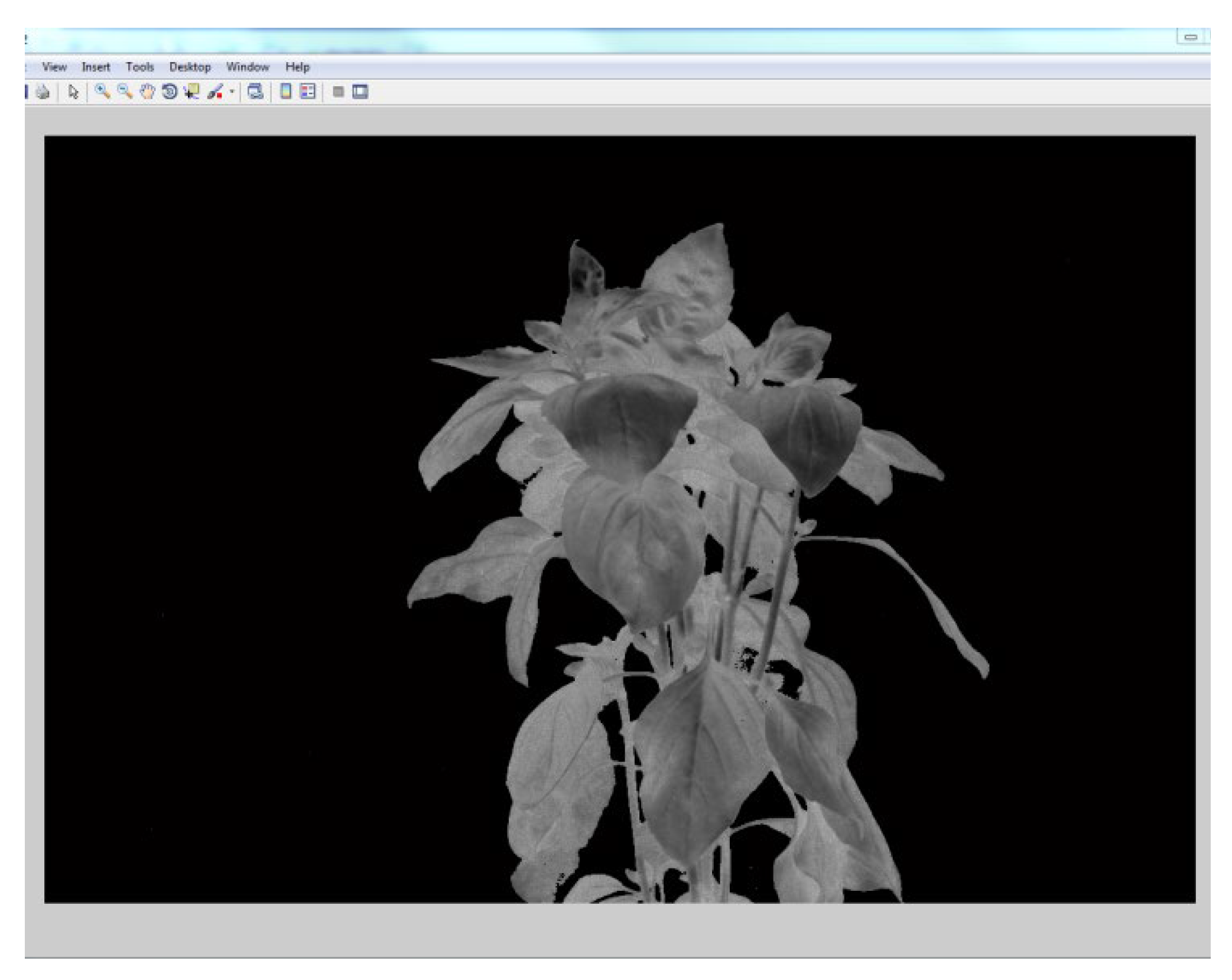
In order to achieve the main objective of the study, the plants images captured were read into matlab and processed to be separated into blue and near infrared bands. In the Canon Rebel 500 NDVI camera used for capturing, the near infrared band was calibrated as the first band, whilst the blue band is recorded as the third band. The second band constitutes noise in the imagery and hence was not used in the computation of the indices (Figure 2.5 and 2.6).

Figure 2. 4: Project Workflow.

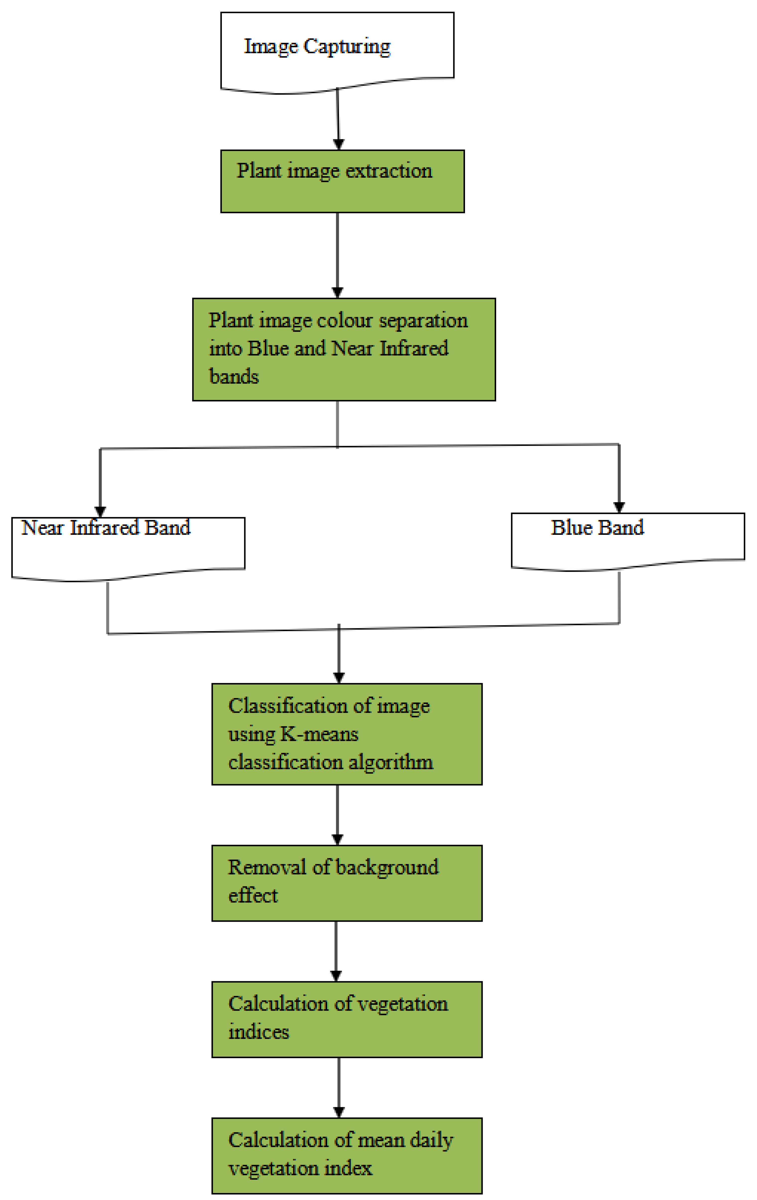
Figure 2. 4: Project Workflow.

Figure 2. 5: Near Infrared band Image.

Figure 2. 5: Near Infrared band Image.

Figure 2. 6: Blue band Image.

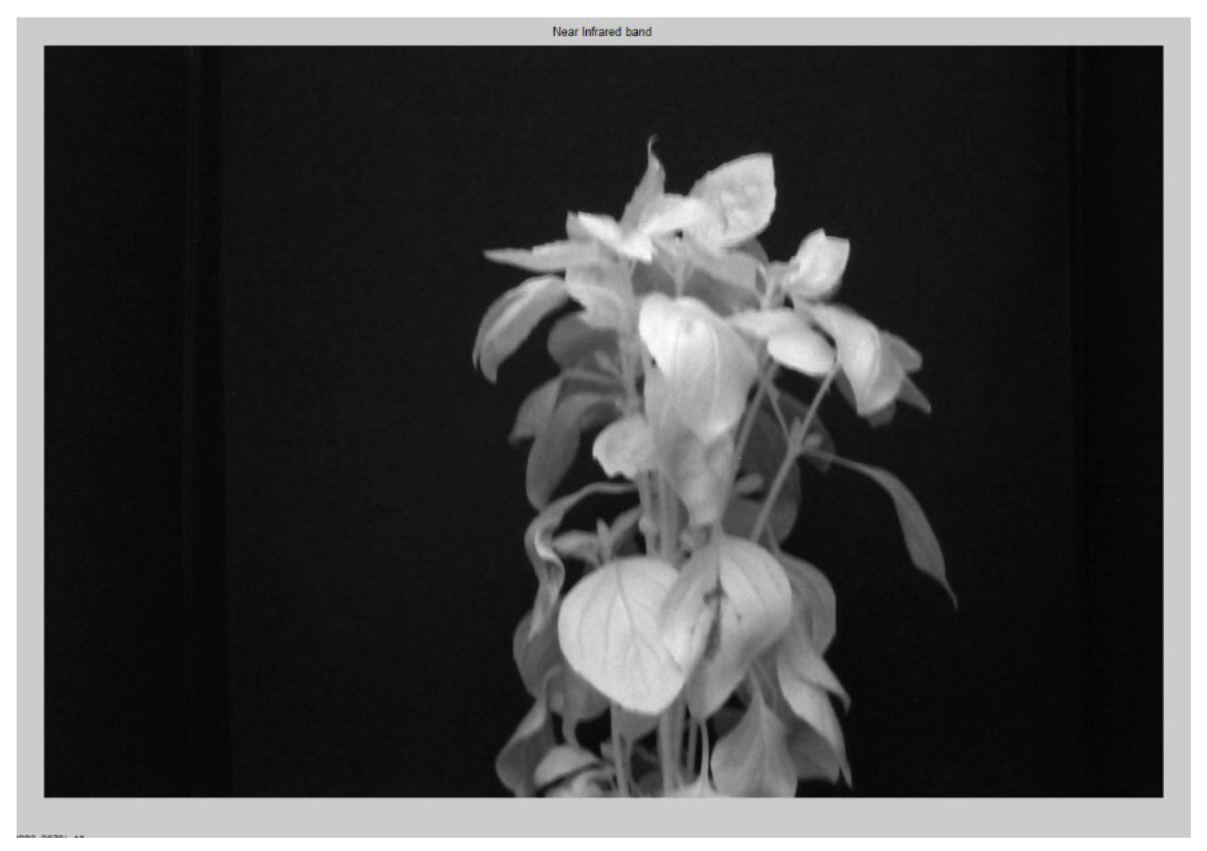
Figure 2. 6: Blue band Image.

2.5. Computation of Vegetation Indices

Vegetation information obtained remotely through sensors as images can be interpreted by differences and changes in the green leaves of plants and canopy spectral characteristics. The commonly adopted validation process is through direct or indirect correlations between vegetation indices collected and vegetation characteristics of interest observed in situ including Leave Area Index, biomass, growth and vigor assessment (Jinru and Baofeng, 2017). Healthy plants generally have a high reflectance in the near infrared band. By measuring the near infrared reflectance from a plant, the healthiness can be determined. This is achieved by computing the vegetation index of the plant. There exists various vegetation indices, however for the purpose of this research, three main vegetation indices were considered. These include: Normalized difference Vegetation index (NDVI), Infrared Percentage Vegetation Index (IPVI) and Transformed Difference Vegetation Index (TDVI). Images of the various plants under investigation were captured and then processed to compute various vegetation indices. The results were then analyzed to determine the rate of deterioration and improvement of the plants health.

This study was carried out using NDVI camera, Canon Rebel 450D which capture images in both near infrared and blue bands. However, an RGB camera EOS 350D was also adopted to capture the image to explore the possibility of calculating the Enhanced Normalised Vegetative index (ENDVI) with an additional band. Over the years, various researchers have carried out investigations into vegetative index computation and have proposed many other indices. However, NDVI remains the most popular index for monitoring plants’ health. NDVI is an index that combines visible and near-infrared bands of the electromagnetic spectrum. NDVI is normally computed as: NDVI = (NIR – Red)/ (NIR + Red), however since the NDVI camera used during this study captured images in only the NIR and Blue bands. A different formulation of the NDVI formula (NIR – Blue)/ (NIR + Blue) (www.max-max.com), was used. The various vegetation indices were computed for each of the plants for the days on which the images were captured.

Computation of NDVI

Normalise Difference Vegetation Index is calculated through a normalization process, the NDVI values ranges between 0 and 1with a sensitive response to green plants even for low vegetation covered areas (Gamon et al., 1995; Grace et al., 2007). A modification of the NDVI formula was used. Since the camera does not capture images in the red band, the following formula was used in calculating the NDVI.

$NDVI={\displaystyle \frac{(NIR-Blue)}{(NIR+Blue)}}$      1

Computation of IPVI

Another vegetative index, Infrared percentage vegetative Index (IPVI) which was developed by Crippen in 1990 was also computed for each plant and each of the observation days. The IPVI computes the percentage of the infrared reflectance of the total reflectance. This method is functionally equivalent to the NDVI, however it requires a much less computation time. IPVI values range from 0 to 1 (Jinru and Baofeng, 2017).

The formula implemented in matlab is as follows:

$IPVI={\displaystyle \frac{NIR}{NIR+BLUE}}$      2

Computation of TDVI

The Transformed difference vegetative index published by Bannari, Asalhi, and Teillet (2002) was also computed and compared with IPVI and NDVI trends.

$TDVI=1.5\mathrm{*}\lceil {\displaystyle \frac{(NIR-Blue)}{\sqrt{{NIR}^2+Blue+0.5}}}\rceil$      3

2.6. Classification of Plant Pixels

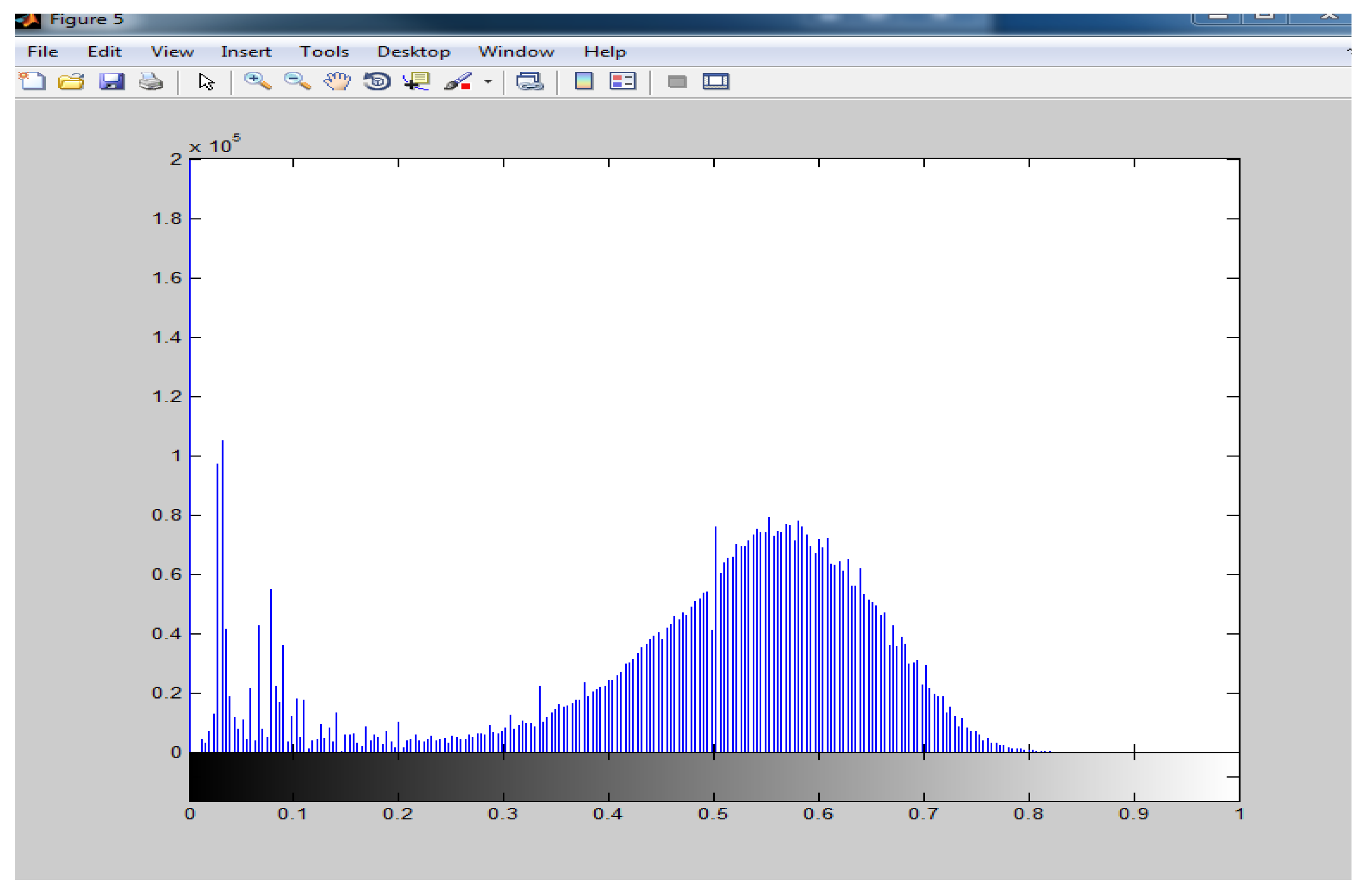
After the computation of the various indices, the next step was the classification of plant pixels. In order to identify which reflectance values represented the plant, the NDVI image histogram was used. When the histogram was plotted, it was realized that the two clusters were clearly separated. The background which formed one cluster and the plant which formed another cluster could be identified. From the histograms it was realized that there were two peaks. The beginning of the second cluster could easily be identified from the histogram. This represented the foreground (plant) (Figure 2.7).The following ranges were based on NDVI classification ranges provided by the ENDELEO project which was classified as follow: 0.2 - 0.4: Normal, 0.4-0.6: Moderately healthy, > 0.6: Most healthy (Devriendt et al., 2010).

Background Separation and Computation of the number of healthy pixels

In order to perform computation and analysis on the plant pixels alone, the plant pixels were separated from the background pixels. To monitor the health of the plant, the number of pixels with NDVI value greater than 0.6 was calculated for each image to determine whether the health of the plant was improving or deteriorating.

Figure 2. 7: Image histogram of plant.

Figure 2. 7: Image histogram of plant.

2.7. Classification of Image

The image was classified into foreground and background, K-Means classification algorithm was implemented in matlab and used .This was done by first converting the three band image into a single “LAB” color-space image. The size of the ‘LAB’ image was reshaped to the size of the original image after which two clusters were defined to represent the background and the foreground. The pixels were then labeled with the numbers representing the clusters. A binary image was produced with the labels. The binary image produced by the k-means classification was modified. The background pixels were assigned a label of ‘0’ whilst the foreground pixels were assigned a value of ‘1’ (Figure 2.8 and 2.9).This resulted in an image mask which was multiplied by the vegetative index image to eliminate the reflectance of the background pixels, hence the background was removed.

Figure 2. 8: Binary mask.

Figure 2. 8: Binary mask.

Figure 2. 9: Image with removed background.

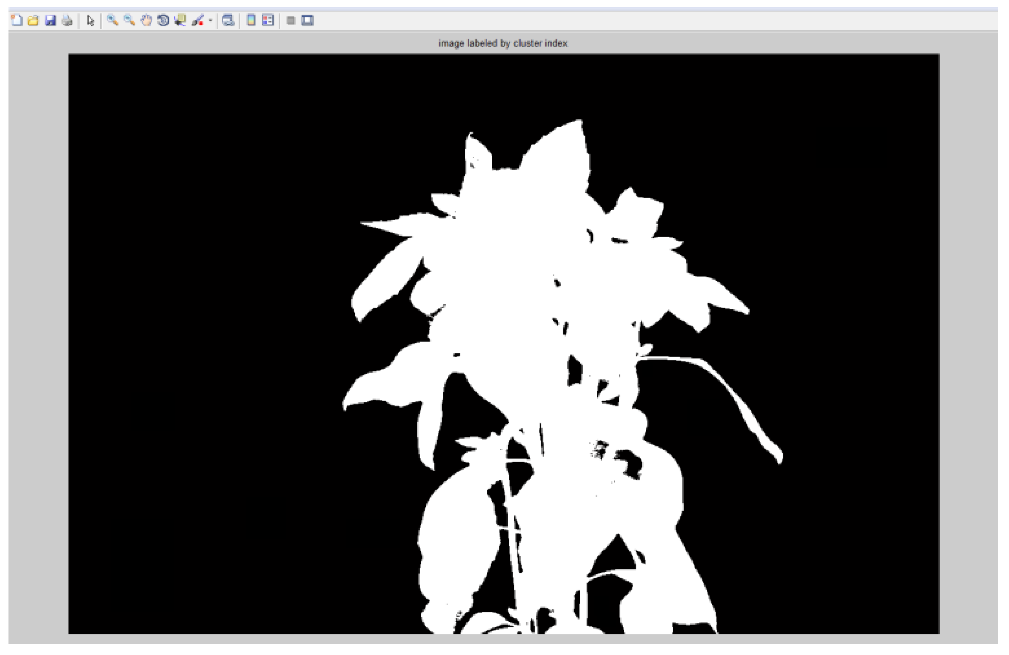
Figure 2. 9: Image with removed background.

3. Results and Discussion

3.1. Computation of Mean Daily Index

The mean daily vegetative index for each of the plants was computed by finding the mean values of the IPVI, NDVI and TVI. These values represented the Vegetation index for each day of observation. The various values were plotted against the days of observation and a trend of the observations was determined. The mean daily indices and the number of pixels of the healthy plant parts are computed and compared in the table 3.1.

Analysis from table 3.1 revealed the result of daily variation or changes in the vegetation indices of both healthy Plant referred to as Plant A and stressed plant also known as Plant B. The extent of healthiness and depreciation level of the stressed plant is measured by the number of pixels occupied by each of the plants for 28 days which is the duration of the experiment when the stressed plant (Plant B) stopped living at all. From the first day of the study in fourth of May, 2016, the aggregate of the three vegetation indices of NDVI, TDVI and IPVI of the healthy plant (Plant A) was 2086712 pixels while that of stressed plant (Plant B) occupied 397531 pixels. This indicates that both plants were at their best blossom state but plant B was healthier and thrived than it counterpart. As the time advanced from the third day of the experiment, plant A improved in its health status to occupied the total pixels of 2453313 while that of plant B commenced its depreciation to 212499 pixels. This marked the beginning and first stage of the observation of the exposure of wetting plant A with adequate water at appropriate time and exposed same to sunlight for access to chlorophyll while plant B was deprived of these essential resources (Figure 3.7).

The next stage in the analysis was the beginning decline of the stressed plant (plant B) and the gradual increased in the healthiness status of Plant A (healthy plant). That is the stressed plant depreciated from its peak at 399021 pixels on the second day (5/5/2016) of the experiment to 0 pixel when the plant became completely dead on the 27^th days of the experiment (10/6/2016). The health condition of the Plant B (unhealthy plant) depreciated due to the condition the plant was subjected to such as water and sunlight deprivation. This shows that, Russiches Basilicum plant cannot survive outside water and sunlight for 27 days. The healthy plant (plant A) on the other hand, the health status of this plant appreciated tremendously from the 2^nd day (5/5/2016) from 2086712 pixels to its peak at 4913780 pixels on the 11/6/2016 which was the last day of the experiment (Figure 3.8).

Table 3. 1: Daily NDVI,TDVI and IPVI indices for healthy and stressed plants and daily monitored health status pixels calculation.

Date	Plant A NDVI	Plant A TDVI	Plant A IPVI	Health condition pixel no in A	Plant B NDVI	Plant B TDVI	Plant B IPVI	Health condition pixel no in B
4-5-2016	0.5573	1.0679	0.7765	2086712	0.5082	1.0023	0.7541	397531
5-5-2016	0.5573	1.0679	0.7663	2086712	0.505	0.9982	0.76	399021
6-5-2016	0.5475	1.0520	0.7804	2453313	0.4848	0.9703	0.7472	212499
7-5-2016	0.5381	1.0358	0.7667	2605717	0.4902	0.9777	0.749	18003
8-5-2016	0.5363	1.0369	0.7608	2517104	0.4969	0.9877	0.7546	259418
9-5-2016	0.5404	1.0427	0.7710	2719444	0.4739	0.9527	0.7234	151183
11-5-2016	0.5366	1.0525	0.7673	2604557	0.4778	0.961	0.742	160966
12-5-2016	0.554	1.0579	0.7820	3129870	0.4809	0.9647	0.7462	186586
13-5-2016	0.5324	1.0298	0.7663	2908670	0.4873	0.972	0.7507	235232
15-5-2016	0.5458	1.0460	0.7725	3500470	0.3947	0.8333	0.7055	32345
16-5-2016	0.5301	1.0263	0.7640	3106565	0.394	0.8329	0.4203	30760
18-5-2016	0.5521	1.0567	0.7762	3378703	0.3267	0.7271	0.6619	2304
19-5-2016	0.546	1.0478	0.7726	3451196	0.3122	0.7023	0.4114	593
20-5-2016	0.5494	1.0515	0.7743	3767465	0.241	0.571	0.3738	469
22-5-2016	0.5626	1.0151	0.5682	5373199	0.2218	0.5	0.38	404
27-5-2016	0.5856	1.0864	0.7977	5512211	0.22	0.4912	0.4086	21
28-5-2016	0.5538	1.0605	0.7754	3837543	0.2129	0.491	0.3602	14
29-5-2016	0.5398	1.0412	0.7666	3325143	0.2449	0.49	0.3876	12
30-5-2016	0.523	1.0201	0.7560	2606545	0.2002	0.4883	0.355	9
1-6-2016	0.5366	1.0364	0.7668	3547954	0.2657	0.6149	0.3853	5
2-6-2016	0.5582	1.0730	0.7736	3757092	0.2199	0.5255	0.3776	3
3-6-2016	0.5663	1.0760	0.7858	4527577	0.2061	0.5005	0.38	3
5-6-2016	0.5696	1.0766	0.7621	4579065	0.1859	0.4576	0.3422	2
6-6-2016	0.5643	1.0729	0.7646	4749141	0.183	0.448	0.3575	2
8-6-2016	0.5647	1.0777	0.7691	4912710	0.1825	0.432	0.3978	1
9-6-2016	0.5648	1.0844	0.7577	4912820	0.182	0.41	0.3543	1
10-6-2016	0.566	0.0858	0.7562	4913271	0.18	0.379	0.4287	0
11-6-2016	0.567	1.0868	0.7581	4913780	0.177	0.347	0.3923	0

Table 3. 1: Daily NDVI,TDVI and IPVI indices for healthy and stressed plants and daily monitored health status pixels calculation.

Date	Plant A NDVI	Plant A TDVI	Plant A IPVI	Health condition pixel no in A	Plant B NDVI	Plant B TDVI	Plant B IPVI	Health condition pixel no in B
4-5-2016	0.5573	1.0679	0.7765	2086712	0.5082	1.0023	0.7541	397531
5-5-2016	0.5573	1.0679	0.7663	2086712	0.505	0.9982	0.76	399021
6-5-2016	0.5475	1.0520	0.7804	2453313	0.4848	0.9703	0.7472	212499
7-5-2016	0.5381	1.0358	0.7667	2605717	0.4902	0.9777	0.749	18003
8-5-2016	0.5363	1.0369	0.7608	2517104	0.4969	0.9877	0.7546	259418
9-5-2016	0.5404	1.0427	0.7710	2719444	0.4739	0.9527	0.7234	151183
11-5-2016	0.5366	1.0525	0.7673	2604557	0.4778	0.961	0.742	160966
12-5-2016	0.554	1.0579	0.7820	3129870	0.4809	0.9647	0.7462	186586
13-5-2016	0.5324	1.0298	0.7663	2908670	0.4873	0.972	0.7507	235232
15-5-2016	0.5458	1.0460	0.7725	3500470	0.3947	0.8333	0.7055	32345
16-5-2016	0.5301	1.0263	0.7640	3106565	0.394	0.8329	0.4203	30760
18-5-2016	0.5521	1.0567	0.7762	3378703	0.3267	0.7271	0.6619	2304
19-5-2016	0.546	1.0478	0.7726	3451196	0.3122	0.7023	0.4114	593
20-5-2016	0.5494	1.0515	0.7743	3767465	0.241	0.571	0.3738	469
22-5-2016	0.5626	1.0151	0.5682	5373199	0.2218	0.5	0.38	404
27-5-2016	0.5856	1.0864	0.7977	5512211	0.22	0.4912	0.4086	21
28-5-2016	0.5538	1.0605	0.7754	3837543	0.2129	0.491	0.3602	14
29-5-2016	0.5398	1.0412	0.7666	3325143	0.2449	0.49	0.3876	12
30-5-2016	0.523	1.0201	0.7560	2606545	0.2002	0.4883	0.355	9
1-6-2016	0.5366	1.0364	0.7668	3547954	0.2657	0.6149	0.3853	5
2-6-2016	0.5582	1.0730	0.7736	3757092	0.2199	0.5255	0.3776	3
3-6-2016	0.5663	1.0760	0.7858	4527577	0.2061	0.5005	0.38	3
5-6-2016	0.5696	1.0766	0.7621	4579065	0.1859	0.4576	0.3422	2
6-6-2016	0.5643	1.0729	0.7646	4749141	0.183	0.448	0.3575	2
8-6-2016	0.5647	1.0777	0.7691	4912710	0.1825	0.432	0.3978	1
9-6-2016	0.5648	1.0844	0.7577	4912820	0.182	0.41	0.3543	1
10-6-2016	0.566	0.0858	0.7562	4913271	0.18	0.379	0.4287	0
11-6-2016	0.567	1.0868	0.7581	4913780	0.177	0.347	0.3923	0

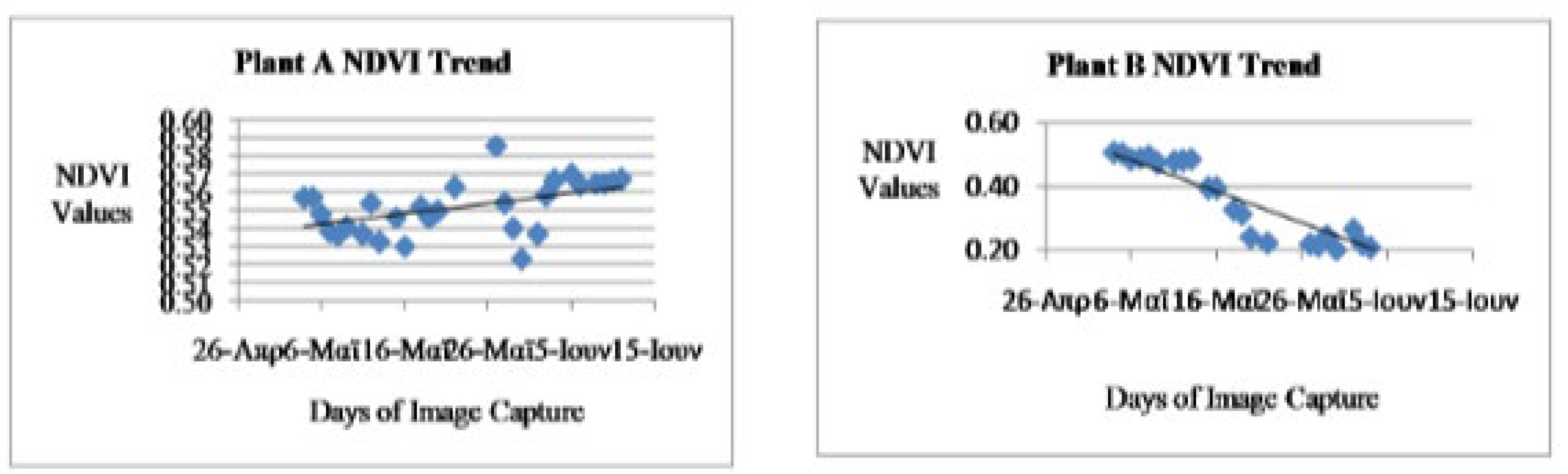
The NDVI analysis trend of the result as shown in the best fit line of Figures 3.1 and 3.2 revealed gradual increased in the NDVI values of the healthy plant (Plant A) and vice versa in the NDVI values of the stressed plant (Plant B). I t should be noted that NDVI measure the greenness level of plants which its value ranges from 0 – 1 that is from dead or completely non-green status of the plant to full green status of the plant. This is however a function of water, chlorophyll and other phonological factors. The NDVI values of Plant A initially depreciated from the first day of the experiment of 0.5573 to 0.523 on 30-5-2016 which was the 19^th days of the study which could be due to the deficiency of certain phonological factors. Later, the NDVI values improved to the highest point at 0.5856 and lastly 0.567 on the 28^th days of the study which was the last day of the study (Figure 3.1). The reason for the variation as depreciation instead of appreciation as expected in the first phase could be as a result of changes in the quantity of phonological factors such as air, sunlight, water etc availability was below the minimum required quantity by the plant and other way round for the well pronounced increase in the value even as the time advances. On the other hand, the NDVI values of the stressed plant (Plant B) revealed gradual depreciation from the first day with 0.5082 to 0.177 on the last day of the experiments when the plant became dead completely. The reason for the 0.177 NDVI value on the last day was due to the little greenness sensed in the withered plant (Figure 3.2).

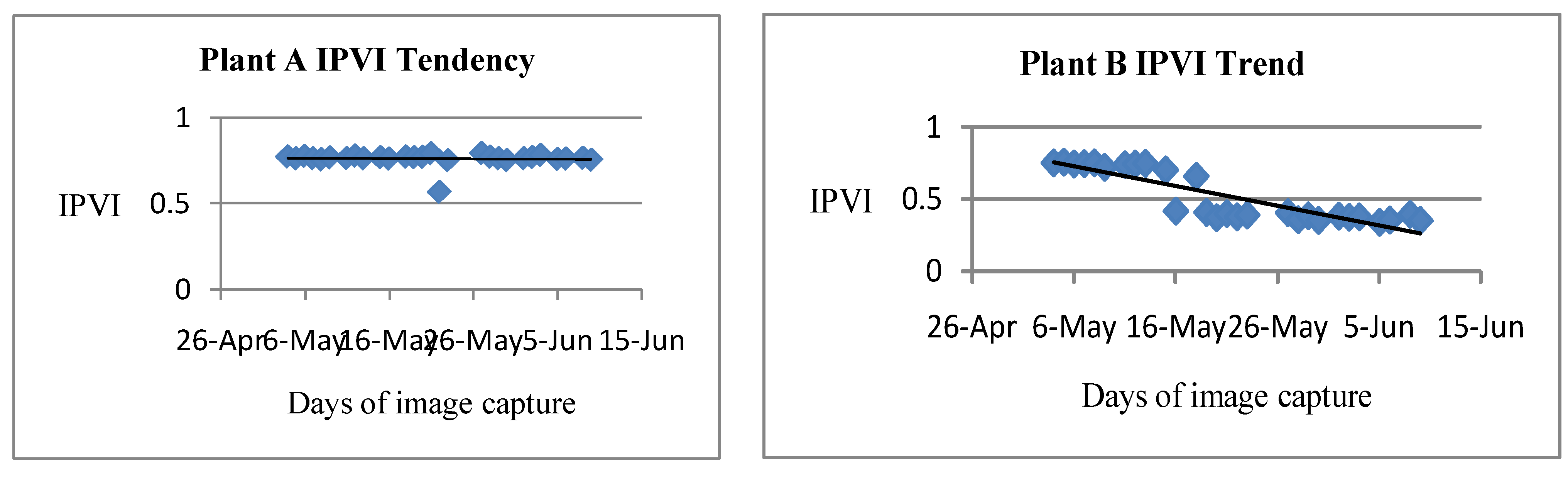
Vegetation analysis of the IPVI trend result as revealed in both Figure 3.3 and Figure 3.4 shows different level of changes in term of increase and decrease in the IPVI values of both healthy (Plant A) and stressed plant (Plant B). The IPVI vegetation value of healthy plant (Plant A) improved from 0.7765 on the first day of the experiment to 0.7804 on the 3^rd day and later depreciated to the lowest value at 0.5682 on the 22^nd May 2016 which was day 15^th of the experiment. The thriving status of Plant A improved to its peak at 0.7977 IPVI value and later reduced in value to 0.7581 on the last day of the experiment. The stressed plant (Plant B) on the other hand initially depreciated from the blossom state of the plant on the first day (4/5/2016) with the IPVI value of 0.7541 to 0.4203 on the 16^th of June 2016 and later appreciated to 0.6619 but at the end depreciated to the least value of 0.3923 on the last day. The rate of appreciation and diminishing level of both plants of study could be traced to different proportions of phonological factors available at different dates of observation such as above, below or exact proportions required for the growth of Russiches Basilicum plant.

Analysis of the TDVI vegetation index computation as presented in Figure 3.5 and Figure 3.6 indicated various degrees of changes in the health status of the observed plants in the study. The healthy plant (Plant A) health status as computed using TDVI revealed gradual appreciation from 1.0679 and later declined to its lowest state at 1.0151 on the 15^th days of the experiment. The TDVI measure of the healthy plant improved to the highest point of 1.0868 on the last day of the study. The stressed or unhealthy plant on the other hand TDVI measure revealed depreciation in the health status from 1.0023 in the first day to 0.4883 on the 16^th day but improved to 0.6149 on the 17^th day of the study. At the end of this index measure, the Plant B depreciated to 0.347 on the last day of the experiment (Figure 3.6). Measuring the vegetation status of the study plants was affected by the available quantity of series of phonological factors during the period of the study.

NDVI Trend

Figure 3. 1: NDVI tendency for the healthy plant A Figure 3.2: TDVI trend for unhealthy plant B.

Figure 3. 1: NDVI tendency for the healthy plant A Figure 3.2: TDVI trend for unhealthy plant B.

IPVI Trend

Figure 3. 3: IPVI trend of healthy plant A Figure 3.4: IPVI trend of unhealthy plant.

Figure 3. 3: IPVI trend of healthy plant A Figure 3.4: IPVI trend of unhealthy plant.

TDVI Trend

Figure 3. 5: TDVI trend of the healthy plant A Figure 3.6: TDVI trend of unhealthy plant B .

Figure 3. 5: TDVI trend of the healthy plant A Figure 3.6: TDVI trend of unhealthy plant B .

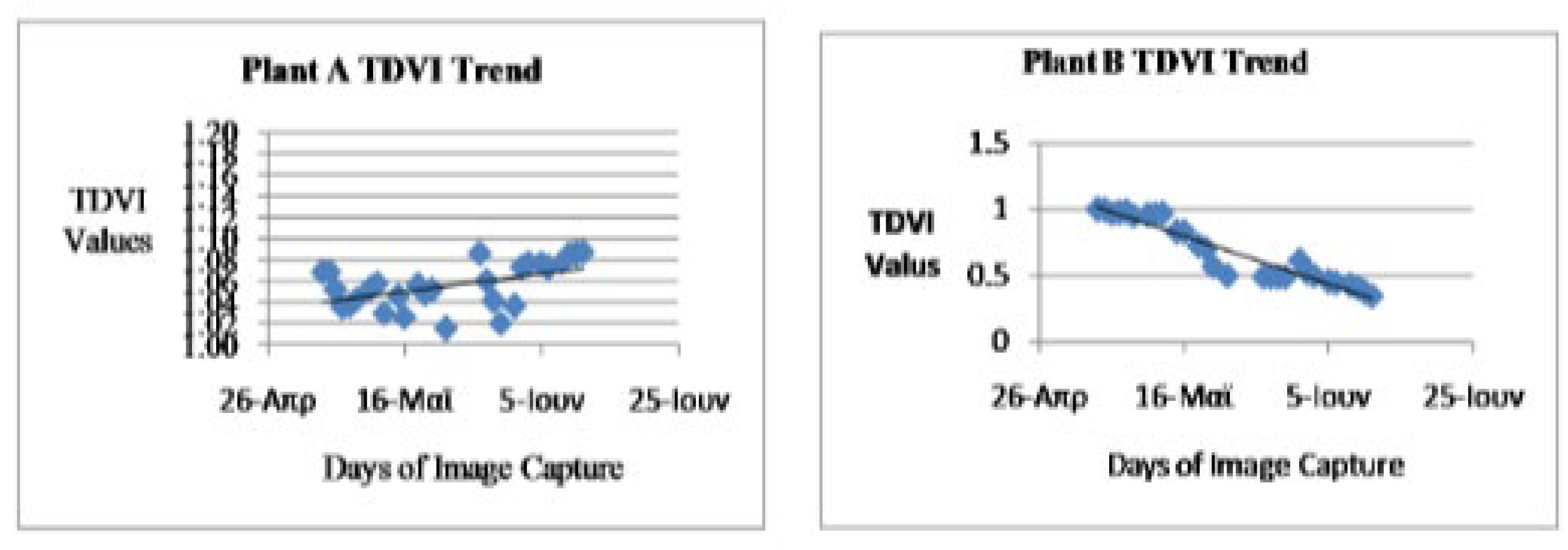
Figure 3. 7: Trend of pixels of healthy parts of plant A Figure 3.8: Trend of pixels of unhealthy parts of plant B.

Figure 3. 7: Trend of pixels of healthy parts of plant A Figure 3.8: Trend of pixels of unhealthy parts of plant B.

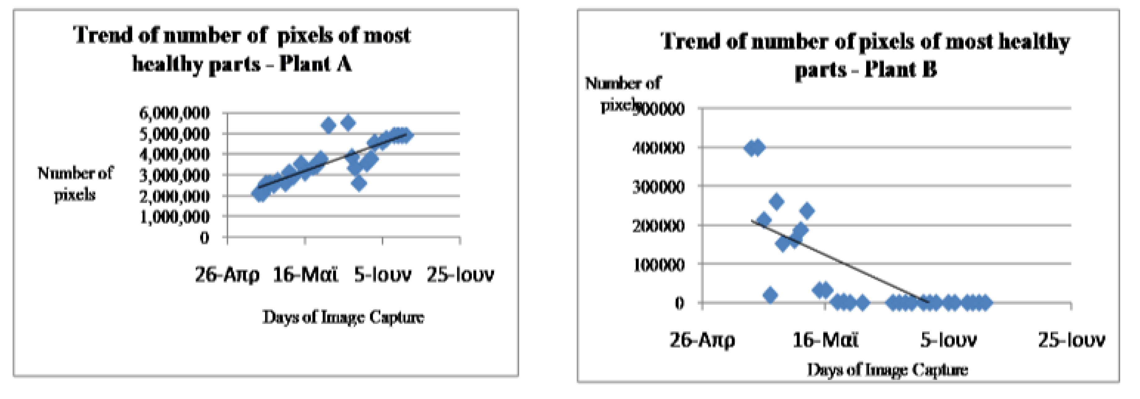
The graphs show the trend of the NDVI, TDVI and IPVI indices during the days of observation, for both plant A and plant B. Plant A is considered as healthy because it was treated under favorable conditions. It was watered daily and kept in the sun. For this reason, plant A was able to conduct daily the Photosynthesis process with high metabolic rhythm which resulted in its high chlorophyll content. In lieu of that, there is a general increase in the number of healthy pixels as shown in the table 1 and the Near Infrared reflectance in this plant during the period of this research. This can be seen in the trend of the indices. However an inspection of the trend of the indices for plant B showed that there was a decrease in the number of healthy pixels and the various indices. This is as a result of the fact that plant B was rarely watered and not exposed to enough sunlight. This resulted in the decrease of chlorophyll content of the plant and near infrared reflectance. It was realized that during some of the days, there was a decrease in the indices of plant A, when an increase was expected. This can be attributed to the biological characteristics of the species of the vegetable plant (Basillicum) used and also changes in weather conditions. The plant is highly sensitive to changes in phonological factors such as water and sunlight. During foggy days, since there is not enough sunlight available, a drop in the indices was generally experienced (Figure 3.7 and 3.8).

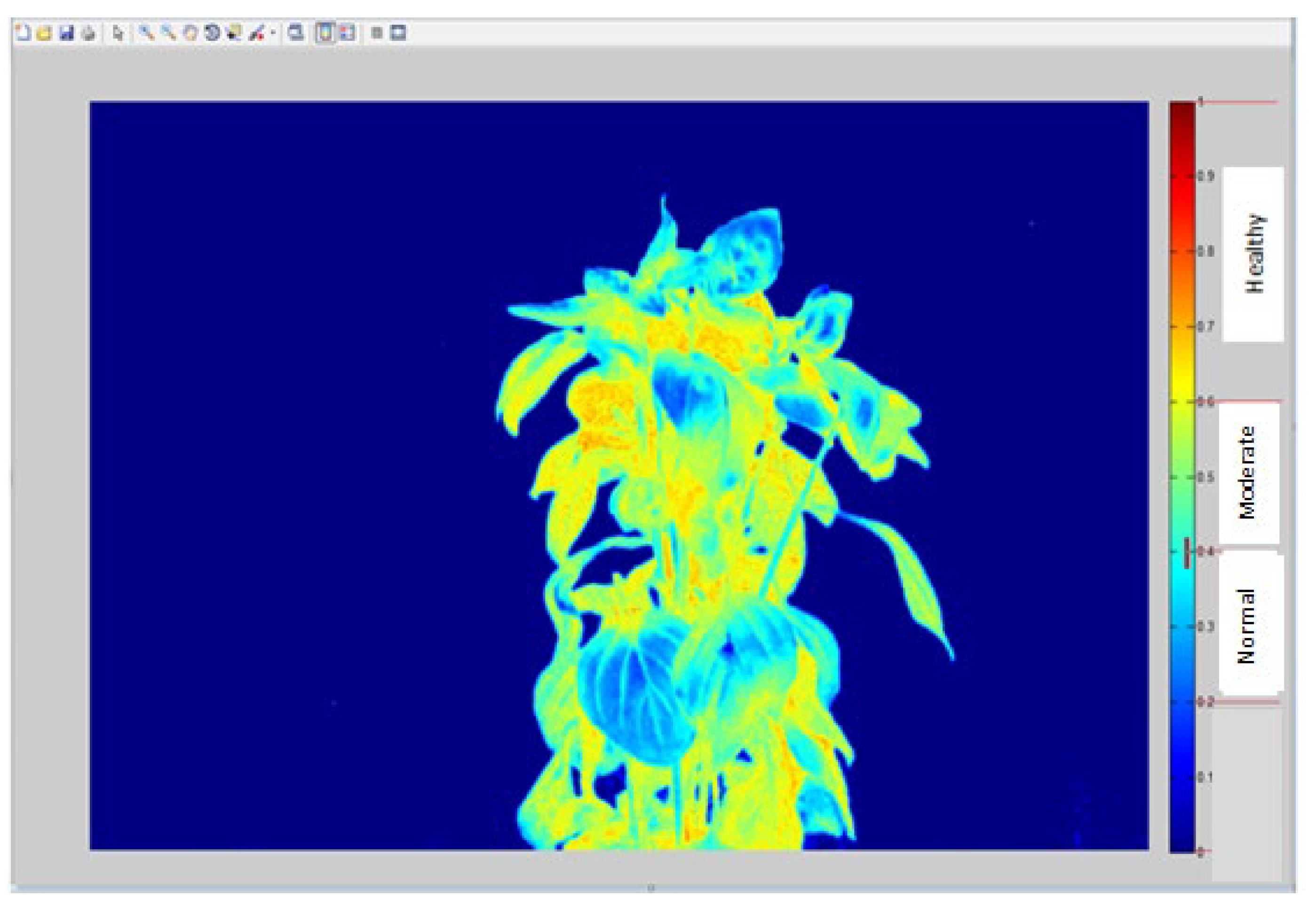
The NDVI plant image pixels classification as shown in Figure 3.9 revealed the classification of image into three classes of normal, moderate and healthy portion of the plant. The normal part of the plant as processed by Matlab include the region between 0 – 0.4, the region range between 0.4 – 0.7 is classified as moderate while spectrum range between 0.7 – 1.0 is known as healthy portion of the plant. Results from NDVI image analysis revealed that the healthy plant’s status reflected moderately healthy situation with its result ranges from 0.52 – 0.7 and that of stressed plant is classified as normal moderate with recorded region of 0.18 – 0.51. The reason why the healthy plant was not fully healthy according to the pixel classification could be due to the fact this was a controlled experiment inside the room except for the duration that plant was taken out daily to receive sunlight and air while these essential phonological factors were deficient when the plant was returned back to its confinement area and vice versa for the stressed plant (Figure 3.9).

Figure 3. 9: NDVI image of plant showing the various classified pixels.

Figure 3. 9: NDVI image of plant showing the various classified pixels.

4. Conclusions

The vegetation stress map is a very effective measure in determining the level of healthiness in plants and indeed goes a long way in determining the yield of the plant as carried out in this project. The outcome of this project reveals the sensitivity of plants (vegetable) to water and sunlight, which are the major factors for photosynthesis in which their inadequate supply will lead to poor health condition of plants and result in drastic reduction in yield. If this is detected earlier in plants, preventive measure can salvage the situation as in the case of short-term, otherwise it could lead to total death of the plants. The different vegetation indices (NDVI, TDVI, and IPVI) employed during the study proved appropriate to evaluate and compare results from the project. All the three indices showed the same trend for both plants although formula for the indices take into account different considerations. Computation of the number of healthy plant pixels also confirmed the trend of health of both plants as established by the use of the vegetative indices. This experiment could however form a very good basis for agricultural crop yield research in all climatic regions. The Tli 450D Cannon Rebel NDVI camera used during this experiment was very effective because plants absorbed more radiations in the blue band and reflected more in the NIR band hence an analysis of reflectance from both bands was used to monitor the condition of the plan.

References

- Abdullah, H., R. Darvishzadeh, A. K. Skidmore, T. A. Groen,and M. Heurich. 2018. European spruce bark beetle (Ipstypographus, L.) green attack affects foliar reflectance andbiochemical properties. Int. J. Appl. Earth Obs. Geoinf. 64, 199–209.
- Ali, A. M., R. Darvishzadeh, A. K. Skidmore, I. V. Duren, U. Heiden, and M. Heurich. 2016. Estimating leaf functional traits by inversion of PROSPECT: assessing leaf dry matter content and specific leaf area in mixed mountainous forest. Int. J. Appl. Earth Obs. Geoinf. 45, 66–76.
- Bannari, A., Morin, D., Huete, A.R. and Bonn, F. (1995) A review of vegetation indices. Remote Sensing Reviews, vol. 13, p. 95-120.
- Bannari, A., H. Asalhi, and P. Teillet. "Transformed Difference Vegetation Index (TDVI) for Vegetation Cover Mapping" In Proceedings of the Geoscience and Remote Sensing Symposium, IGARSS '02, IEEE International, Volume 5 (2002).
- Carpenter GA, Gopal S, Macomber S, Martens S, Woodcock E (1999) A neural network method for mixture estimation for vegetation mapping. Remote Sens Environ 70:138–152.
- Chen, Z., Sun, S., Wang, Y., Wang, Q., Zhang, X., 2020. Temporal convolution-networkbased models for modeling maize evapotranspiration under mulched drip irrigation. Comput. Electron. Agric. 169, 105206.
- Crippen, R. "Calculating the Vegetation Index Faster." Remote Sensing of Environment 34 (1990): 71-73.
- Dada, E. and Dada, V.T. (2020), Sptatio-Temporal Analysis of Land Use and Land Cover Change in the Cocoa Belt of Ondo State, Southwestern Nigeria.Inderscience Journal Inderscience Journal of Agriculture, Innovation, Technology and Globalisation. DOI: 10.1504/IJAITG.2019.10024542.
- Dada, E. and Hahn, M. (2020), Application of satellite remote sensing to observe and analyse temporal changes of cocoa plantation in Ondo State, Nigeria. Springer Geojournal Spatially Integrated Social and Humanity. DOI: 10.1007/s1070808-020-10243-y.
- Dada, E., Orimoogunje, O.O.I and Eludoyin, O.A. (2023), Optical Remotely Sensed Data for Mapping Variations in Cashew Plantation Distribution and Associated Land Uses in Ogbomoso, Nigeria Southwest. Springer Geojournal Spatially Integrated Social and Humanity. Doi,org/10.100708-023-10861-2.
- Darvishzadeh, R., C. Atzberger, A. Skidmore, and A. Abkar. 2009. Leaf Area Index derivation from hyperspectral vegetation indicesand the red edge position. Int. J. Remote Sens. 30, 6199–6218.
- Devriendt, F., Westra, T., Dewwf, R., Delrue, J., Swinnen, E., Bydekerke, L., SItunna, C. and Lambrechts, C. (2010), Remote sensing based service to monitor vegetation dynamics in Kenya; The ENDELEO tool. Earth observation,1-20.
- Filchev, L. 2012. An assessment of european spruce bark beetle infestation using WorldView-2 Satellite data, Proceedings of 1st European SCGIS Conference with International Participation―Best Practices: Application of GIS Technologies for Conservation of Natural and Cultural Heritage Sites (SCGIS-Bulgaria, Sofia), Sofia, Bulgaria, pp. 21–23.
- Franklin, S., M. Wulder, R. Skakun, and A. Carroll. 2003. Mountain pine beetle red-attack forest damage classification using stratified Landsat TM data in British Columbia Photogrammetric Canada. Eng. Remote Sens. 69, 283–288.
- Gamon, J. A., Field, C. B. and Goulden M. L.(1995). “Relationships between NDVI, canopy structure, and photosynthesis in three Californian vegetation types,” Ecological Applications, 5(1)28–41, 1995.
- Gitelson, A. A., G. P. Keydan, and M. N. Merzlyak (2006). Three-band model for noninvasive estimation ofchlorophyll, carotenoids, and anthocyanin contents in higher plant leaves. Geophys. Res. Lett. 33, L11402. https://doi.org/10.1029/2006gl026457.
- Grace, J., Nichol, C., Disney, M., Lewis, P., Quaife, T and Bowyer, P. (2007). “Can we measure terrestrial photosynthesis from space directly, using spectral reflectance and fluorescence?” Global Change Biology, 13 (7) 1484–1497.
- Hava_sov_a, M., T. Bucha, J. Feren_c_ık, and R. Jaku_s. 2015. Applicability of a vegetation indices-based method to mapbark beetle outbreaks in the High Tatra Mountains. Ann. For. Res. 58, 295–310.
- He C, Zhang Q, Li Y (2005) Zoning grassland protection area using remote sensing and cellular automata modeling—acase study in Xilingol steppe grassland in northern China. J Arid Environ 63:814–826.
- Hendry, G. A., J. D. Houghton, and S. B. Brown. 1987. The degradation of chlorophyll—a biological enigma. NewPhytol. 107, 255–302.
- Huete A., Didan K., Shimabukuro Y.E., Batana P., Saleska, Hutyra L., et al. 2002), Amazon rainforests green-up with sunlight in dry season. Geophysical Research Letters, 33, P. L06405.
- Immitzer, M., and C. Atzberger (2014). Early detection of bark beetle infestation in norway spruce (Picea abies, L.) usingWorldView-2 Data<BR> Fr€uhzeitige Erkennung von Borkenk€a ferbefall an Fichten mittels WorldView-2 Satellitendaten. Photogrammetrie - Fernerkundung -Geoinformation 2014, 351–367.
- Jackson, R. D., and A. R. Huete. 1991. Interpreting vegetation indices. Prev. Vet. Med. 11, 185–200.
- Jinru, X., Baofeng, S. (2017) Significant remote sensing vegetation indices: A review of development and applications. Journal of sensors,10:1-17, doi.org/10.115/2017/1353691.
- Karnieli,A., Agam, N. and Pinker, R.T. (2010). “Use of NDVI and land surface temperature for drought assessment: merits and limitations,” Journal of Climate, 23(3) 618–633.
- Lausch, A., M. Heurich, and L. Fahse. 2013a. Spatio-temporal infestation patterns of Ips typographus (L.) in the BavarianForest National Park. Germany. Ecol. Ind. 31, 73–81.
- Li, D., Gu, X., Yong, P., Chen, B., Liu, L., 2018. Estimation of forest aboveground biomass and leaf area index based on digital aerial photograph data in Northeast China. Forests 9, 275.
- Liang, W., Hcab, C., Jza, B., Jza, B., Yza, B., Dsa, B., Xda, B., Li, Z., Hwa, B., Yla, B., 2020. Grain yield prediction of rice using multi-temporal UAV-based RGB and multispectral images and model transfer – a case study of small farmlands in the South of China. Agric. For. Meteorol. 291.
- Meddens, A. J. H., J. A. Hicke, L. A. Vierling, and A. T. Hudak. 2013. Evaluating methods to detect bark beetlecausedtree mortality using single-date and multi-date Landsat imagery. Remote Sens. Environ. 132, 49–58.
- Mutanga O, Skidmore AK (2004) Narrow band vegetation indices solve the saturation problem in biomass estimation.Int J Remote Sens 25:3999–4014.
- www. maxmax.com.
- NASA Earth Observation: Measuring Vegetation Indices, John Weier and David Herring. http://earthobservatory.nasa.gov/Features/MeasuringVegetation/. Accessed several times.
- www.endeleo.vgt.vito.be/dataproducts.html.
- Niemann, K. O., and F. Visintini. 2005. Assessment of potential for remote sensing detection of bark beetleinfestedareas during green attack: a literature review. Natural Resources Canada. Canadian Forest Service, pp. 1–14.
- Nielsen, D.C., Miceli-Garcia, J.J., Lyon, D.J., 2012. Canopy cover and leaf area index relationships for wheat, triticale, and corn. Agron. J. 104, 1569–1573.
- Ortiz, S., J. Breidenbach, and G. K€andler. 2013. Early detection of bark beetle green attack using TerraSAR-X and RapidEyedata. Remote Sens. 5, 1912–1931.
- Pereira, L.S., Paredes, P., Melton, F., Johnson, L., Wang, T., Lopez-Urrea, ´ R., Cancela, J. J., Allen, R.G., 2020. Prediction of crop coefficients from fraction of ground cover and height. Background and validation using ground and remote sensing data. Agric. Water Manag. 241, 106197-106197.
- Poças, ˆ I., Calera, A., Campos, I., Cunha, M., 2020. Remote sensing for estimating and mapping single and basal crop coefficientes: a review on spectral vegetation indices approaches. Agric. Water Manag. 233, 106081-106081.
- Qiao, K., Zhu, W., Xie, Z., Li, P., 2019. Estimating the seasonal dynamics of the leaf area index using piecewise LAI-VI relationships based on phenophases. Remote Sens. 11.
- Rischbeck, P., Elsayed, S., Mistele, B., Barmeier, G., Heil, K., Schmidhalter, U., 2016. Data fusion of spectral, thermal and canopy height parameters for improved yield prediction of drought stressed spring barley. Eur. J. Agron. 78, 44–59.
- Rullan-Silva, C. D., A. E. Olthoff, J. A. Delgado de la Mata, and J. A. Pajares-Alonso. 2013. Remote monitoring of forestinsect defoliation – a review. For. Syst. 22, 377.
- Seo, B., Lee, J., Lee, K.D., Hong, S., Kang, S., 2019. Improving remotely-sensed crop monitoring by NDVI-based crop phenology estimators for corn and soybeans in Iowa and Illinois, USA. Field Crops Res. 238, 113–128.
- Shao, G., Han, W., Zhang, H., Zhang, L., Wang, Y. and Zhang, Y., 2023. Prediction of maize crop coefficient from UAV multisensory remote sensing using machine learning methods. Agric. Water Manag. 276, 108064.
- Shao, G., Han, W., Zhang, H., Liu, S., Wang, Y., Zhang, L., Cui, X., 2021. Mapping maize crop coefficient Kc using random forest algorithm based on leaf area index and UAVbased multispectral vegetation indices. Agric. Water Manag. 252, 106906.
- Seidl, R., M.-J. Schelhaas, W. Rammer, and P. J. Verkerk. 2014. Increasing forest disturbances in Europe and theirimpact on carbon storage. Nat. Clim. Change 4, 806–810.
- Wulder, M. A., J. C. White, A. L. Carroll, and N. C. Coops. 2009. Challenges for the operational detection of mountainpine beetle green attack with remote sensing. For. Chron. 85, 32–38.
Disclaimer/Publisher’s Note: The statements, opinions and data contained in all publications are solely those of the individual author(s) and contributor(s) and not of MDPI and/or the editor(s). MDPI and/or the editor(s) disclaim responsibility for any injury to people or property resulting from any ideas, methods, instructions or products referred to in the content. |
© 2024 by the authors. Licensee MDPI, Basel, Switzerland. This article is an open access article distributed under the terms and conditions of the Creative Commons Attribution (CC BY) license (http://creativecommons.org/licenses/by/4.0/).
Copyright: This open access article is published under a Creative Commons CC BY 4.0 license, which permit the free download, distribution, and reuse, provided that the author and preprint are cited in any reuse.