
Submitted:
28 November 2024
Posted:
29 November 2024
You are already at the latest version
Abstract
In this work we introduce an innovative approach to managing electricity costs within the framework of Germany’s evolving energy market, where dynamic tariffs are increasingly becoming central due to the integration of renewable energy sources and market price fluctuations. In line with recent German government policies, particularly the Energiewende (energy transition) and EU directives on clean energy, this work optimizes electricity procurement by forecasting hourly prices over a one-week horizon and allocating a fixed budget using Value at Risk and Conditional Value at Risk to minimize financial risk. This optimization model empowers consumers to adjust their consumption patterns based on predicted price fluctuations, aligning with Germany’s goals of promoting flexibility, reducing emissions, and integrating renewable energy into the grid. By supporting smarter consumption decisions based on enhanced cost predictability via Gaussian Process Regression , this work contributes to the realization of a sustainable, flexible, and efficient energy market as outlined in Germany’s Renewable Energy Act.
Keywords:
Electricity Market
; Risk Management
; Gaussian Process Regression
1. Introduction
Germany’s energy market is undergoing a profound transformation, which seeks to reduce carbon emissions and integrate renewable energy sources into the grid. As a result, electricity prices have become increasingly volatile, presenting challenges for consumers and energy suppliers alike. To address these challenges, dynamic pricing models are being implemented, enabling consumers to benefit from flexible pricing based on real-time market conditions. In this work we propose a method for optimizing electricity procurement within this dynamic pricing framework, focusing on minimizing financial risk while ensuring cost efficiency. By forecasting hourly prices using Gaussian Process Regression and applying the so called hybrid risk management technique, namely the combination of Value at Risk and Conditional Value at Risk, this solution supports both consumer budget optimization and the broader goals of a sustainable, flexible energy system in Germany.
In financial risk management the Value-at-Risk (VaR) is one of the most used risk measure used to quantify the potential loss over a given time horizon at specific confidence level [cf. [1,2]]. Simply speaking it quantifies a loss level, which is not exceeded in % of all potential scenarios. Although the VaR is very popular [cf. [3,4,5,6] in financial research and practice, its limitation is also extensively studied in [7,8,9,10]. Its lack of sub-additivity is one example, cf. [11]. Besides, the effects have been visible during the 2008 financial crisis, it offers no clue about what happens if this loss barrier is exceeded, cf. [12]. In mathematical terms, the tail distribution is not considered sufficient. As a consequence, the conditional VaR (CVaR) or expected shortfall was introduced, cf. [1], which basically quantifies the expected loss one has to face if the above mentioned % barrier is exceeded.
We construct a model which allocates the budget across different time points in a week using predicted hourly prices and weights. We assess risk through Value at Risk (VaR) and Conditional Value at Risk (CVaR), incorporating a budget constraint to ensure total costs do not exceed the specified budget. As a benchmark, we consider constant sourcing, which uses the average price over the period. While this strategy is not optimal and does not adjust daily based on new price forecasts, it serves as an initial step to determine whether a more active strategy could be more beneficial. The objective function optimizes the trade-off between expected return and downside risk, with VaR and CVaR as the primary risk measures. By assigning weights to each hourly return, the model captures granular price behavior and tail events, offering a more refined approach to managing risk. In this study, we simulate a household with the flexibility to adjust its demand throughout the week, providing insights into the effectiveness of such a strategy under varying conditions.
Hence, we address the problem of portfolio optimization under a fixed budget, with the aim of minimizing risk while maximizing returns. We base our strategy on point forecasts, which have been applied for (energy) time series forecasting in various articles [cf.[13,14]]. For example, [15] proposed a concept for forecasting electricity prices. The allocation of the budget to the particular hour is dependent on the predicted returns which is calculated using the predicted price. We use Gaussian Process Regression (GPR) for the price prediction since GPR is capable of modeling complex, non-linear relationships within the dataset provided the appropriate covariance function (or combination of functions [16]) are chosen. Solution of the optimization problem optimally allocates the weights across the hourly prices of the week. The optimized return represents the expected return of this portfolio, while the computed VaR and CVaR provide measures of the financial risk.
2. Preluding Remarks
In standard portfolio theory, a portfolio is an aggregation of multiple assets, where diversification reduces risk. Here, we’ve defined our “portfolio” as a time-based allocation strategy for a single asset (hourly electricity prices across a week), focusing on optimizing returns across different hours. This time-based "portfolio" is a practical adaptation to our context. It reflects the dynamic nature of energy pricing across all points of time, each with its unique risk and return characteristics. Similarly “return”, in traditional financial contexts, represents the profit or loss relative to the initial investment over time. We defined return as the hourly log-based change in electricity price. The log-return approach is consistent with financial theory, making returns additive over time, which is especially relevant for high-frequency data like hourly electricity prices. Electricity prices are also sometime negative due more supply than the demand and then computing log-return is a challenge so in this case we transform the prices to the positive by adding a constant and later we do the rescaling. Typically, portfolio return is the weighted average return across assets. Here, we’ve applied a similar concept but across time defining portfolio return as the weighted sum of hourly returns based on our allocation.
Through out the paper we consider an investment horizon of one week (including weekends) and an hourly granularity, i.e. 24 hours (h) per day. We assume that we have a fixed budget for power sourcing and that demand is 100% flexible to be shifted across the time span of one week. Thereby we aim to distribute the budget across each hour of a week in an optimal way. Considering every hour of the week as an investment opportunity, the combination of all these hours over a week forms our portfolio. Weights allocated to specific hours determine the proportion of the budget invested at each specific hour, and they sum to the total budget available. The goal is to assign higher weights to hours where the predicted returns are favorable, while minimizing exposure to high-risk hours, effectively managing risk through VaR and CVaR. In this optimization problem, the portfolio represents the aggregated exposure to predicted returns across all the hours of the week.
Let be a matrix of predicted returns for the week, with elements representing the return at hour t on day d. Let be the matrix of portfolio weights, where each represents the amount of the total budget allocated to time point t on day d. The total available budget per week is given by B. The portfolio return over one week is given by the weighted sum of the predicted returns:
Thereby we define the losses as the negative of the returns, i.e.
The VaR at confidence level is based on the loss distribution. It quantifies the threshold that is exceeded with a probability of (1-)% . Mathematically speaking the VaR for a portfolio is defined as the quantile of the loss distribution i.e. the quantile of the profit distribution (see Equation (1)).
where is the distribution of losses from the portfolio. The % Conditional Value at Risk, again, is computed as the expected loss exceeding the VaR (see Equation (2)).
3. Problem Formulation
In the context of electricity market, price fluctuation might lead to the significant budget impacts. VaR can help control for typical price variation within the specified confidence interval, while CVaR protects against extreme unexpected spikes in the cost. Together, they offer a comprehensive picture of the portfolio’s risk profile and help to design an allocation strategy that is both protective against the regular volatility and resilient to extreme outliers. We use both VaR and CVaR to account for both the likelihood of losses (VaR) and the magnitude of extreme losses (CVaR). We minimize the risk of the portfolio using both VaR and CVaR while ensuring that the portfolio is fully invested:
subject to
where is the vector of portfolio weights for n assets, and and are the penalty weights for VaR and CVaR, respectively, allowing us to balance risk minimization and return maximization. Variable B denotes the total budget, whereby the sum of portfolio weights must equal B, is the proportion of the budget allowed to be allocated to each asset, preventing over-concentration.
The objective of the problem (3) is to maximize the returns while penalizing VaR and CVaR. The parameters and control the trade-off between maximizing returns and minimizing risk. The first constraint assures that the sum of the portfolio equals the total available budget, the second constraint assumes that that one cannot allocate negative weights in the portfolio, which would be the case if a battery storage is allowed. Over-concentration in any single asset is ensured by demanding that no single asset can hold proportion of the total budget. Total volatility of the portfolio is controlled by setting an upper bound on the variance of the portfolio return. By limiting the variance, we make sure that the portfolio’s overall risk (in terms of volatility) is kept within an acceptable level. helps in achieving stable returns while still focusing on VaR and CVaR control.
4. Electricity Price Prediction
Gaussian Process regression (GPR) is a non-parametric Bayesian approach. It can be viewed either as a standard regression or as functional form where Gaussian process is a distribution over functions. Here, we do not delve into the theoretical aspect of the Gaussian process but we use it as an prediction method for hourly electricity prices. For a tutorial how to use GPR, please refer to [17]. We briefly introduce Gaussian process regression as follows:
A continuous time stochastic process is said to be Gaussian process, if for any , is multivariate Gaussian, meaning that the joint distribution of is given by:
where and are the mean vector and the covariance matrix of . In practice, we generally assume the mean vector to be zero and the the Gaussian process in that case, is fully explained by the covariance matrix. Covariance matrix is is obtained by the covariance functions which is chosen appropriately according the need and characteristics of the dataset.
Assuming that the prices are realization of a Gaussian process, we predicted the prices at unobserved points. Let us assume that we have observations at , whose mean is and covariance function is K which gives a covariance matrix and we want to predict the prices at . From [18] we can see that, the prediction at is given by
and the uncertainty associated to the prediction is given by:
For a detailed explanation of application of Gaussian process regression for electricity price prediction, please refer to [16], where the covariance function is the sum of the squared exponential function and rational quadratic function which reads as follows:
where is the Euclidean distance between points and , and are the parameters for the squared exponential part whereas , and are the parameters for the rational quadratic part. All of these parameters are estimate the parameter of the covariance function via maximum likelihood estimator method using the data.
5. Case Study
In 2023, the average German household costs for electricity amounted to about 100-150 EUR per month. Taking this budget and assuming a sufficiently large battery at hand we analyze the potential profits given a weekly budget of 30 EUR and the currently available possibility for end users to purchase power given market prices. Note again that this is only a very simplifying example, but it help to show the potential of our proposed model.
5.1. Numerical Results
The prediction of hourly electricity prices is done by calibrating a three dimensional Gaussian process using three input features, namely the hourly time points, hourly residual load, and hourly total renewable production. As output the hourly price is used. As shown in [16], the GPR model is calibrated using a rolling window approach comprising of the previous 100 days to predict one week into the future. The data used in the work is publicly available and provided by the German Central Infrastructure Authority via their website www.smard.de/en.
For the evaluation purposes we test our approach on the weeks of 2023 given an assumed budget of EUR/week. First, the GPR model is calibrated and predictions are made. Second, predicted prices are used for the optimization problem described in Equations (3) and (5). Since we are evaluating the efficiency of the optimization problem (3), we also used the real data for checking the performance of our approach. As a first results we show a comparison of the predicted and real weekly returns in Figure 1. The predicted returns and the real returns are the average values over a week and we see that on a few weeks the the weekly real returns has peaks and our prediction method using GPR could not capture the information and predicted values remains flatter. This phenomena is observed when there is outlier or noise in the training data of GPR and this is seen in times in our study and rest 44 weeks predictions are acceptable.
To evaluate our optimization approach we use the sharpe ratio (SR), which is defined as follows [19]:
where is the standard deviation of the returns, is the hourly predicted returns and is the risk-free interest rate. Generally , however, since we are using hourly returns, we fix . For the visual comparison we have generated the plots with , but we have evaluated our approach for different combination of . For this we have taken and from 0.1 to 0.9 with step size of 0.1 and chosen the values such that , as a result we have 18 such combinations. For evaluating our approach we compare results for SR, VaR, and CVaR of our strategy against an myopic approach which would be equally allocated budget. The weekly average values of VaR, CVaR and sharpe ratio are shown in Table 1 which shows the comparison for a few selected and . In each selected combination of and the optimized values are better than the initial values.
As displayed in Figure 2a and Figure 2b we compare the performance of our optimization approach on both real and predicted return data. In both of the cases sharpe ratio with optimized case is significantly improved.
To check the robustness of the approach we checked the weekly VaR and CVaR values for real and predicted data both. For both of the dataset we compare the result with equally allocated weight case and optimized weight case and the results as displayed in Figure 3 and Figure 4. For both real and predicted returns, the VaR and CVaR for the optimized case performed better than the initial allocation in which the budget was equally allocation to each hour.
It is important to consider the interpretation of VaR and CVaR. Both VaR and CVaR are measures of downside risk, with VaR quantifying the maximum loss at a given confidence level (in our work we chose the ), and CVaR representing the average loss in the worst-case scenarios beyond VaR. Lower values of VaR and CVaR indicate lower risk exposure, and thus are considered preferable. In this case, the optimization successfully minimized VaR and CVaR, demonstrating reduced average loss in extreme cases.
5.2. Discussion
In case the budget is equally allocated, the comparison metrics, , and ratio remains same since it does not depends upon the penalties to VaR an CVaR . Figure 5a and Figure 6a show that the minimum values of VaR and CVaR from the predicted returns ate attained at whereas Figure 5b and Figure 6b show that for real returns the minimum is attained at . For the sharpe ratio, the maximum for predicted return is attained at and for the real return is attained at . Table 2 shows that the VaR, CVaR and sharpe ratio in optimized case is better than the equal budget allocation case even when the worse combination of is chosen.
6. Conclusions
The optimization process seeks to find the portfolio weights that maximize expected returns while adhering to key constraints. The weights are adjusted to reflect the predicted returns of each asset, subject to a total budget constraint, which ensures that the sum of the allocations equals the total budget available for the procurement. Additionally, non-negativity constraints are imposed, ensuring that no short-selling occurs and all investments are positive. This formulation allows for a dynamic allocation of resources, where more budget can be directed toward higher-return assets or periods of increased risk, depending on the expected returns and risk preferences of the investor. The ability to balance expected returns with risk exposure, while respecting both budgetary and practical limitations, provides a mathematically sound approach to constructing an optimal portfolio. In essence, this method offers a structured way to allocate budget efficiently, maximizing return within the defined constraints and ensuring a robust risk management framework.
Funding
This research has received funding from Kooperatives Promotionskolleg Data Science und Analytics (English: Cooperative doctoral college for data science and analytics) which is a joint graduate school established by Ulm University and University of Applied Sciences Ulm.
Informed Consent Statement
Not Applicable.
References
- McNeil, A.J.; Frey, R.; Embrechts, P. Quantitative risk management: concepts, techniques and tools-revised edition; Princeton university press, 2015.
- Dempster, M.A.H. Risk management: value at risk and beyond; Cambridge University Press, 2002.
- Basak, S.; Shapiro, A. Value-at-risk-based risk management: optimal policies and asset prices. The review of financial studies 2001, 14, 371–405. [Google Scholar] [CrossRef]
- Munari, C.; Plückebaum, J.; Weber, S. Robust portfolio selection under recovery average value at risk. SIAM Journal on Financial Mathematics 2024, 15, 295–314. [Google Scholar] [CrossRef]
- Demirdöğen, Y. Market Risk Analysis with Value at Risk Models using Machine Learning in BIST-30 Banking Index. Adam Academy Journal of Social Sciences 2024, 14, 63–89. [Google Scholar] [CrossRef]
- Chen, Q.; Huang, Z.; Liang, F. Forecasting volatility and value-at-risk for cryptocurrency using garch-type models: The role of the probability distribution. Applied Economics Letters 2024, 31, 1907–1914. [Google Scholar] [CrossRef]
- Duffie, D.; Pan, J. An overview of value at risk. Journal of derivatives 1997, 4, 7–49. [Google Scholar] [CrossRef]
- Emmer, S.; Klüppelberg, C.; Korn, R. Optimal portfolios with bounded capital at risk. Mathematical Finance 2001, 11, 365–384. [Google Scholar] [CrossRef]
- Gaivoronski, A.A.; Pflug, G. Value-at-risk in portfolio optimization: properties and computational approach. Journal of risk 2005, 7, 1–31. [Google Scholar] [CrossRef]
- Grootveld, H.; Hallerbach, W.G.P.M. Upgrading value-at-risk from diagnostic metric to decision variable: a wise thing to do?; Erasmus University Rotterdam, 2000.
- Artzner, P.; Delbaen, F.; Eber, J.M.; Heath, D. Coherent measures of risk. Mathematical finance 1999, 9, 203–228. [Google Scholar] [CrossRef]
- Larsen, N.; Mausser, H.; Uryasev, S. Algorithms for optimization of value-at-risk; Springer, 2002. [CrossRef]
- Dybowski, R.; Roberts, S.J. Confidence intervals and prediction intervals for feed-forward neural networks; Cambridge University Press, 2001.
- Jensen, V.; Bianchi, F.M.; Anfinsen, S.N. Ensemble conformalized quantile regression for probabilistic time series forecasting. IEEE Transactions on Neural Networks and Learning Systems 2022. [Google Scholar] [CrossRef] [PubMed]
- Berrisch, J.; Ziel, F. Distributional modeling and forecasting of natural gas prices. Journal of Forecasting 2022, 41, 1065–1086. [Google Scholar] [CrossRef]
- Das, A.; Schlüter, S.; Schneider, L. Electricity Price Prediction Using Multi-Kernel Gaussian Process Regression combined with Kernel-Based Support Vector Regression, 2024. [CrossRef]
- Schulz, E.; Speekenbrink, M.; Krause, A. A tutorial on Gaussian process regression: Modelling, exploring, and exploiting functions. Journal of mathematical psychology 2018, 85, 1–16. [Google Scholar] [CrossRef]
- Williams, C.K.; Rasmussen, C.E. Gaussian processes for machine learning; Vol. 2, MIT press Cambridge, MA, 2006. [CrossRef]
- Pav, S.E. The Sharpe Ratio: Statistics and Applications; Chapman and Hall/CRC, 2021. [CrossRef]
Figure 1.
Weekly Real and Predicted Return
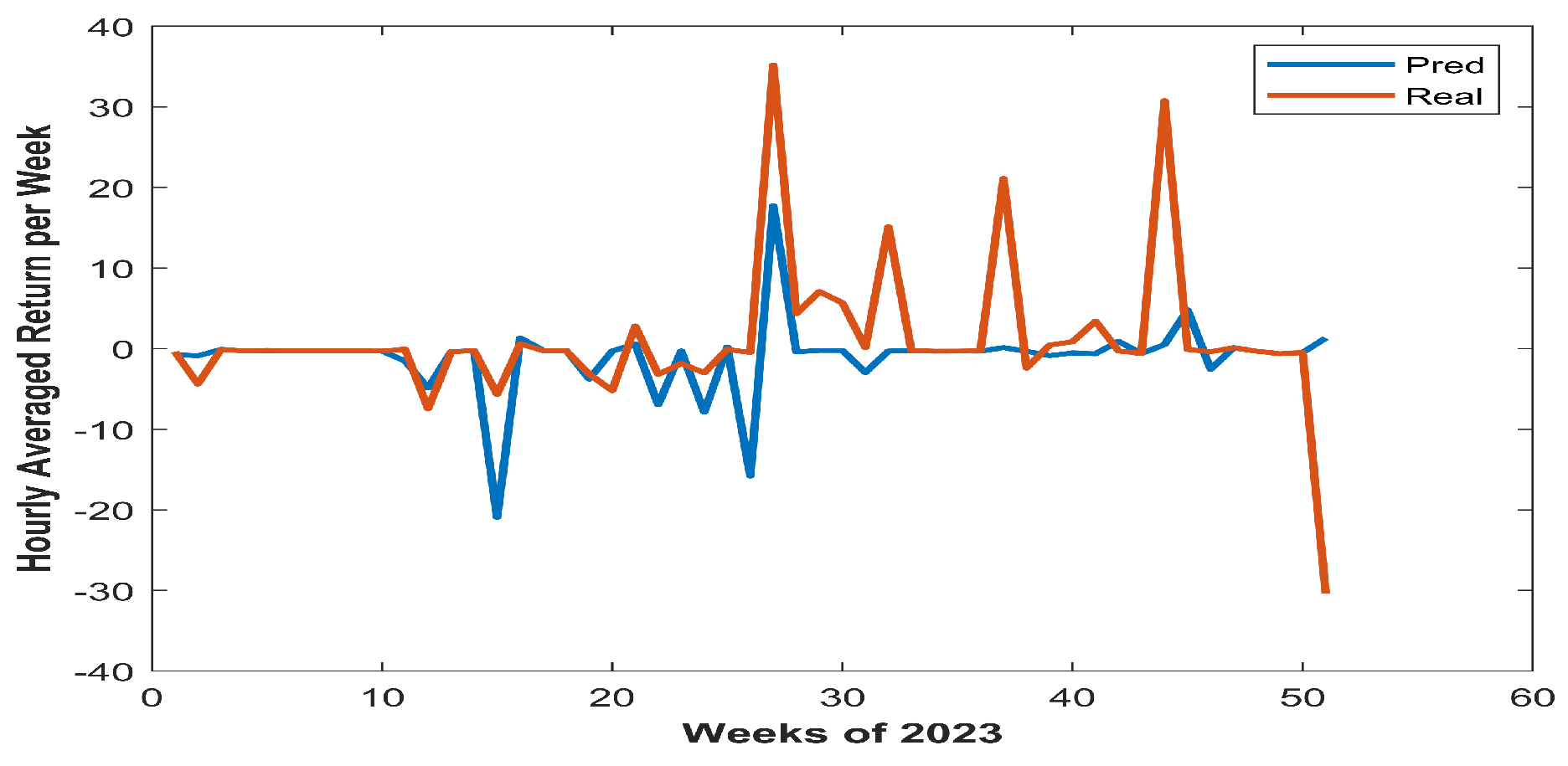
Figure 2.
Performance Evaluation
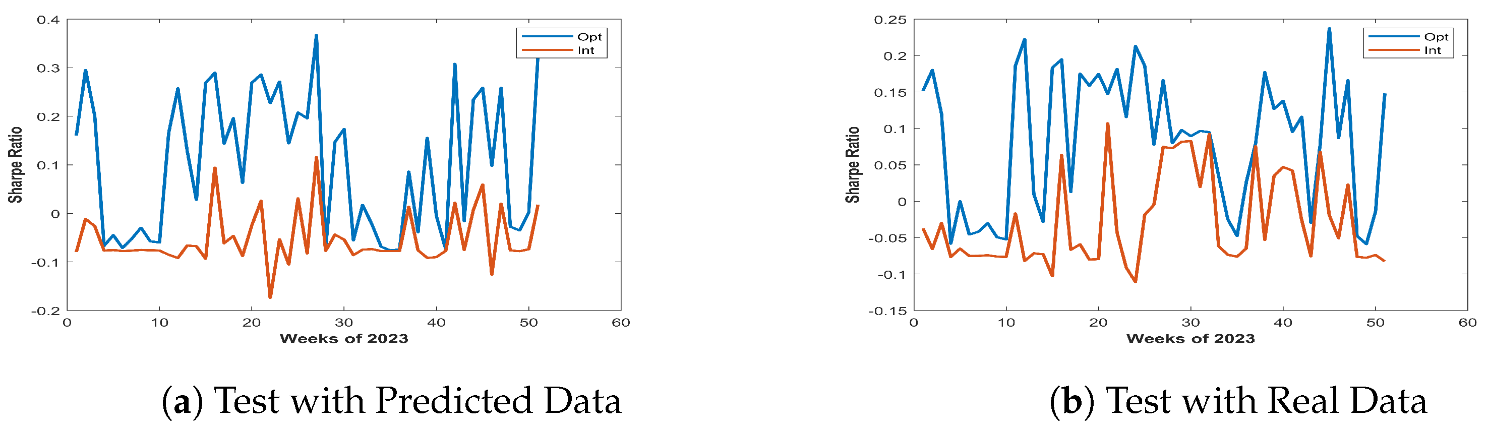
Figure 3.
VaR Evaluation
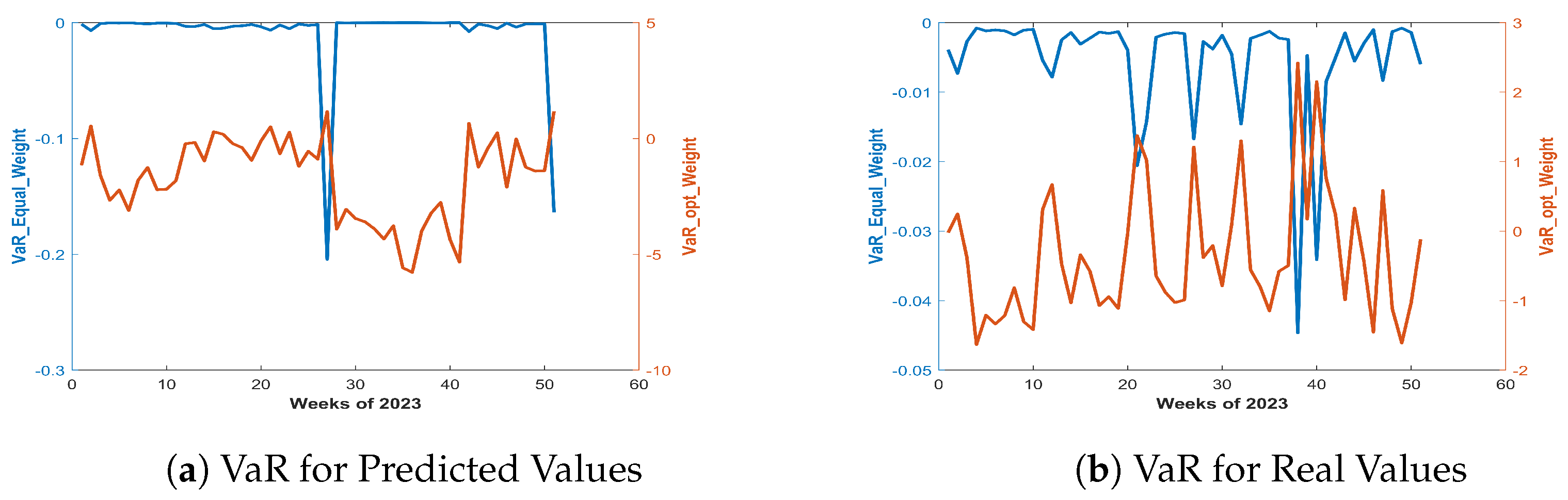
Figure 4.
CVaR Evaluation
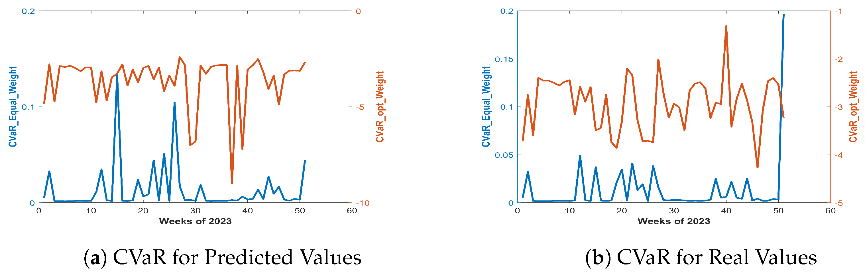
Figure 5.
Behaviour of CVaR with Different Values of and
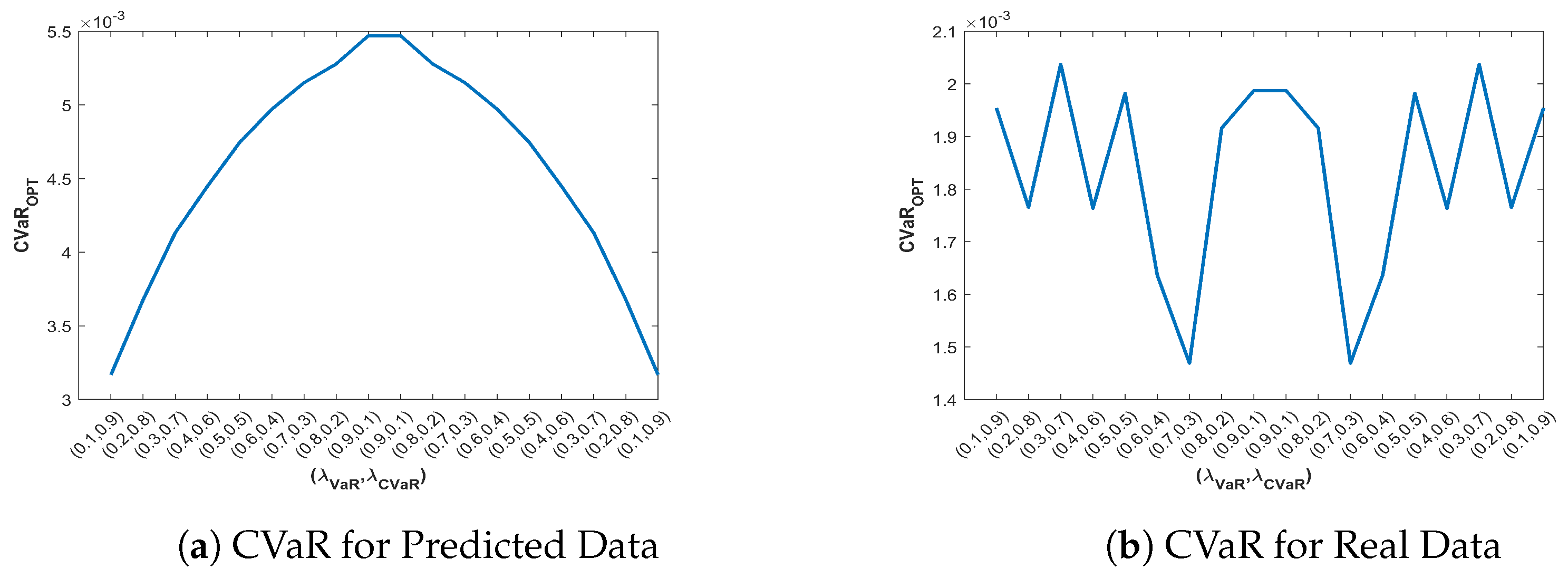
Figure 6.
Behaviour of VaR with Different Values of and

Figure 7.
Behaviour of Sharpe Ratio (SR) with Different Values of and
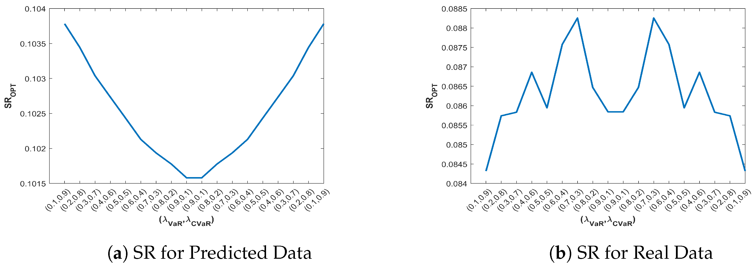

Table 1.
Combined Performance across different and settings
| Setting | ||||||
| Performance for & | ||||||
| Real Data | ||||||
| Predicted Data | ||||||
| Performance for & | ||||||
| Real Data | ||||||
| Predicted Data | ||||||
| Performance for & | ||||||
| Real Data | ||||||
| Predicted Data | ||||||
| Performance for & | ||||||
| Real Data | ||||||
| Predicted Data | ||||||
| Performance for & | ||||||
| Real Data | ||||||
| Predicted Data | ||||||
Table 2.
Comparison With Respect to Different Combination of and
| Real | -0.0054 | -1.2340 | 0.0131 | 0.0020 | -0.0289 | 0.0843 |
| Predicted | -0.0089 | -0.5427 | 0.0134 | 0.0055 | -0.0526 | 0.1016 |
Disclaimer/Publisher’s Note: The statements, opinions and data contained in all publications are solely those of the individual author(s) and contributor(s) and not of MDPI and/or the editor(s). MDPI and/or the editor(s) disclaim responsibility for any injury to people or property resulting from any ideas, methods, instructions or products referred to in the content. |
© 2024 by the authors. Licensee MDPI, Basel, Switzerland. This article is an open access article distributed under the terms and conditions of the Creative Commons Attribution (CC BY) license (http://creativecommons.org/licenses/by/4.0/).
Copyright: This open access article is published under a Creative Commons CC BY 4.0 license, which permit the free download, distribution, and reuse, provided that the author and preprint are cited in any reuse.


