Submitted:
28 November 2024
Posted:
28 November 2024
You are already at the latest version
Abstract
To explore the application of neural networks to estimate geomagnetic field disturbances, this study pays particular attention to K-index classification. The primary goal remains to provide a robust and efficient method for classifying the different levels of geomagnetic activity via neural networks. Data preprocessing, model architecture optimization, and classification performance evaluation are involved in this study at large. It proposes a new neural network method that attends to specific complexities of geomagnetic data and compares its merits against conventional methods. Neural networks, Long Short-Term Memory (LSTM) models in particular, revealed much better performance than traditional techniques with attained classification accuracy reaching 98%. The findings suggest that there is a promise for the applications of neural networks within geomagnetic studies and this will pave the way towards Artificial Intelligence models for forecasting or for the further inclusion of this approach to its articulation in discussions surrounding space weather research.
Keywords:
geomagnetic field
; geomagnetic disturbances
; neural networks
; k-index
1. Introduction
Geomagnetism [2,5], or Earth’s magnetism, is a specialized field within geophysics that explores the spatial distribution and temporal changes of the geomagnetic field, along with associated geophysical processes within the Earth and the upper atmosphere, as discussed in [1,3]. Studies like those by McCuen et al. [10] offer automated methods for detecting high-frequency geomagnetic disturbances, refining how we interpret field data and eliminating noise.
One of the fundamental aspects of the geomagnetic field involves its components and indices. Like any magnetic field, the geomagnetic field is defined by its strength F, which is quantified through its magnitude and direction. This is done by decomposing F into three orthogonal components—X, Y, and Z—within a rectangular coordinate system. According to Santos et al. [13], deep neural networks have proven effective in identifying flux rope signatures, enhancing space weather forecasting, which parallels studies on magnetic perturbations like those observed at Almaty Observatory [26].
As outlined in [7], the vector F (denoted as T in the source) is visually represented by a magnetic arrow suspended at the center of gravity (see Figure 1).
In this system, magnetic field consists of three components: X (northward, horizontal), Y (eastward, horizontal), and Z (vertical, downward). The total field strength, F, is the vector sum of these components, whilst H is the horizontal projection of F. Magnetic declination, D, is the angle between H and X, whereas magnetic inclination, J, is defined as the angle between H and F.
The components are important when studying the Earth’s magnetic field [4,6], as their changes influence geo-magnetic activity. Applications of the components involve navigation, geophysics, and space studies [27,28]. Changes in the magnetic field develop over time according to parameters such as latitude, season, and solar activity. This is differentiated into two types: slow or secular variations as influenced internal to the Earth, and fast variations that are in turn influenced by solar and magnetospheric effects [8].
There are several indices to quantify geomagnetic activity. The K-index, introduced in 1938, is a local measure quasi-logarithmic in character. It records magnetic activity over three-hour periods, from 0 (quiet) to 9 (severe storm). Each observatory has its charts for calculating K-indices, usually assigning a number greater than 4 to moderate or strong geomagnetic storms.
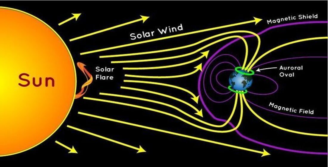
Geomagnetic disturbances are changes in the geomagnetic field that occur due to the influence of external factors on the Earth’s magnetic envelope. Such changes are caused by different factors such as solar wind [14] and geomagnetic storms[12,18]. This aligns with the present study’s focus on using neural networks to improve existing methodologies at Almaty Observatory, where Vega-Jorquera et al. [11] demonstrated how hybrid neural network models, enhanced with genetic algorithms, can forecast geomagnetic storms with high accuracy. Basically, the reason is that when the perturbed solar wind interacts with the magnetic field (Figure 2), it adds additional energy to the existing current system [20].
Due to advancements in science, modern society has become increasingly dependent upon power distribution networks and satellite systems that stand to lose connection due to geomagnetic disturbances-the disturbances that can interfere with GPS signals causing industries dealing with deep water drilling to suffer disruption[14,16]. Geomagnetically induced currents (GICs) are threats to power grids that can damage transformers resulting in prolonged outages. A notable example is the 1989 blackout that hit Quebec, when a magnetic storm caused power outages that lasted 9 hours. Knowing and predicting geomagnetic disturbances are vital for the security of critical infrastructure [30].
This study compares methodologies for predicting the extent of geomagnetic activity employing neural networks and tackles issues related to the not-so-resistant and inefficient method of work at the Almaty Geomagnetic Observatory. Neural networks are an area of great promise for enhancing the protection of technological infrastructures from geomagnetic disturbances. The research intends to construct an appropriate model for classifying disturbances by scrutinizing geomagnetic field data on an index called the K-index, a representative measure of geomagnetic activity.
This involves gaining insight into current disturbance estimation methods, acquiring relevant geomagnetic data, and developing a neural network model for the assessment of geomagnetic disturbances. Such a model will be trained with the input of real data to establish a high level of accuracy in predictions. The final stage of research entails testing the model and uncovering its merits and features of limitation.
Incorporating Kohonen’s neural networks into this context, as explored by Barkhatov et al. [17], highlights the potential to classify substorm activity based on interplanetary magnetic field changes, reinforcing the necessity of neural network applications in space weather. A neural network with an accuracy of about 95% is expected for geomagnetic disturbances. This work provides practical effects to improve protection systems and, theoretically, broadens knowledge of geomagnetic field dynamics and the use of neural networks in such applications to develop more reliable forecasting models for environments likely to face natural and technological disruptions [32,33].
2. Preparation for Building Neural Networks
2.1. Data Collection
The training data is a data set from the Almaty (Alma-Ata) geomagnetic Observatory, which is part of the Institute of Ionosphere of the National Research Center (Almaty, Republic of Kazakhstan). Observation data has been obtained from a LEMI-008 ferrosonde magnetometer, LEMI-203 portable single-component magnetometer, and a processor-based POS-1 Overhauser sensor.
This data set gives the results of the daily measurement of the geomagnetic field of the observatory from 2021 to 2023. Each file contains one block of 24 hours’ worth of data, which is parsed into a full 60 minutes of measurement. Included in the data set are: identifier of the observatory, date, ordinal day of the year, hour, components of the geomagnetic field, data type, code of the responsible organization, geographical coordinates, basic value of magnetic declination, and reserved fields[15]. The total amount of data is 1,576,800 records and 8 classes.
The magnetic data used to calculate geomagnetic activities were shown in Table 1:
The total amount of data is 1,576,800 records and 8 classes.
2.2. Data Preprocessing
In order to guarantee the correct use of data in their machine learning models and neural network setup, a numerically computed number of preliminary data processing works were performed [25].
First, the structural characteristics of data and the distribution of the K-index values were described, allowing for the identification of general levels of geomagnetic activity in the Almaty region [31]. The analysis suggested that K-index values did not exceed 7, while the most frequent values were 2, 3, and 1, showing in Table 2 a moderate level of environment disturbances in the region.
Data gaps have been addressed next. The distribution of variables was used as a factor in estimation of further gaps for the real analysis. For asymmetrically distributed data, the median value was selected for X, while for Z, the normal distribution was approached with the average being equal to all. For Y, F, and K-index, values with modal value extremes selected under the influence of the modal type of values inserted; this action seemed to preserve structural integrity and avoid distortions to the extent that this could influence analytical work or results. In Table 3 shown an example of a row in a dataset containing recorded magnetic parameters and K-index measurements:
To improve the stability and efficiency of the models, standardized data scaling was applied within the framework of the procedural plan, in which each variable is normalized by the average value and standard deviation. This approach also contributes to the accuracy of cross-validation in the following stages of modeling. Gaps were processed before using the data in machine learning tasks and neural networks.
In computing the number of missing values, analysis methods based on missing data were used. As a result of the studies, we obtained the following number of omissions for each variable: For variable X—15,802; for variable Y—15,802; for variable Z—15,802; for variable F—24,245; for variable K-index—20,703. Filling in the blanks was done considering the distribution of each variable. So, for a variable with a slightly asymmetric distribution, its median was used; for a variable with close to a normal distribution, the average value was used; for variables with pronounced modal values (modal values), the mode was used. Such filling allowed to preserve the structure and integrity of the data, as well as exclude distortions that can affect the analytical results.
Data standardization was performed by the StandardScaler method, which normalizes each feature by removing the mean and dividing by the standard deviation. This method standardizes a feature by subtracting the mean and dividing by the standard deviation. Thus, this method allows you to work with data in such a way that the mean is zero and the variance is one. This approach makes it possible to increase the stability and efficiency of the algorithms. Such a standardization method removes the mean and scales to the unit variance. These manipulations motivate a neural network to converge better during training and help to avoid overfitting.
2.3. Statistical Analysis
Administrative decisions to assess the parameters using Pearson’s correlation coefficient were based on the relationship between key parameters and the influence of seasonal variations on geomagnetic disturbances in 2022. The analysis enabled the quantification of the linear relationships between month, components X, Y, Z, and disturbance_estimation and it’s shown in the Figure 3.
In the month-’disturbance_estimation’ correlation, there is practically no connection at all. While the month received a correlation of 0.0338 again, the p-value is sufficiently greater than 0.05, highlighting the absence of the significant correlation. Thus, it can be concluded that the seasonal fluctuations by month hardly warrant any significant degree of influence on geomagnetic disturbances.
The relationship between X component and disturbance_estimation has been found to be negative moderately strong, for which the coefficient is -0.2935 and p-value of 0.0 suggest a significant feedback. This suggests that with the increase in value of component X, disturbance_estimation is decreased, which underlines the inverse relationship between these variables.
A weak positive correlation with disturbance_estimation was found for component Y, and though the correlation coefficient equaled 0.0082 and p-value was at a really low level of 3.19e-09, one could hardly say it would have had any meanings in the practical sense; so weak in connection is this. The Z component also yields a weak positive correlation with disturbance_estimation, with p-value at 0.0, which goes on to show at least a minimum but significant positive dependence.
In effect, the analysis revealed that different components of the magnetic field have ineradicable influence on the degrees of geomagnetic disturbances. Thereby, inversely, the X component has maximal impact, whereas both Y and Z components weakly correlate with disturbance_estimation.
Seasonal analysis is conducted to analyze the variation of K-index frequencies depending on the time of the year. Analysis of variance(ANOVA) was performed. ANOVA(2.5) a method aimed at finding dependencies in experimental data by examining the significance of differences in mean values:
where:
- is the standard deviation between groups(intergroup variance);
- SS within is the standard deviation within groups(within-group variance).
To ascertain the seasonal variation of K-index values, ANOVA with four seasons was carried, which helps to statistically infer the differences in the mean K-index values among the four seasons: Winter, Spring, Summer, and Fall.
The ANOVA was based on the following hypotheses:
- Null Hypothesis (H0): There would be no statistically significant differences in the K-index values across the seasons.
- Alternative Hypothesis (H1): Statistically significant differences exist in K-index values across at least two of the seasons.
The F-statistic calculated using ANOVA was 108.63, with a p-value of 2.61e-70. This gives a very small p-value. Hence, we reject the null hypothesis and conclude that significant differences exist among K-index values for the different seasons showmn in Figure 4.
This suggests that seasonal variation greatly influences geomagnetic disturbance. The visual representation supports the ANOVA results, indicating notable seasonal variations in geomagnetic activity.
2.4. Traditional Machine Learning Algorithm
The analysis of seasonal irregularities of geomagnetic disturbances was performed using two machine learning models: logistic regression and decision tree [22,24]. These serve as a starting point for learning about the plots and relations in the data [19,29].
Logistic regression encapsulated geomagnetic data within probabilistic model frameworks for seasonal variations [21]. Its simplicity and interpret ability made it suitable for exploratory analysis. For each season, a separate logistic regression model was constructed to capture the seasonal tendencies, where data subdivision was performed in the ratio of 70% for training and 30% for testing. Standard classification metrics evaluated model performance, thus giving indications as to how well the model could identify linear dependencies within the dataset.
Decision tree models were employed to capture more complicated forms of association between seasonal data and that from three years. The models were built with fixed hyperparameters including maximum depth of the tree, minimum samples per split, and minimum samples per leaf, which were specified for good accuracy optimization. Because of its hierarchical representation and simplicity of interpretation, the decision tree algorithm was well suited for exploration of the seasonal dependencies of geomagnetic activity.
These classical approaches thus laid down a very good base for the current understanding of the data and focused on the right predictors and relations that would form the base for analysis through advanced neural network models.
3. Building Neural Networks
The study used neural networks as a very powerful tool for analyzing and classifying geomagnetic disturbances [16,18]. Neural networks are uniquely capable of extricating complex patterns and interrelationships in larger volume datasets which aid in modeling and prediction work in geomagnetic studies [23]. The process of development mainly focused on creating a neural network architecturally suitable for the dataset and optimizing the performance with respect to various situations.
Thus, the first neural network built was intended for analyzing data for the year 2022. This model used a Multilayer Perceptron (MLP) architecture with three fully connected hidden layers. Each of these three hidden layers used the ReLU activation function to cure the vanishing gradient problem for more efficient training. Softmax was used in the output layer, which is very helpful for multiclass classification, stating probability estimates for the outputs. In this case, the model was trained using the Adam optimizer that can increase the learning rates dynamically to get faster convergence and more stable results. The categorical cross-entropy was selected as the loss function since it can fit multiclass classification problems very well. The combination of ReLU, Softmax, and Adam optimizer enriched the training process with robustness and interpretability.
To analyze seasonal variations in geomagnetic disturbances, separate neural networks were constructed for each season of 2022. These models featured dense architecture with less number of neurons in every layer, in addition to a dropout layer with a rate of 0.3 to prevent overfitting. The output layer consisted of eight neurons, one corresponding to each K-index class. It provided the networks an opportunity to learn field-specific seasonal patterns and dependence of the data[26]. The seasonal datasets themselves were of different sizes, varying from 84960 to 132480 rows, requiring ad-hoc training strategies for each one. The architectural design was aimed at computational efficiency and adaptiveness such that the network is able to process a variable volume of data effectively. Figure 5 shows the architecture of the seasonal neural network, while Table 5 describes the layer-wise construction.
To go beyond a one-year analysis, a meta-neural network has been formed, bringing into consideration everything-the data from 2021, 2022, and 2023. Designed to handle over 1,500,000 rows of data, this advanced architecture consists of six fully connected layers, a dropout layer, and one output layer. The architecture has 512 neurons in the first layer but reduces progressively in the other layers while ReLU activation was used to train the model more efficiently. So here, the dropout layer ensured that the network did not overfit so that the network could generalize well to the unseen data. The detail architecture of this network is shown in Table 6.
An 80–20 training-validation data split was applied throughout the training of all neural networks. The models did undergo training for a few epochs, and for each run, various batch sizes were used to improve efficiency and performance. The Adam optimizer helped by changing learning rates during training, thus boosting the speed and stability of convergence. The modeling architectures possessed dropout layers to address overfitting, thus adding to the robustness of the model. The ABM learners were able to adapt to working with ways of high dimensionality, seasonal changes, and varying nonlinear dependencies present in the geomagnetic data sets.
The introduction of temporal and seasonal information in the modeling neural networks facilitates modeling geomagnetic disturbances in a robust framework. Advanced architectures and robust learning techniques established in this study pave the way for useful enhancements in predictive applications of the future, such as showing the possibilities that future neural networks may introduce further into geomagnetic research.
Long Short-Term Memory (LSTM) for 2021–2023
The Long Short-Term Memory (LSTM) model has been developed for the analyzing and K-index forecasting through sequential and time-series data, especially benefitting from the advantages modeled by the sequential nature of the data [12,34]. Unlike standard machine learning algorithms, LSTM networks are specific in learning temporal dependencies, making them apt for capturing the subtle patterns endemic to geomagnetic activity over long periods of time.
The LSTM network consists of a series of connected gates: forget, input, update (cell state update), and output gates. These gates permit the network to choose, for every time step, what part of the information is retained and what is discarded, guaranteeing that information that is most pertinent courses its way through the network. By allowing selected information to be processed, LSTMs can deal with long-term dependencies, which is paramount for modeling time-series data such as the K-index.
The architecture of the LSTM model that was implemented comprised five stacked LSTM hidden layers with different numbers of neurons, with a fully connected dense layer normally after. This was supplemented by a dropout layer for regularization to tame overfitting. Eight neurons in the output layer decided the eight classifications of any level of geomagnetic disturbance intensities. Figure 6 illustrates the structural design of the LSTM model, while Table 7 summarizes the detailed architecture by layers.
Overrides for the hypermetrical parameters were properly setup for training the model. The epoch was limited to 50 and the batch size was set at 960 to ensure computational efficiency without adversely affecting the model’s learning capability. The total number of trainable parameters reached 565,300,856 and is indicative of the model’s high-dimensional construct from data.
The model was further improved with a dense layer following the LSTM layers, thus optimizing its usefulness in the extraction of non-linear patterns from data. The dropout layer enacted with a rate of 0.3 served as another regularization mechanism, working in a compelling manner to lower the probability of overfitting by switching off a small proportion of neurons in each forward pass of training.
Training was done using categorical cross-entropy loss function and the Adam optimizer, which worked in favor of categorical cross-entropy for effectively evaluating the model’s multi-class classification problem. The Adam optimizer dynamically adjusted learning rates proportional to the observed behaviors of gradients during optimization with an accelerated rate for convergence and stabilization of performances.
In a nutshell, the structure of the LSTM model was correctly designed to answer questions gleaned from sequential data analysis. Long-term retention of various dependencies with recurrent regularizations in training promoted U-turn suitability for complex time series predictions, exemplified by K-index forecasting.
The model was able to achieve unheard-of accuracy levels as evidenced by training and test data yielding a performance value as high as 98%. Moreover, this accuracy was complementary to the area under the ROC curve, demonstrating values close to one (i.e. 0.9992 for both training and test data), indicating a distinctly able classifier with little ability to misclassify between classes.
4. Results
To reach the aims and objectives of this study, various data analysis techniques were employed, including statistical analyses, traditional machine learning models, and advanced neural network modelling. This section presents the results of this analysis.
Composed solely of data for 2022, the initial dataset did not give satisfactory results through neural network analyses. The setup involved three hidden layers with fully connected neurons following ReLU activation functions and a Soft-max output layer: only 33% accuracy, with precision, recall, and F1 of 0% emphasized the ineptitude of the model for identifying the underlying data complexities. Thereafter, the proposal of building neural networks for each month was made so as to investigate if a more granular approach would achieve better results. Indeed, the strategy achieved outstanding improvements, with monthly models recording accuracy between 85% and 93%, pinpointing the fact that geomagnetic data patterns can vary significantly between months.
There was a suggestion that the traits of geomagnetic disturbances and variation in the seasons were interrelated. A correlation analysis showed that monthly variations showed little effect directly on the disturbance level, reinforcing the idea that the underlying components of the magnetic field could be more significant predictors. Seasonal analysis through ANOVA confirmed that cyclic patterns and trends were present in geomagnetic disturbances that correlated with seasonally empirically observed changes in natural processes. The results gave further reason for proceeding to the creation of specific models for each season.
Logistic regression and decision tree models were employed to further understand seasonal geomagnetic disturbances. Logistic regression, chosen for its simplicity and interpretability, demonstrated limited performance, with metrics ranging between 22% and 44%-indicating its inability to capture complex nonlinear dependencies in the data.
The other two decision trees required a minimum of data preprocessing and therefore performed significantly better, with average precision, recall, F1-scores, and accuracy exceeding 74%, peaking during autumn(Table 8). This showed that decision trees managed hyperparameter tuning well and adapted well to seasonal data. But ultimately, traditional methods were found insufficient to account for the more complicated temporal patterns of geomagnetic disturbances, thus motivating the study of neural networks.
Neural networks were developed in order to analyze geomagnetic disturbances at both seasonal and multi-year scales. Seasonal neural networks, trained on data from 2022, yielded desired results with an accuracy ranging between 96% and 99% for different seasons. Dense architectures with dropout layers were used in order to minimize overfitting while effectively capturing seasonal changes of geomagnetic activity(Table 9)
To enhance forecasting abilities, a neural network was employed on the multi-year data set, covering a period between 2021 and 2023. The architecture consisted of six fully connected layers, one dropout layer, and one output layer. The model delivered 97% accuracy with an F1 score between 90% and 91% and was highly robust, producing a ROC-AUC metric value of 0.997. This level of performance reflects the model’s vector path to the large datasets processed for geomagnetic disturbance forecasting.
After other models were evaluated, the LSTM model was applied to forecast the K-index for the second half of 2024. Thirty epochs were chosen to minimize computational demands. The model was training with a limited period, however still held high performance with precision, recall, F1 score, and accuracy being in the ranges of 92-94%, 92%, and 98%, respectively (Figure 7).
The prognosis showed little geomagnetic activity in the geomagnetic disturbance period. The vast majority of perturbations were of "Weak" and "Moderate" disturbance levels. The K-index reached a maximum of ”5" in July compared to 4 in August, with levels of 3 in June and October (Figure 8). Other months experienced conditions of stability reflected by a K-index of 2. These results highlight the expedience of developing geomagnetic disturbance models that recognize the temporal and seasonal nature of geomagnetic disturbances.
5. Discussion
This study reinforces the importance of seasonality and data granularity in predicting geomagnetic disturbances. The seasonal analysis produced salient cyclical trends and dependencies between the geomagnetic field and its external drivers. Classical machine learning models, such as logistic regression and decision trees, provided baseline insights but did not capture the highly complex nonlinear relationships existing in geomagnetic data.
Neural networks offered better performance than the traditional models, especially with respect to large-order temporal dependence. Seasonal neural network models performed consistently well for all seasons, establishing their ability to adapt to variations in geomagnetic activity. Extending the dataset over several years while introducing LSTM networks further improved model prediction results, highlighting the essence of analyzing long-term dependencies in time series data.
Expectations in predictive results for the second half of 2024 suggest that geomagnetic disturbances would stay less in this period between weak and moderate levels in any extremes. Yet the prediction bases itself on time and disturbance degree, thus the model lacks thoroughly considering exposition upsurges in disturbance models, e.g., solar flares and magnetospheric events.
Despite the compelling results, there are some limitations. First, the complexity of the computational design of an LSTM model can be substantially demanding hence not suitable for real-time application. Second, the models depend upon data in hand, with an often-lack of enough data for an idea of vital predictive features, such as solar activity measures. The future focus should incorporate larger datasets for increased accuracy and the comprehensiveness of future predictions.
The study thus underlines the great potential of machine learning in geomagnetic research and opens further applications, such as in space weather forecasting, earthquake prediction, and climate changes. The researchers can use neural networks to delve into insights from archived data sets, deriving insightful and actionable insights into the underlying dynamics of the Earth’s magnetic field.
6. Conclusions
Summarizing the research on the application of neural networks for the estimation of geomagnetic field disturbance, it is concluded that, despite existing methods for analyzing Earth’s magnetic disturbances, the use of neural networks is represented as a promising approach. At the beginning of the work, a thorough analysis of existing methods and approaches on this topic was carried out. This was necessary to identify possible limitations faced by current methods. This helped us to form a clear idea of which aspects require further improvement.
The models created have demonstrated high prediction accuracy, confirming their effectiveness in this context. Classical machine learning methods such as logistic regression and decision trees achieved good results, but neural networks, especially Long short-term memory, proved to be the most precise and adaptive in predicting geomagnetic anomalies, with an accuracy of 98%.
At the end of this study, it can be said that all the aims and objectives have been achieved. This work confirmed the potential of neural networks in the field of forecasting geomagnetic disturbances, but requires further research and improvement. For example, by supplementing the data with such important factors as solar flares, coronal mass ejections, etc., and using more powerful hardware, more accurate and reliable results can be achieved.
Author Contributions
For research articles with several authors, a short paragraph specifying their individual contributions must be provided. The following statements should be used “Conceptualization, M.N. and B.Z.; methodology, M.N.; software, A.A and D.Z.; validation, A.A. and M.N.; formal analysis, A.A.; investigation, M.N.; resources, B.Z. and V.K; data curation, B.Z. and V.K; writing—original draft preparation, M.N.; writing—review and editing, A.A. and D.Z; visualization, D.Z.and V.K; supervision, M.N.; project administration, B.Z. Authors have read and agreed to the published version of the manuscript.
Funding
Funding was supported by grant funding from the Science Committee of the Ministry of Science and Higher Education of the Republic of Kazakhstan (AP19679336).
Data Availability Statement
The training data for this study were obtained from the Almaty Geomagnetic Observatory, which is a part of the Institute of Ionosphere of the National Research Center (Almaty, Republic of Kazakhstan). The dataset contained daily measurements of geomagnetic field components from 2021 to 2023 using LEMI-008 ferrosonde magnetometer, LEMI-203 portable single-component magnetometer, and a processor-based POS-1 Overhauser sensor. These data are not publicly available but will be provided upon reasonable request, at the discretion of the responsible organization.
Conflicts of Interest
The authors declare no conflicts of interest.
References
- Vologda Regional Universal Scientific Library - VOUNB. Available online: https://www.booksite.ru/fulltext/1/001/008/046/103.htm.
- “Magnetic field,” Atomic Energy. Available online: https://atombit.org/magnitnoe-pole/.
- Tiwari, P. Geomagnetism: Discoveries and developments in the past. Geography Notes 2024. [Google Scholar]
- Dr. David P. Stern Early history of electricity and magnetism. http://www.phy6.org/Electric/-E14-history.htm.
- Parkinson, W.D. Introduction to Geomagnetism. Edinburgh: Scottish Academic Press, 1983.
- Geomagnetic Field and the Evolution of the Earth. Available online: https://www.phys.msu.ru/rus/about/sovphys/ISSUES-2006/6(53)-2006/53-4/.
- The Sun, Magnetic Storms, the Biosphere and Man. Available online: https://ukhtoma.ru/dinamic7.htm.
- The Editors of Encyclopædia Britannica, “Geomagnetic storm,” Encyclopædia Britannica. Available online: https://www.britannica.com/science/geomagnetic-storm.
- NASA. Solar wind magnetic field interaction with the Earth’s magnetic field. Image from: Ningchao Wang, "Lagrangian Coherent Structures in Ionospheric-Thermospheric Flows," Doctoral Dissertation, Illinois Institute of Technology, Chicago, Illinois, July 2018.
- McCuen, B.A.; Moldwin, M.B.; Steinmetz, E.S.; Engebretson, M.J. Automated high-frequency geomagnetic disturbance classifier: A machine learning approach to identifying noise while retaining high-frequency components of the geomagnetic field. Journal of Geophysical Research: Space Physics 2023, 10, 128. [Google Scholar] [CrossRef]
- Vega-Jorquera, P.; Lazzús, J.A.; Rojas, P. GA-optimized neural network for forecasting the geomagnetic storm index. Geofísica Internacional 2018, 10, 239–251. [Google Scholar] [CrossRef]
- Wihayati, W.; Purnomo, H.D.; Trihandaru, S. Disturbance Storm Time Index Prediction using Long Short-Term Memory Machine Learning. Proceedings - 2021 4th International Conference on Computer and Informatics Engineering: IT-Based Digital Industrial Innovation for the Welfare of Society (IC2IE 2021); IEEE, Virtual, Depok, 14 September 2021; pp. 311–316. [CrossRef]
- dos Santos, L.F.G.; Narock, A.; Nieves-Chinchilla, T.; Nuñez, M.; Kirk, M. Identifying Flux Rope Signatures Using a Deep Neural Network. Solar Physics 2020, 295, 131. [Google Scholar] [CrossRef]
- Pick, L.; Effenberger, F.; Zhelavskaya, I.; Korte, M. A Statistical Classifier for Historical Geomagnetic Storm Drivers Derived Solely From Ground-Based Magnetic Field Measurements. Earth and Space Science 2019, 6, 2000–2015. [Google Scholar] [CrossRef]
- Geppener, V.V.; Mandrikova, O.V.; Zhizhikina, E.A. Automatic method for estimation of the earth’s Magnetic Field State. In 2015 XVIII International Conference on Soft Computing and Measurements (SCM), 2015, 10, 2000–2015. [Google Scholar]
- Siddique, T.; Mahmud, M.S. Ensemble deep learning models for prediction and uncertainty quantification of ground magnetic perturbation. Frontiers in Astronomy and Space Sciences 2022, 10, 2000–2015. [Google Scholar] [CrossRef]
- Barkhatov, N.A.; Revunov, S.E.; Cherney, O.T.; Mukhina, M.V.; Smirnova, Z.V. Neural networks technique for detecting current systems while main phase of geomagnetic storm. E3S Web of Conferences 2020, 10, 2000–2015. [Google Scholar] [CrossRef]
- Tasistro-Hart, A.; Grayver, A.; Kuvshinov, A. Probabilistic geomagnetic storm forecasting via Deep Learning. Journal of Geophysical Research: Space Physics 2021, 10, 2000–2015. [Google Scholar] [CrossRef]
- Liu, G.; et al. Automatic classification and recognition of geomagnetic interference events based on machine learning. Journal of Computational Methods in Sciences and Engineering 2022, 10, 1157–1170. [Google Scholar] [CrossRef]
- Zerbo, J.L.; Amory Mazaudier, C.; Ouattara, F.; Richardson, J.D. Solar wind and geomagnetism: Toward a standard classification of geomagnetic activity from 1868 to 2009. Annales Geophysicae 2012, 10, 421–426. [Google Scholar] [CrossRef]
- Pinto, V.A.; et al. Revisiting the ground magnetic field perturbations challenge: A machine learning perspective. Frontiers in Astronomy and Space Sciences 2022, 10, 421–426. [Google Scholar] [CrossRef]
- Géron, A. Hands-On Machine Learning with Scikit-Learn, Keras, and TensorFlow, 2nd Edition; O’Reilly Media: Sebastopol, 2019.
- Chollet, F. Deep Learning with Python; Manning Publications: Sebastopol, 2021. [Google Scholar]
- Müller, A.C.; Guido, S. Introduction to Machine Learning with Python: A Guide for Data Scientists; O’Reilly Media: Sebastopol, 2018. [Google Scholar]
- Altaibek, A.; Tokhtakhunov, I.; Nurtas, M.; Kozhamzharova, D.; Aitimov, M. The Efficacy of Autoencoders in the Utilization of Tabular Data for Classification Tasks. Proc. Comput. Sci. 2024, 238, 492–502. [Google Scholar] [CrossRef]
- Mashakova, D.; Nurtas, M.; Ydyrys, A.; Ipalakova, M. Improving Weather-Sensing Uncrewed Aerial Vehicles with Machine Learning Prediction Models. CEUR Workshop Proceedings, 2023, 3680, Almaty. [Google Scholar]
- Nurtas, M.; Zhantaev, Z.; Altaibek, A. Earthquake Time-Series Forecast in Kazakhstan Territory: Forecasting Accuracy with SARIMAX. Procedia Computer Science, 2023, 231, 353–358. [Google Scholar] [CrossRef]
- Nurtas, M.; Zhantaev, Z.; Altaibek, A.; Nurakynov, S.; Mekebayev, N.; Shiyapov, K.; Iskakov, B.; Ydyrys, A. Predicting the Likelihood of an Earthquake by Leveraging Volumetric Statistical Data Through Machine Learning Techniques. Engineered Science, 2023, 26. [Google Scholar] [CrossRef]
- Nurtas, M.; Ydyrys, A.; Altaibek, A. Using of Machine Learning Algorithm and Spectral Method for Simulation of Nonlinear Wave Equation. ACM International Conference Proceeding Series, 2020, 6th International Conference on Engineering and MIS (ICEMIS 2020), Almaty, Kazakhstan, 14–16 September 2020. [CrossRef]
- Meirmanov, A.; Nurtas, M. Mathematical Models of Seismics in Composite Media: Elastic and Poro-Elastic Components. Electronic Journal of Differential Equations, 2016, 12 July 2016. Available online: https://ejde.math.txstate.edu/Volumes/2016/116/.
- Salikhov, N.; Shepetov, A.; Pak, G.; Nurakynov, S.; Ryabov, V.; Sadyuev, N.; Sadkov, T.; Zhantaev, Z.; Zhukov, V. Monitoring of Gamma Radiation Prior to Earthquakes in a Study of Lithosphere-Atmosphere-Ionosphere Coupling in Northern Tien Shan. Atmosphere 2022, 13, 1667. Available online: https://www.mdpi.com/20734433/13/10/1667. [CrossRef]
- Issakhov, A.; Abylkassymova, A.; Issakhov, A. Simulation of conjugate convective heat transfer in a vertical channel with thermal conductivity property of the solid blocks under the effect of buoyancy force. Numerical Heat Transfer, Part A: Applications 2024. [Google Scholar] [CrossRef]
- Issakhov, A.; Zhandaulet, Y.; Abylkassymova, A.; Issakhov, A. A numerical simulation of air flow in the human respiratory system for various environmental conditions. Theoretical Biology and Medical Modelling 2021, 18. [Google Scholar] [CrossRef] [PubMed]
- Altaibek, A.; Nurtas, M.; Zhantayev, Z.; Zhumabayev, B.; Kumarkhanova, A. Classifying Seismic Events Linked to Solar Activity: A Retrospective LSTM Approach Using Proton Density. Atmosphere 2024, 15. [Google Scholar] [CrossRef]
Figure 1.
Geomagnetic field components.
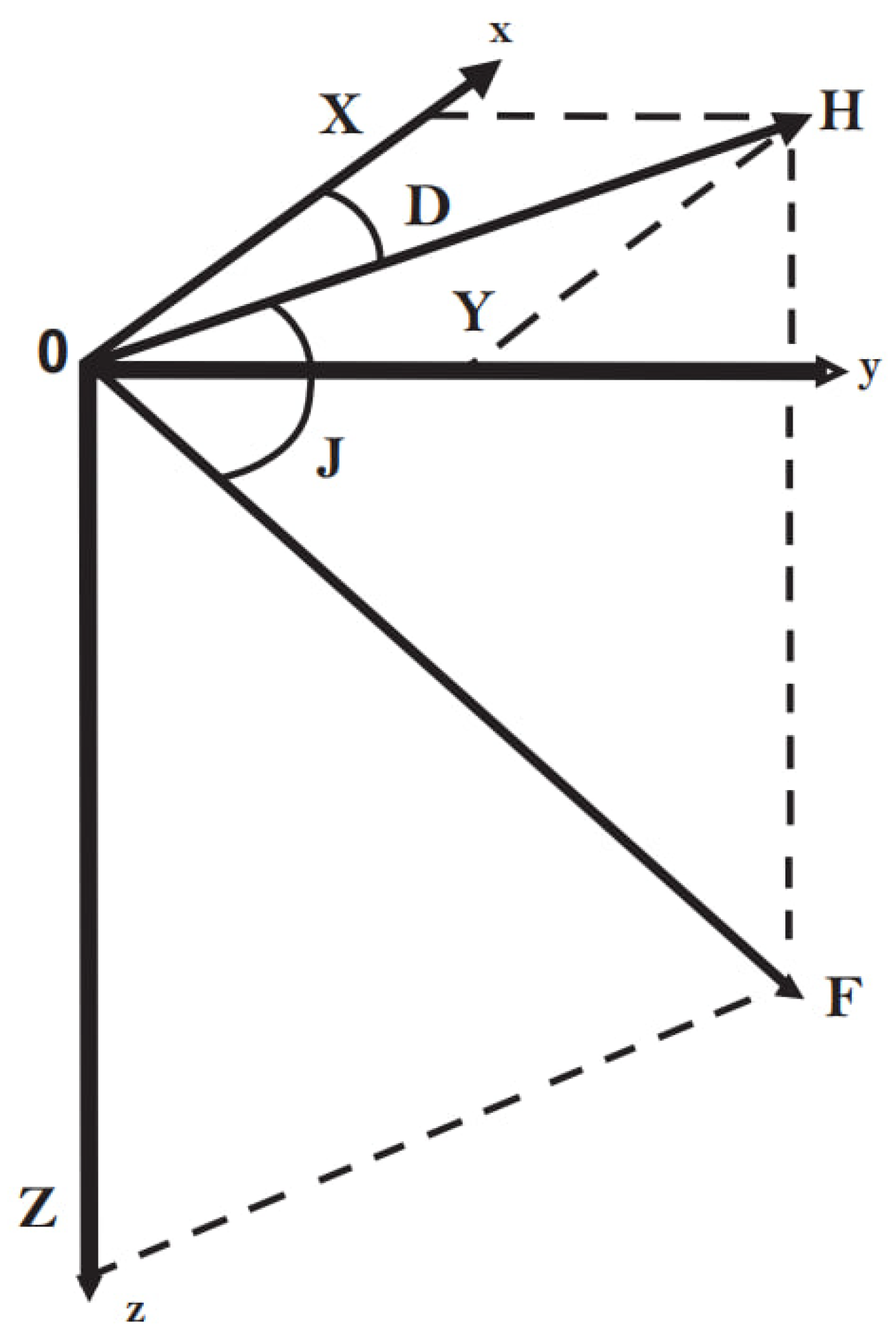
Figure 2.
Interaction of Earth’s magnetic field with solar wind [9].
Figure 2.
Interaction of Earth’s magnetic field with solar wind [9].

Figure 3.
Correlation Heatmap of Geomagnetic Field Components and K-index.
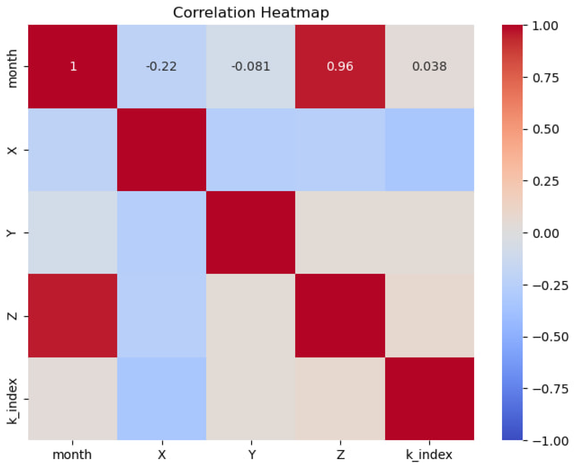
Figure 4.
Seasonal Variation in K-index Values.
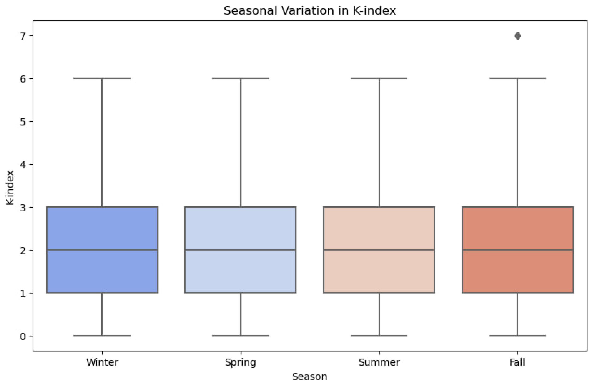
Figure 5.
Architecture of Neural Network model for 4 seasons of 2022.
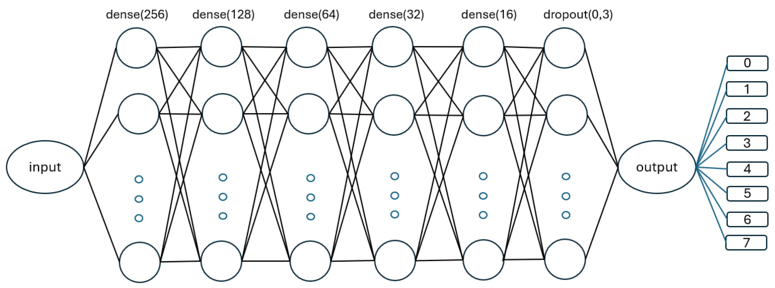
Figure 6.
Architecture of LSTM for 2021–2023.
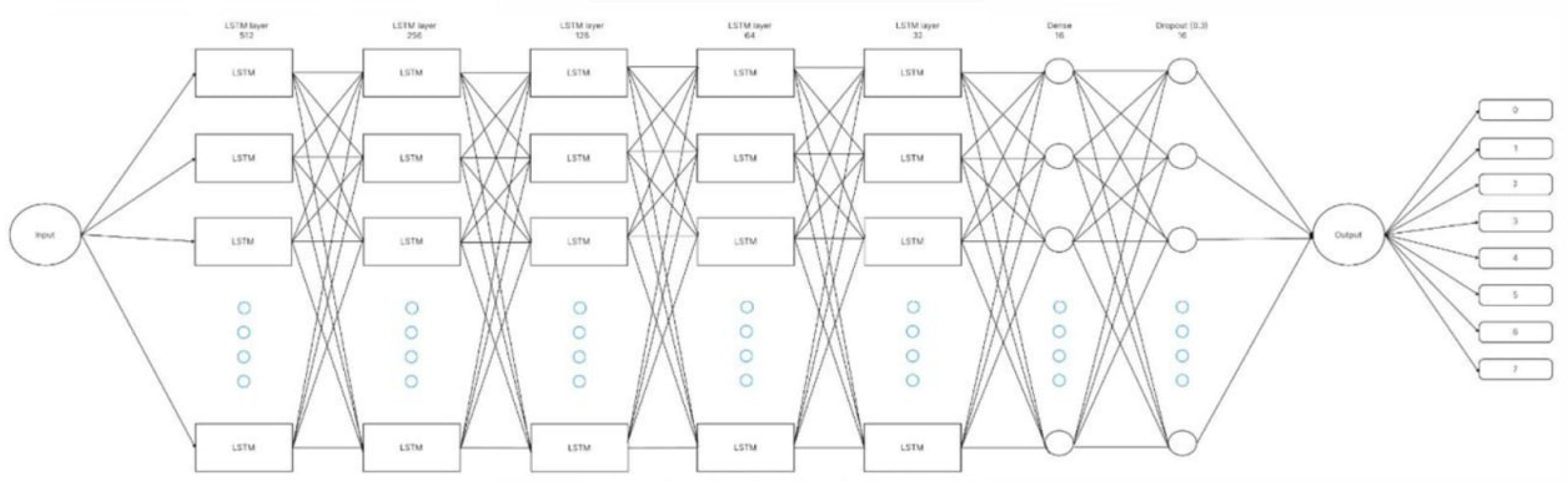
Figure 7.
Max K-index for each month of 2024.
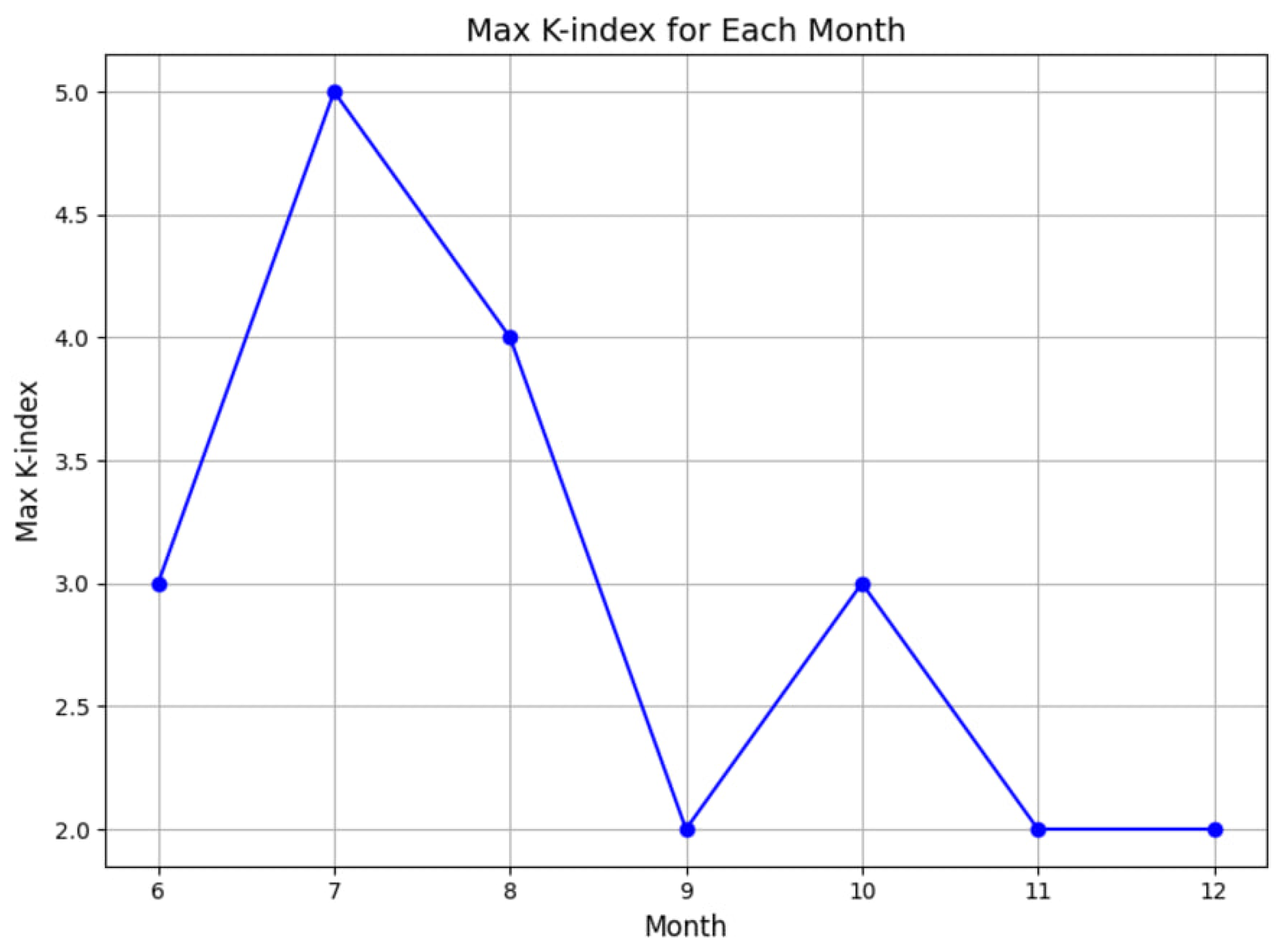
Figure 8.
Max K-index for each month of 2024.
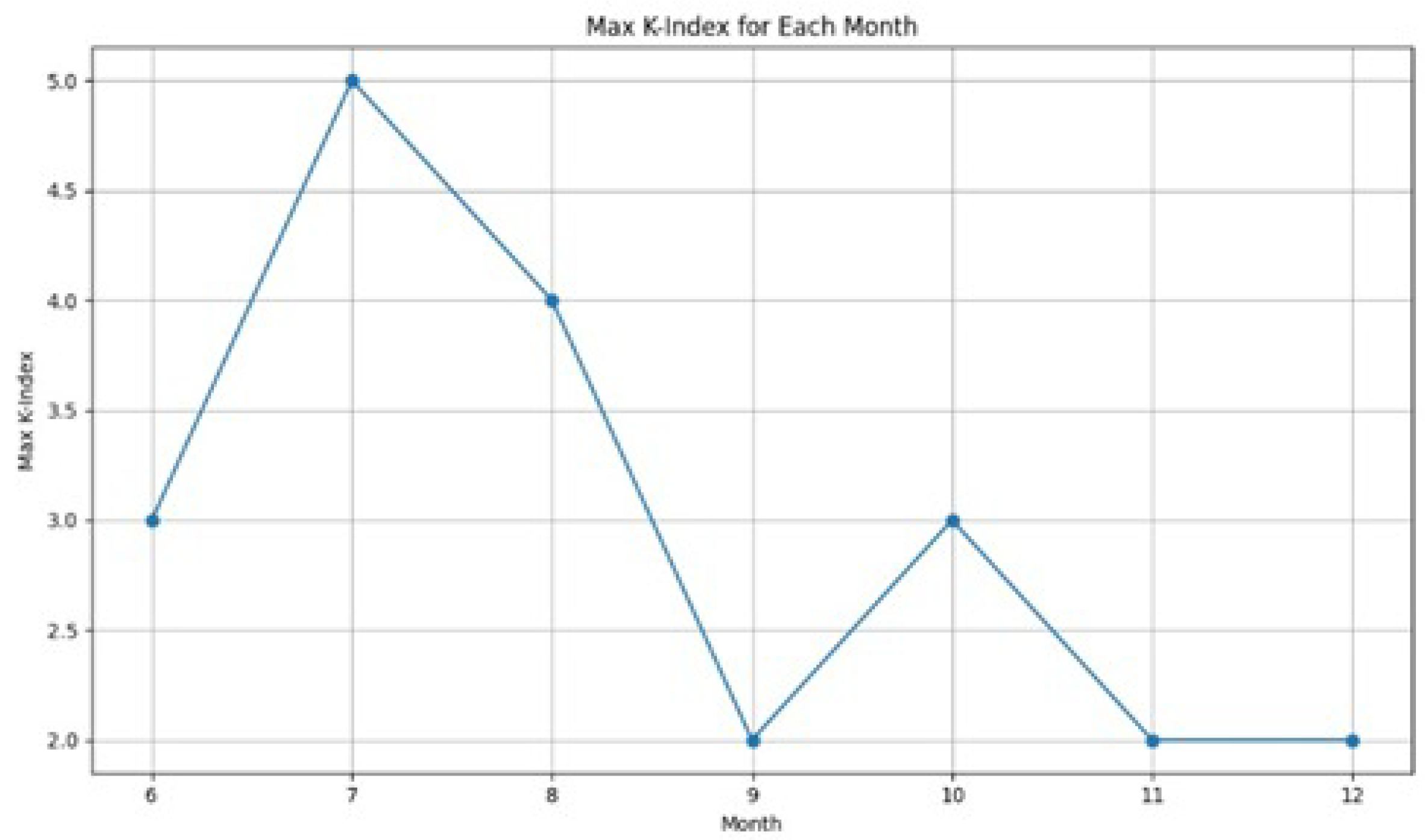

Table 1.
The magnetic data for calculation geomagnetic activities.
| Parameters | Description | Range of Value |
|---|---|---|
| Year | Year | 2021–2023 |
| Month | Month of measurements | 1–12 |
| Day | Measurement day | 1–31 |
| Hour | Measurement hour | 0–23 |
| Minute | Minute of measurements | 1–60 |
| X | Direction of the north-south magnetic field, measured in tenths of a nanotesla | - |
| Y | Direction of the magnetic field east-west, measured in tenths of a nanotesla | - |
| F | The total intensity of the magnetic field, measured in nanotesla | - |
| K-index | An indicator for assessing geomagnetic activity | 0–7 |
Table 2.
Frequency of the K-index values.
| K-Index | Frequency |
|---|---|
| 2.0 | 505197 |
| 1.0 | 417600 |
| 3.0 | 343500 |
| 4.0 | 127500 |
| 0.0 | 109800 |
| 5.0 | 43500 |
| 6.0 | 7020 |
| 7.0 | 1980 |
Table 3.
Example of a row in a dataset containing recorded magnetic parameters and K-index measurements.
Table 3.
Example of a row in a dataset containing recorded magnetic parameters and K-index measurements.
| Year | Month | Day | Hour | Minute | X | Y | Z | F | K-index | |
|---|---|---|---|---|---|---|---|---|---|---|
| 0 | 2021 | 1 | 1 | 0 | 1 | −370.0 | 419.0 | 3606.0 | 554599.0 | 0.0 |
| 1 | 2021 | 1 | 1 | 0 | 2 | −370.0 | 420.0 | 3606.0 | 554599.0 | 0.0 |
| 2 | 2021 | 1 | 1 | 0 | 3 | −369.0 | 422.0 | 3606.0 | 554600.0 | 0.0 |
| 3 | 2021 | 1 | 1 | 0 | 4 | −368.0 | 425.0 | 3607.0 | 554601.0 | 0.0 |
| 4 | 2021 | 1 | 1 | 0 | 5 | −369.0 | 427.0 | 3607.0 | 554600.0 | 0.0 |
Table 4.
Classification of geomagnetic activity based on K-index.
| The Level of Disturbance | The Value of the K-Index |
|---|---|
| Very weak | 0 |
| Weak | 1–2 |
| Moderate | 3–4 |
| Significant | 5 |
| Strong | 6–7 |
Table 5.
Layer-wise model structure for K-index classification for 4 seasons of 2022.
| Layer | Input Values | Output Values | Number of Weights | Number of Biases |
|---|---|---|---|---|
| Dense(256) | 59,472-92,736 | 256 | 15,224,832-23,740,416 | 256 |
| Dense(128) | 256 | 128 | 32,768 | 128 |
| Dense(64) | 128 | 64 | 8,192 | 64 |
| Dense(32) | 64 | 32 | 2,048 | 32 |
| Dense(16) | 32 | 16 | 512 | 1 6 |
| Dropout(0.3) | 16 | 16 | 0 | 0 |
| Output(7-8) | 16 | 7-8 | 112-128 | 7-8 |
Table 6.
Architecture of Neural Network.
| Layer | Input Values | Output Values | Number of Weights | Number of Biases |
|---|---|---|---|---|
| Dense(512) | 1,103,760 | 512 | 565,125,120 | 512 |
| Dense(256) | 512 | 256 | 131,072 | 256 |
| Dense(128) | 256 | 128 | 32,768 | 128 |
| Dense(64) | 128 | 64 | 8,192 | 64 |
| Dense(32) | 64 | 32 | 2,048 | 32 |
| Dense(16) | 32 | 16 | 512 | 1 6 |
| Dropout(0.3) | 16 | 16 | 0 | 0 |
| Output(8) | 16 | 8 | 128 | 8 |
Table 7.
Table based architecture of LSTM for 2021–2023.
| Layer | Input Values | Output Values | Number of Weights | Number of Biases |
|---|---|---|---|---|
| LSTM(512) | 1,103,760 | 512 | 565,125,120 | 512 |
| LSTM(256) | 512 | 256 | 131,072 | 256 |
| LSTM(128) | 256 | 128 | 32,768 | 128 |
| LSTM(64) | 128 | 64 | 8,192 | 64 |
| LSTM(32) | 64 | 32 | 2,048 | 32 |
| Dense(16) | 32 | 16 | 512 | 1 6 |
| Dropout(0.3) | 16 | 16 | 0 | 0 |
| Output(8) | 16 | 8 | 128 | 8 |
Table 8.
Performance of Decision tree model of all seasons and three-year period
| Season/Period | Max Depth | Min Samples Split | Min Samples Leaf | Precision (%) | Recall (%) | F1-score (%) | Accuracy (%) |
|---|---|---|---|---|---|---|---|
| Winter | 10 | 5 | 10 | 77–78 | 73–74 | 74–75 | 74 |
| Spring | 12 | 5 | 10 | 80 | 74 | 79–80 | 79–80 |
| Summer | 12 | - | - | 82–83 | 77–78 | 81–83 | 82–83 |
| Autumn | 13 | - | - | 86–87 | 88 | 86–87 | 86–87 |
| Three-year period | 20 | 10 | 20 | 83–84 | 79–80 | 82–83 | 83–84 |
Table 9.
Results of NN for seasons.
| Season | Precision | Recall | PF1-score | Accuracy |
|---|---|---|---|---|
| Winter | 96–100% | 90–100% | 95–100% | 99% |
| Spring | 86–100% | 91–100% | 93–99% | 98–99% |
| Summer | 96% | 96% | 96% | 96% |
| Autumn | 97% | 97% | 97% | 99% |
Disclaimer/Publisher’s Note: The statements, opinions and data contained in all publications are solely those of the individual author(s) and contributor(s) and not of MDPI and/or the editor(s). MDPI and/or the editor(s) disclaim responsibility for any injury to people or property resulting from any ideas, methods, instructions or products referred to in the content. |
© 2024 by the authors. Licensee MDPI, Basel, Switzerland. This article is an open access article distributed under the terms and conditions of the Creative Commons Attribution (CC BY) license (http://creativecommons.org/licenses/by/4.0/).
Copyright: This open access article is published under a Creative Commons CC BY 4.0 license, which permit the free download, distribution, and reuse, provided that the author and preprint are cited in any reuse.


