Submitted:
27 November 2024
Posted:
28 November 2024
You are already at the latest version
Abstract
The grain yield in China’s Northeast black soil region represents 1/4 of the national total, resulting in an annual pesticide usage of about 190,000 tons. Pesticide identification is crucial for maintaining the health of black soil. Due to low gas volume and low concentration of pesticide volatile gas in black soil, the traditional vertical electronic noses (E-nose) cannot effectively capture them. To address this issue, we proposed an externally driven vortex E-nose that achieves improved performance. Through multi-objective optimization strategy using computational fluid dynamics (CFD), response surface methodology (RSM), and non-dominated sorting genetic algorithm II (NSGA-II), vortex E-nose was obtained, with an average velocity of 0.117 m/s and an average vorticity of 133.175 s-1 around sensors. The 3D-printed sampling chamber, with a volume of only 81.447 cm³, supports portable applications. Furthermore, pesticide odor information captured by vortex E-nose is analyzed using a convolutional neural network (CNN) algorithm. Experimental results show that vortex E-nose achieves 100% accuracy in identifying pesticide types and 97.62% in detecting pesticide components in black soil. The vortex E-nose we designed has potential advantages in trace gas detection environments.
Keywords:
vortex
; electronic nose
; gas detection
; pesticides identification
; soil pollution
1. Introduction
As China’s largest commodity grain production base, the Northeast Black Soil Region accounts for one-fourth of the country’s total grain output. However, the increase in crop yields in this region is inseparable from the extensive use of pesticides. According to statistics, the annual usage of pesticides in the Northeast Black Soil Region has reached up to 190,000 tons in recent years [1]. Due to the influence of latitude and temperature, pesticides in black soil are difficult to degrade and volatilize. Years of accumulated pesticides have seriously polluted soil and affected human health throughout the food chain [2,3,4]. Accurately identifying pesticide pollution in black soil is a prerequisite for properly managing and restoring soil in the Northeast Black Soil Region.
Currently, advanced sensing technologies used for soil pesticide pollution detection mainly focus on detecting volatile gas in pesticides, including electrochemical, optical, and enzyme-based biosensors [5,6]. However, these sensing technologies face challenges such as high costs, large sizes, poor real-time capabilities, and complicated pretreatment processes, preventing the realization of in-situ, real-time, and accurate identification of pesticide contamination in soil. In recent years, electronic nose (E-nose) technology has integrated sensors with nanoscale gas-sensitive materials, enabling in situ, real-time detection of complex gases. This technology offers significant advantages, such as small size, low cost, and simple operation [7,8,9].
Unfortunately, the amount of gas volatilized from pesticide residues in black soil is minimal, and its concentration is low, making it difficult for E-nose to effectively capture gas molecules. The conventional approach to address this issue is to enhance the concentration of volatile gases through enrichment, thereby improving the identification performance of e-nose. However, the adsorption materials used in enrichment have a short lifespan, and the desorption process consumes a lot of power, significantly increasing both costs and time [10]. A sampling chamber equipped with a sensor array can concentrate gas in a fixed area, allowing for rapid and continuous identification without enrichment, thus greatly improving effectiveness.
To ensure full contact between E-nose and gas molecules, the design of the sampling chamber must ensure a low-velocity, high-vortex airflow around sensors. Most research focuses on the design of the internal flow-guiding structure of the chamber. For example, Cheng, Dohare, et al. [11,12] use internal baffles to redistribute the airflow; Viccione et al. [13] incorporate diffusion structures at inlet and outlet to reduce dead zones where airflow stagnates; Wang et al. [14] use biomimetic concepts to design internal flow paths based on biological structures. However, improving the internal structure of the sampling chamber is costly and difficult to process and maintain. A simple external design can achieve the same sampling effect. Chang et al. [15] introduced a vertical jet flow into the sampling chamber, allowing airflow to interact with the surrounding sensors, achieving good results. However, this design leads to excessively fast airflow around the sensors, with low vortex intensity, while the chamber’s strong diffusion effect hinders the sensor array’s ability to capture airflow. The sampling chamber with a tangential inlet avoids these issues above by generating vortex jet flow. It generates a hollow structure with tangential vortex flow inside the chamber, creating low-velocity, high-vortex regions near the inner walls [16,17]. We apply this characteristic to the design of E-nose. On the one hand, it is important to consider the impact of the chamber inlet structure and flow rate on shape of vortex flow. On the other hand, the airflow conditions at the sensor installation location must also be considered.
Thus, the key to the design of the E-nose is to cleverly use the tangential inlet of the sampling chamber to generate vortices, allowing sensors to effectively capture gas molecules. Compared to our previous report, this paper presents a vortex E-nose that improves the accurate identification of pesticides in black soil, as described below. The structure of this paper is as follows.
- Structural Design: Based on gas jet theory, a vortex E-nose with an externally driven chamber structure was designed to achieve vortex flow within the sampling chamber.
- Optimization Method: Response surface methodology (RSM) and non-dominated sorting genetic algorithm II (NSGA-II) are combined for multi-objective optimization. The results of optimization and simulation of the portable E-nose show a small error.
- Performance Evaluation: The vortex E-nose, using the convolutional neural network (CNN) algorithm, accurately identified pesticide types and components in black soil.
Section 2 details experimental sample preparation, vortex E-nose Design, multi-objective optimization strategy, and pesticide identification and evaluation methods. Section 3 assesses the vortex E-nose’s optimization design process and experimental performance. Section 4 concludes the paper, highlighting the potential of vortex E-nose in practical applications.
2. Materials and Methods
2.1. Soil Samples Preparation
Pesticides such as organophosphates, organosulfurs, and pyrethroids are widely used in black soil. Two representative pesticide components from these three types were chosen as research subjects for this study. As shown in Figure 1, these pesticides were purchased from the pesticide market in Changchun City, Jilin Province, China. Black soil used for pollution identification tests was collected from the experimental farmland of Jilin University (43°N, 125°E). The selected black soil was dried and sieved, with an organic matter content of 47.4 g/kg and a pH value of 7.15, and was confirmed to be healthy soil free of any pesticides. Next, an artificial leaching experiment was conducted to simulate the working conditions of E-nose in pesticide detection in black soil [18]. Six black soil samples contaminated with pesticides and one control group using distilled water instead of pesticides were obtained.
The experimental procedure was as follows: first, a leaching column was filled with 10 cm of soil, then compacted and moistened. Next, 2 mL of pesticide dilution, prepared according to the recommended usage dosage and dilution ratio, was evenly dripped onto the soil surface. Subsequently, 800 mL of 0.01 mol/L CaCl2 solution was used to simulate rainfall leaching through the soil. Finally, the prepared soil was sealed in a beaker for processing and reserved as a sample for testing. Considering the effect of light on pesticide volatilization, the experiment was conducted in a dark environment.
2.2. Vortex E-Nose Design
As shown in Figure 2a,b, unlike the laminar flow field in the cylindrical chamber with vertical jet [19], vortex jet flow generated within the chamber controls odor near sensors more effectively. Adjusting vortex distribution and sensor position makes achieving low velocity and high vorticity around sensors possible. With this design approach, it is essential to take into account the factors that affect vortex structure, including the number of inlets (n), the axial angle (α), and the volume flow rate (Q) [20]. Symmetrical inlets should be adopted to avoid the jet directly striking the sampling chamber wall. Furthermore, to guarantee sufficient gas movement along the tangential direction and form a strong vortex, α should be less than 45°. The Q is controlled using a flowmeter.
Additionally, the distribution of sensors must be taken into account. As observed in the streamline and velocity contour in Figure 2c, the airflow initially flows along the cylindrical sidewall in the axial direction, gradually converging. The velocity in the central region of the chamber is lower, while the velocity is higher near the inlet and outlet. Therefore, on the one hand, the sensors should be inserted into the side of the sampling chamber, and the side should be adjusted to a converging frustum shape (with an angle β between the generatrix of the frustum and the axis), facilitating better contact between the sensors and the gas. On the other hand, the distance L of the sensors from the inlet should be adjusted to position the sensors in a low-velocity, high-vorticity flow region as much as possible.
Finally, the vortical E-nose should meet the needs of the actual measurement environment for pesticide contamination in black soil, aiming for a miniaturized and portable design. A symmetrical design is used, with 26 sensors (detailed parameters can be found in Section 2.4.1) inserted vertically on both sides of the chamber along the axis of the frustum, as depicted in Figure 2d. The height of the frustum (h) is constrained by β, resulting in a limited side area, and there are significant differences in the detection limits of the sensors. Therefore, 16 sensors with detection limits above 50 ppm are distributed near the inlet, while 10 sensors below 50 ppm are distributed near the outlet where the gas accumulates. Considering the different airflow directions on both sides, four inlets are set up, each pair of adjacent inlets arranged at angles α and -α relative to the central plane and the chamber outlet positioned at the end of the vortex. Apart from the adjustable parameters mentioned above, other fixed parameters include the upper base radius of the frustum (routlet = 2.5 mm), the lower base radius (R = 30 mm), the thickness of the cylindrical region (m = 6 mm), the radius of the sensor installation openings (rs = 4 mm) with a spacing (l = 2 mm), the inlet radius (rinlet = 2 mm), and the inlet height (hinlet = 15 mm). Except for the inlet thickness, which is 1 mm, the thickness of other chamber parts is 2 mm.
2.3. Numerical Simulation and Optimization
2.3.1. CFD Simulation and Verification
Using COMSOL Multiphysics 6.2 for CFD simulation, the vortex E-nose sampling chamber proposed in Section 2.2 was processed, including geometric modelling, fluid domain extraction, mesh division, and material selection. The purpose was to investigate the gas flow inside the sampling chamber. We don’t account for gas chemical reactions; air is selected to replace pesticide gases. Since velocity is low and the Reynolds number (Re) is less than 500, gas inlets are set to laminar flow with a flow velocity (v). The gas outlets’ pressure is 0 Pa, and the solution is obtained using a steady-state solver based on the k-ω model. The expression for v is as follows:
Where v is in m/s and Q is in L/min.
Due to the vortex E-nose being symmetrical, the CFD simulation results were used to calculate the average velocity () and average vorticity () around 13 sensors on one side (at a distance of 1 mm from the top and side of the sensors), which can be expressed as:
andrepresent the average velocity and vorticity around each sensor obtained through CFD simulation, with units m/s and s-1.
The fluid region shape of the vortex E-nose is irregular, so using a tetrahedral mesh for partitioning is more accurate. CFD simulations were performed to calculate and with four different mesh numbers under the conditions of α=20°, β=30°, Q=3L/min, and L=10mm. As shown in Figure 3, value accuracy improves as the mesh number increases, but computational resources are limited. Therefore, the parametric model was partitioned with a mesh density of 0.1mm (2,064,117 mesh numbers). The mesh orthogonality quality remained above 0.7, meeting the computational requirements.
2.3.2. Optimization Method
With increased vorticity around sensors, the velocity rises accordingly for vortex E-nose. Therefore, it is necessary to find balanced and through optimization methods. This study used RSM and NSGA-II to optimize and to obtain the optimal point. The specific optimization process is shown in Figure 4.
- Design variables and objective functions
The key design variables affecting values of and for vortex E-nose are α, β, Q, and L. According to Section 2.2, reasonable constraint ranges for variables were selected. As shown in Table 1, each variable was assigned three different levels.
- Box-Behnken design
Since Box-Behnken Design (BBD) [21] can evaluate the nonlinear relationships between variables and objective functions without conducting multiple continuous experiments, it requires significantly fewer experiments than the Central Composite Design (CCD) for the same number of variables [22]. Using BBD for CFD simulations can effectively estimate the quadratic RSM, saving computational resources and time. 25 cases of vortex E-nose were obtained, and the response results of BBD are listed in Table 2.
- Model and optimization
RSM includes linear terms, interaction terms, and quadratic terms. The appropriateness and reliability of the model can be verified through ANOVA [23]. A second-order regression model uses RSM to describe the relationship between variables and objective functions. The expression is as follows:
Here, f represents the approximate function, n is the number of variables, a represents the coefficients of each term in the model, and ε represents the residual between actual and approximate values.
The obtained model was subjected to multi-objective optimization using NSGA-II. This algorithm incorporates non-dominated sorting, introduces crowding distance and crowding comparison operators, and adopts an elitist strategy, which enhances the computational speed and robustness of the algorithm while ensuring the uniform distribution of non-inferior optimal solutions, making it superior to NSGA [24]. NSGA-II successfully captured a set of Pareto optimal frontiers containing the optimized objective values. The numerical representation of the multi-objective optimization problem can be expressed as follows:
Objective:
Minimise ;
Maximise .
Subject to:
, , and . Where f1 is the objective function , and f2 is the objective function .
2.4. Detection and Identification
2.4.1. System Construction and Pesticides Detection
Due to the complexity of pesticides in black soil, we selected 26 sensors produced by Winson in China and Figaro Company in Japan. According to the distribution of vortex E-nose introduced in Section 2.2, the sensor types and specific sensitive gas are shown in Table 3.
A black soil pesticide identification system was constructed with the vortex E-nose as the core component, as shown in Figure 5. The system includes gas acquisition, detection, and data collection. First, pesticide gases are collected using the dynamic headspace method, with a micro air pump and flowmeter controlling the sampling flow. Second, sensors capture odor, converting the odor information into electrical signals via the AC circuit. Further, the DAQ Card amplifies and performs AD conversion on the signals, generating numerical signals for pattern recognition. The parameters of the vortex E-nose are set as follows: the data acquisition frequency is 100Hz, and each sampling time is 60 seconds. Following sample collection, air is flushed into the sampling chamber for 30 seconds to ensure it is clean for the next experiment. [25].
2.4.2. Pesticides Identification and Evaluation Methods
The odor signal processing in black soil by vortex E-nose includes feature extraction and classification identification. The acquired signal data exhibit diversity and irrelevance, significantly related to natural conditions’ heterogeneity, observation and measurement variability, and processes’ ambiguity. Therefore, in pesticide pollution detection, neural networks are commonly used to address such issues [26,27,28,29]. CNN algorithm is a typical feedforward neural network whose core idea is to extract features from input data through local connections and weight sharing, possessing strong feature extraction and recognition capabilities. The mathematical definition of convolution is as follows:
The dimensions of the input matrix X are (P, Q), and the kernel matrix Y has dimensions (M, N) .
10-fold cross-validation was used to test the model [30]. Each dataset was randomly divided into 10 parts, with 9 parts used to train the model and the remaining part used for validation. This process was repeated ten times to ensure that each validation dataset was used only once and the results were averaged. Accuracy (ACC) is used as an evaluation metric to verify the effectiveness of the CNN, as it can intuitively address a balanced multi-classification problem [31]. The definition formula is as follows:
is the number of correctly predicted samples of class i, and N is the total number of samples.
Using the toolbox in Python, the CNN is defined, trained, and evaluated. The acquired odor signals are classified according to the selected types and components of pesticides, specifically identifying three types: organophosphates (a), organosulfurs (b), pyrethroids (c), non-pesticides (d), as well as six components: glyphosate (0), chlorpyrifos (1), mancozeb (2), dithane (3), deltamethrin (4), cyfluthrin (5), and distilled water (6). The CNN structure comprises convolutional, pooling, and fully connected layers. Numerical and alphabetical labels are used in Section 3.2. This study uses the Rectified Linear Unit (ReLU) activation function [32] to map the convolutional layer’s nonlinear output. The pooling layer downsampling on the convolution output using average pooling reduces the output dimensions while preserving key features. The fully connected layer serves as the “classifier” of the CNN, where each node is connected to all nodes from the previous layer. It integrates the features extracted through convolution and pooling, and the final feature information is mapped to the decision space for classification.
3. Results and Discussion
3.1. Structure Optimization and Processing
ANOVA is used to evaluate the applicability of the regression model, perform significance tests, and construct simplified regression models between design parameters and the objective function. The goodness of fit of the regression model is estimated by the R2, which is calculated as the sum of squares of the regression model divided by the total sum of squares. The F represents the ratio of the variables’ mean square to the errors’ mean square. The F and P indicate the significance of terms in the model. Generally, the most significant model has the smallest P and the largest F.
Table 4 shows the ANOVA results for and . It can be seen that within the constraint range of the optimized variables, the F-values of the model are 53.03 and 57.79, respectively, and the coefficients of determination R2 are 98.67% and 98.82%, respectively, indicating a strong consistency between the CFD simulation results and the model predictions. P less than 0.05 indicates model terms are significant. It can be observed that the significant factors influencing are β、 Q、 L、 βQ、 βL and β2. For , the significant factors include α、 β、 Q、 L、 βQ、 QL and β2.
A reliable second-order response surface model can be expressed as:
Figure 6 shows the effect of significant interaction terms on and through a 3D response surface. Figure 6a,c illustrate that as βQ increases, both and gradually increase. The increase in Q influences the generation of stronger vortices within the vortex E-nose, and β promotes sufficient contact between airflow and sensors. In Figure 6b, the interaction term βL indicates that low-velocity regions are generated at smaller β and larger L. In Figure 6d, the interaction term QL indicates that high-vorticity regions are generated at larger Q and smaller L. While keeping other parameters constant, it is necessary to balance L to ensure that the sensors are distributed in low-velocity and high-vorticity regions.
In this study, multi-objective optimization is performed using the NSGA-II algorithm. The optimization process employs a population size of 200 and a maximum of 400 iterations. The crossover and mutation coefficients are set at 0.8 and 0.01, respectively. The algorithm terminates upon reaching the maximum number of iterations. MATLAB R2024a was used to run the algorithm, obtaining a set of Pareto optimal points, as shown in Figure 7. The minimum distance to the ideal point (MDIP) method [33] establishes the ideal point. The Pareto point closest to the ideal point is selected as the unique optimal point.
The obtained optimal points are =0.117 m/s and =133.175 s−1, corresponding to the variables α=38∘, β=29∘, Q=5 L/min, and L=10 mm. By substituting the optimal points into the numerical calculation for validation, the average errors of and are 6.3% and 5.81%, respectively, showing a good agreement and further confirming the accuracy and reliability of the objective function.
In addition, to demonstrate the superiority of the vortex E-nose, we use CFD simulations to compare it with the vertical E-nose. Under equal Q and volume design conditions, as shown in Figure 8, the velocity and vorticity distributions at the sensors’ circumferential cross-section near the inlet side are concentrated in the central region for the vertical E-nose. The vortex E-nose causes most airflow to pass quickly through the chamber, which is unfavourable for sensors to capture gas molecules. Although airflow redistribution can be achieved by reducing circumferential radius and adding disturbance structures, this also introduces chamber size and processing complexity issues. In contrast, the vortex E-nose, through the design of the inlet, chamber shape, and sensor ports, allows the airflow to better concentrate on the outer circle of the circumference, creating high-vortices and low-velocity regions and preventing ineffective flow outside the sensors’ area.
Based on the optimal point, the sampling chamber of the vortex E-nose is modelled and 3D printed using biocompatible resin, as shown in Figure 9. The printer is a Project 5500 (3D Systems Corp, USA), with a printing accuracy of 750×750 dpi. The dimensional accuracy ranges from ct7 to ct8, and the surface roughness Ra is 32 μm. The printed chamber is integrally formed, with high-quality inlet, outlet, internal cavity, and sensor mounting holes, and meets the required specifications. Sensors are mounted on the chamber and sealed. After measurement, the chamber volume is found to be 81.447 cm³, which aids in integrating vortex E-nose and satisfies portability and miniaturization in black soil.
3.2. Pesticides Identification and Evaluation
To evaluate the accuracy of vortex E-nose in identifying pesticides in black soil, we used it to distinguish pesticide types and components, with its capability reflected by ACC. We obtained 280 sample data points and applied 10-fold cross-validation to derive predicted and true values, which were then processed using a confusion matrix. As shown in Figure 9, the vortex E-nose demonstrates exceptional performance in pesticide identification in black soil. Specifically, for distinguishing pesticide types, both training and test sets reached ACC= 100%, which is beneficial for accurately determining the presence of pesticides in black soil. Furthermore, pesticide components identification reached over ACC= 97.62%, with a 2.38% error likely due to insufficient sample size. Overall, the vortex E-nose is highly accurate in identifying pesticides in black soil.
4. Conclusions
This paper utilizes a vortex E-nose to accurately identify pesticides in black soil. A multi-objective optimization strategy achieved the optimal vortex E-nose structure with an average velocity of 0.117 m/s and an average vorticity of 133.175 s-1. Compared to vertical E-nose, airflow in the sampling chamber of vortex E-nose exists in the form of vortex flow, which helps create a low-velocity, high-vorticity region around sensors and effectively captures gas molecules in environments with low gas volume and concentration. Vortex E-nose eliminates the need for complex internal structure design and is produced as a complete unit using 3D printing, resulting in a compact sampling chamber with a volume of 81.447 cm³. It provides an improved and reliable solution for accurately identifying pesticides in black soil and facilitates portable applications.
Additionally, vortex E-nose collected odor information for feature extraction and classification identification based on a convolutional neural network algorithm. The evaluation showed that this E-nose achieved 100% accuracy in identifying pesticide types and 97.62% in detecting pesticide components in black soil. The proposed vortex E-nose can be extended to more gas detection fields, demonstrating broad application potential.
Author Contributions
Conceptualization, Chang Z. and Wang X.; methodology, Wang X. and Kong C.; software, Kong C.; validation, Wang X. and Zhang L.; formal analysis, Wang X.; investigation, Wang X. and Zhang L.; resources, Wang X. and Zhang L.; data curation, Wang X.; writing—original draft preparation, Wang X.; writing—review and editing, Wang X. and Zhang L.; visualization, Wang X. and Zhang L.; supervision, Chang Z. and Weng X.; project administration, Chang Z. and Weng X.; funding acquisition, Chang Z. and Weng X. All authors have read and agreed to the published version of the manuscript.
Funding
This research was funded by the National Natural Science Foundation of China (U22A20184), the National Key Research and Development Program of China (2023YFC2812603), the Jilin Provincial Science & Technology Department (20230203149SF).
Institutional Review Board Statement
Not applicable.
Informed Consent Statement
Not applicable.
Data Availability Statement
Data are available upon request to the corresponding author.
Conflicts of Interest
The authors declare no conflict of interest.
References
- Wenjie, R.; Ying, T.; Yongming, L. Research Progress and Perspective on the Pollution Process and Abatement Technology of Herbicides in Black Soil Region in Northeastern China. Acta Pedologica Sinica 2022, 59 (04), 888-898. [CrossRef]
- Arya, N. Pesticides and Human Health: Why Public Health Officials Should Support a Ban on Non-essential Residential Use. Biosensors and Biodetection: Methods and Protocols: Electrochemical and Mechanical Detectors, Lateral Flow and Ligands for Biosensors 2005, 96 (2), 89-92. [CrossRef]
- Cerrillo, I.; Granada, A.; López-Espinosa, M. J.; Olmos, B.; Jiménez, M.; Caño, A.; Olea, N.; Olea-Serrano, M. F. Endosulfan and its metabolites in fertile women, placenta, cord blood, and human milk. Environ. Res. 2005, 98 (2), 233-239. [CrossRef]
- El-Nahhal, I.; El-Nahhal, Y. Pesticide residues in drinking water, their potential risk to human health and removal options. Journal of Environmental Management 2021, 299, 31. [CrossRef]
- Pathak, V. M.; Verma, V. K.; Rawat, B. S.; Kaur, B.; Babu, N.; Sharma, A.; Dewali, S.; Yadav, M.; Kumari, R.; Singh, S.; et al. Current status of pesticide effects on environment, human health and it’s eco-friendly management as bioremediation: A comprehensive review. Front. Microbiol. 2022, 13, 29, Review. [CrossRef]
- Palchetti, I.; Laschi, S.; Mascini, M. Electrochemical biosensor technology: application to pesticide detection. Methods in molecular biology (Clifton, N.J.) 2009, 115-126, Introductory. [CrossRef]
- Makarichian, A.; Chayjan, R. A.; Ahmadi, E.; Zafari, D. Early detection and classification of fungal infection in garlic (A. <i>sativum</i>) using electronic nose. Comput. Electron. Agric. 2022, 192, 10. [CrossRef]
- Qian, J. H.; Luo, Y.; Tian, F. C.; Liu, R.; Yang, T. C. Design of Multisensor Electronic Nose Based on Conformal Sensor Chamber. IEEE Trans. Ind. Electron. 2021, 68 (7), 6276-6285. [CrossRef]
- Seesaard, T.; Goel, N.; Kumar, M.; Wongchoosuk, C. Advances in gas sensors and electronic nose technologies for agricultural cycle applications. Comput. Electron. Agric. 2022, 193, 15. [CrossRef]
- Liu, H.; Fang, C.; Zhao, J.; Zhou, Q.; Dong, Y.; Lin, L. The detection of acetone in exhaled breath using gas Pre-Concentrator by modified Metal-Organic framework nanoparticles. Chemical Engineering Journal 2024, 498, 155309. [CrossRef]
- Cheng, L.; Liu, Y.-B.; Meng, Q.-H. A Novel E-Nose Chamber Design for VOCs Detection in Automobiles. In 2020 39th Chinese Control Conference (CCC), 2020; IEEE: pp 6055-6060. [CrossRef]
- Dohare, P.; Bagchi, S.; Bhondekar, A. P. Performance optimization of a sensing chamber using fluid dynamics simulationfor electronic nose applications. Turkish Journal of Electrical Engineering and Computer Sciences 2020, 28 (5), 3068-3078. [CrossRef]
- Viccione, G.; Zarra, T.; Giuliani, S.; Naddeo, V.; Belgiorno, V. Performance study of e-nose measurement chamber for environmental odour monitoring. Chemical Engineering 2012, 30, 109-114. [CrossRef]
- Wang, J. Y.; Meng, Q. H.; Jin, X. W.; Sun, Z. H. Design of handheld electronic nose bionic chambers for Chinese liquors recognition. Measurement 2021, 172, 108856. [CrossRef]
- Chang, Z.; Sun, Y.; Zhang, Y.; Gao, Y.; Weng, X.; Chen, D.; David, L.; Xie, J. Bionic optimization design of electronic nose chamber for oil and gas detection. Journal of Bionic Engineering 2018, 15, 533-544. [CrossRef]
- Yu, H.; Yingli, G.; Xinyu, S.; Xingliang, H.; Haiying, Q. Flow characteristics of free swirling jet with special structures. Journal of Tsinghua University 2020, 60(3): 239-247. . [CrossRef]
- Pekárek, S.; Mike, J.; Ervenka, M.; Hanu, O. Air Supply Mode Effects on Ozone Production of Surface Dielectric Barrier Discharge in a Cylindrical Configuration. Plasma Chemistry and Plasma Processing 2021, 41 (3), 779-792. [CrossRef]
- M.González-Delgado, A.; Shukla, M. K.; Ashigh, J.; Perkins, R. Effect of application rate and irrigation on the movement and dissipation of indaziflam. Journal of Environmental Sciences 2017, 51 (001), 111-119. [CrossRef]
- Pekárek, S.; Mikeš, J.; Červenka, M.; Hanuš, O. Air supply mode effects on ozone production of surface dielectric barrier discharge in a cylindrical configuration. Plasma Chemistry and Plasma Processing 2021, 41 (3), 779-792. [CrossRef]
- Long, S.; Lau, T. C.; Chinnici, A.; Tian, Z. F.; Dally, B. B.; Nathan, G. J. Iso-thermal flow characteristics of rotationally symmetric jets generating a swirl within a cylindrical chamber. Physics of fluids 2018, 30 (5). [CrossRef]
- Box, G. E. P.; Wilson, K. B. J. R. On the Experimental Attainment of Optimum Conditions. Journal of the Royal Statistical Society 1951, 13 (1), 1-45. [CrossRef]
- Gunst, R. F.; Myers, R. H.; Montgomery, D. C. Response surface methodology : process and product optimization using designed experiments | Clc. Technometrics 1996, 38 (3), 285. [CrossRef]
- St, L.; Wold, S. Analysis of variance (ANOVA). Chemometrics and intelligent laboratory systems 1989, 6 (4), 259-272. [CrossRef]
- Gopal, V. E.; Prasad, M. V. N. K.; Ravi, V. A fast and elitist multi-objective genetic algorithm: NSGA-II. 2010. [CrossRef]
- Cho, J.; Howard, Z.; Kurup, P. Electronic nose system combined with membrane interface probe for detection of VOCs in water. Journal of Food Biochemistry 2011, 1362 (1), 211-212. [CrossRef]
- Bian, H.; Ju, Y.; Yao, H.; Lin, G.; Zhu, T. Multiple Kinds of Pesticides Detection Based on Back-Propagation Neural Network Analysis of Fluorescence Spectra. IEEE Photonics Journal 2020, PP (99), 1-1. [CrossRef]
- Alonso, G. A.; Istamboulie, G.; Ramírez-García, A.; Noguer, T.; Marty, J. L.; MunOz, R. Artificial neural network implementation in single low-cost chip for the detection of insecticides by modeling of screen-printed enzymatic sensors response. Computers & Electronics in Agriculture 2010, 74 (2), 223-229. [CrossRef]
- Wang, S.; Wang, J.; Shang, F.; Wang, Y.; Cheng, Q.; Liu, N. A GA-BP method of detecting carbamate pesticide mixture based on three-dimensional fluorescence spectroscopy. Elsevier BV 2020. [CrossRef]
- Zhu, J.; Sharma, A. S.; Xu, J.; Xu, Y.; Chen, Q. Rapid on-site identification of pesticide residues in tea by one-dimensional convolutional neural network coupled with surface-enhanced Raman scattering. Spectrochimica Acta Part A Molecular and Biomolecular Spectroscopy 2021, 246, 118994. [CrossRef]
- Scaradozzi, D.; De Marco, R.; Veli, D. L.; Lucchetti, A.; Screpanti, L.; Di Nardo, F. Convolutional Neural Networks for Enhancing Detection of Dolphin Whistles in a Dense Acoustic Environment. IEEE Access 2024. [CrossRef]
- Shi, X. H.; Qiao, Y. H.; Luan, X. Y.; Yuan, Y. P.; Lin, X. U.; Chang, Z. Y. A two-stage framework for detection of pesticide residues in soil based on gas sensors. Chinese Journal of Analytical Chemistry 2022, 50 (11). [CrossRef]
- Krizhevsky, A.; Sutskever, I.; Hinton, G. ImageNet Classification with Deep Convolutional Neural Networks. Advances in neural information processing systems 2012, 25 (2). [CrossRef]
- Mi, S.; Liu, J.; Cai, L.; Xu, C. Multi-objective optimization of two-phase ice slurry flow and heat transfer characteristics in helically coiled tubes with RSM and NSGA-II. International Journal of Thermal Sciences 2024, 199. [CrossRef]
Figure 1.
Schematic diagram of the leaching experiment for organic pesticide-contaminated black soil (detailed information on organic pesticides and dilution ratios on the left side).
Figure 1.
Schematic diagram of the leaching experiment for organic pesticide-contaminated black soil (detailed information on organic pesticides and dilution ratios on the left side).
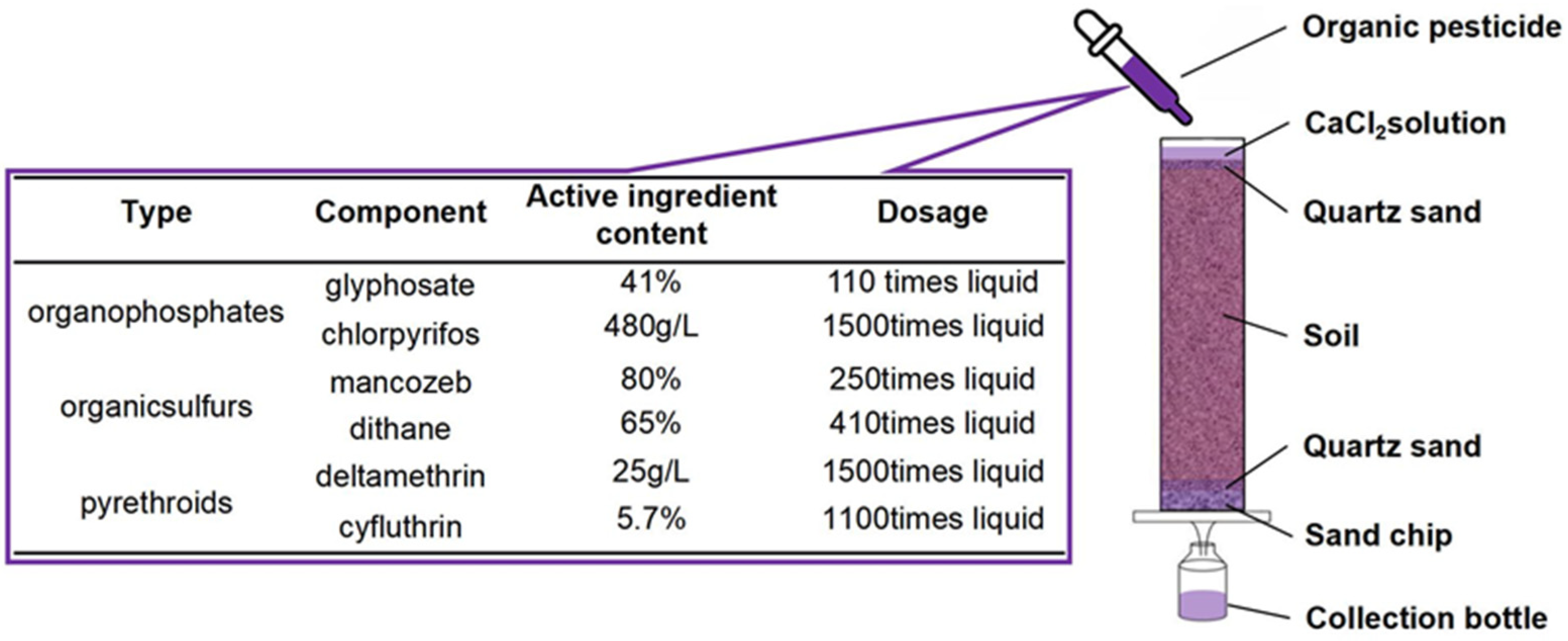
Figure 2.
(a) Streamline diagram of the vertical jet cylindrical chamber; (b) Streamline diagram of the vortex jet cylindrical chamber; (c) CFD simulation streamlines and velocity contour of the vortex jet cylindrical chamber; (d) Structural diagram of the vortex E-nose sampling chamber. (Green markings indicate adjustable parameters, red indicates fixed parameters).
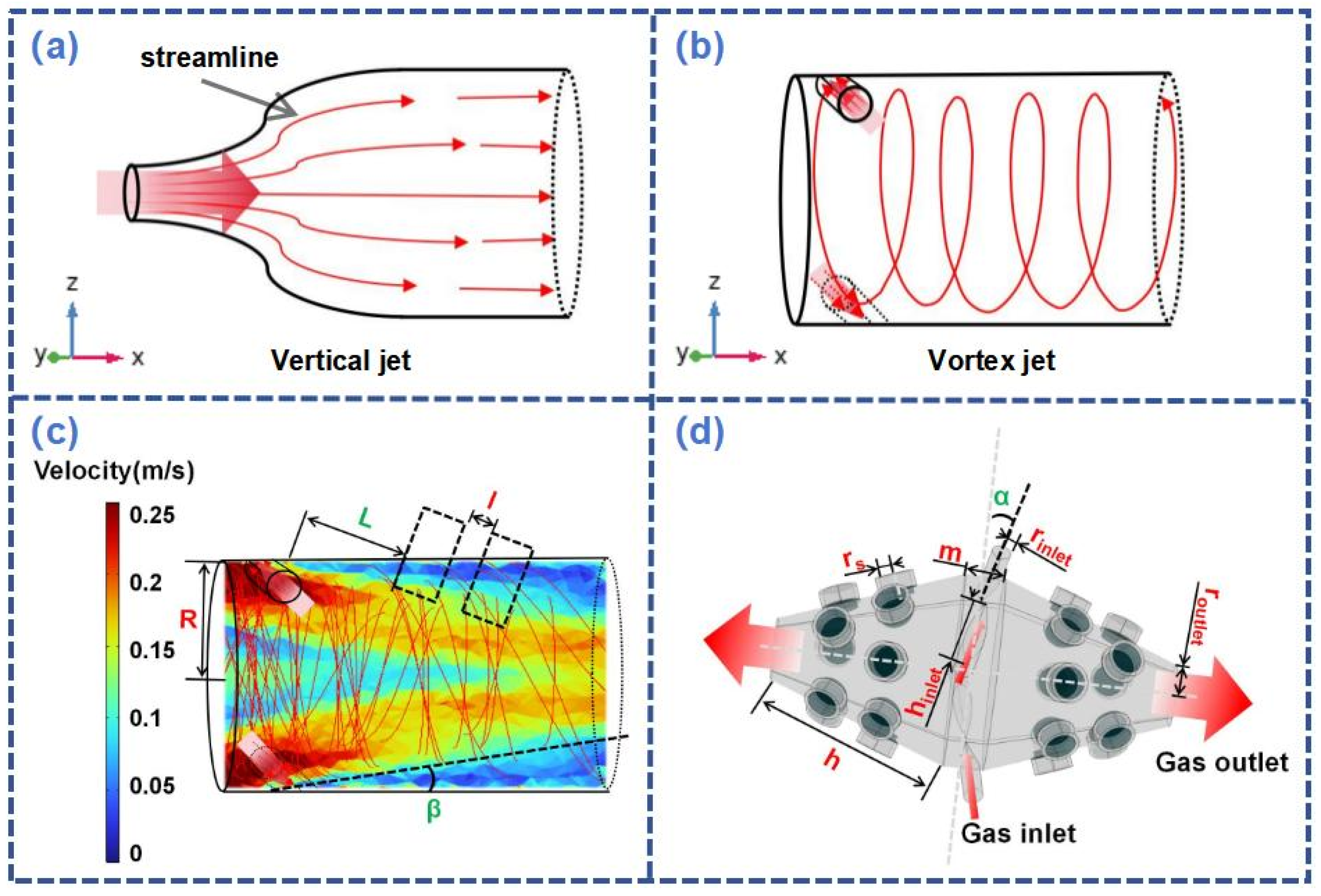
Figure 3.
Variation of and in different mesh numbers.
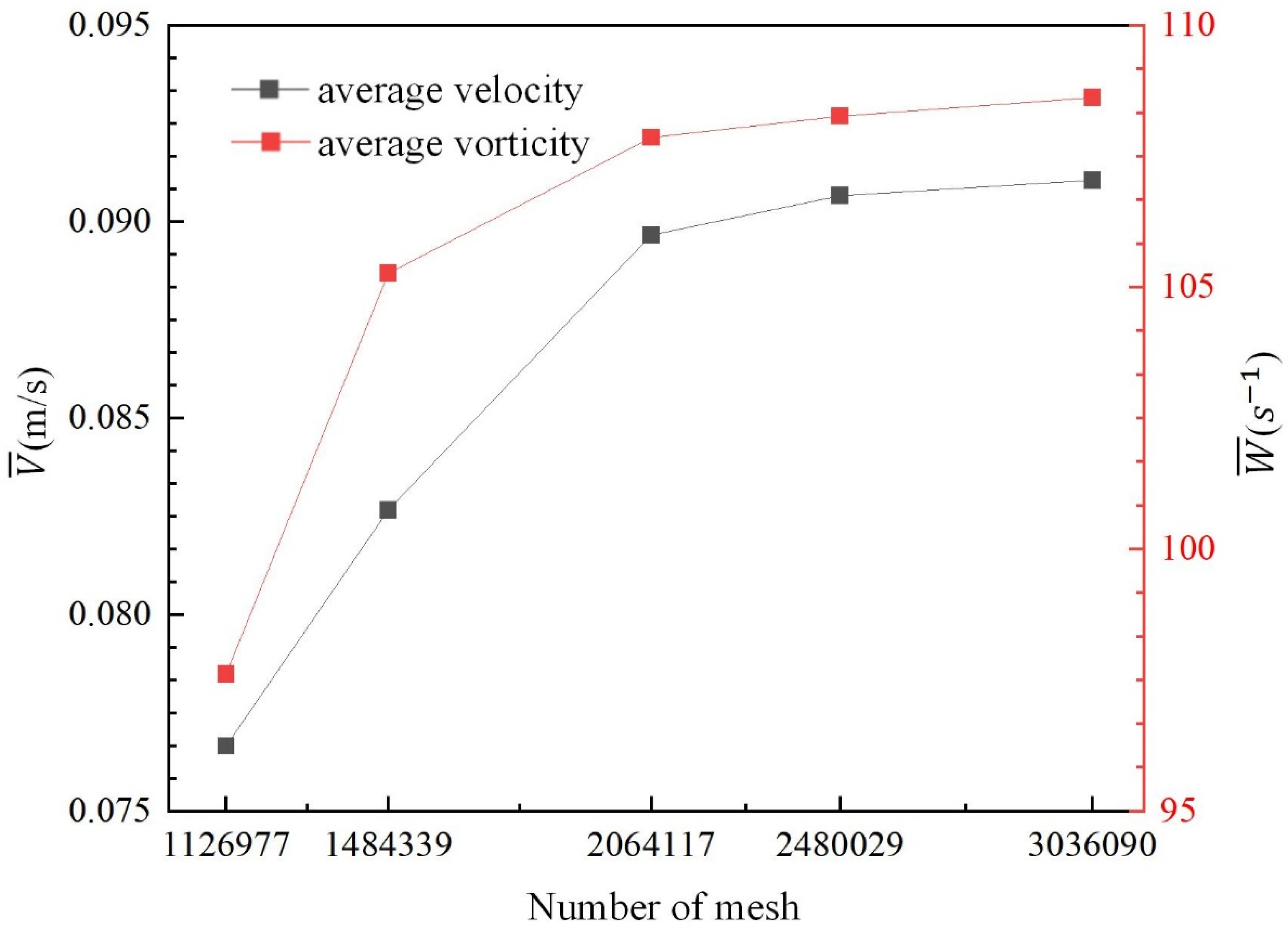
Figure 4.
Optimization process based on RSM and NSGA-II.
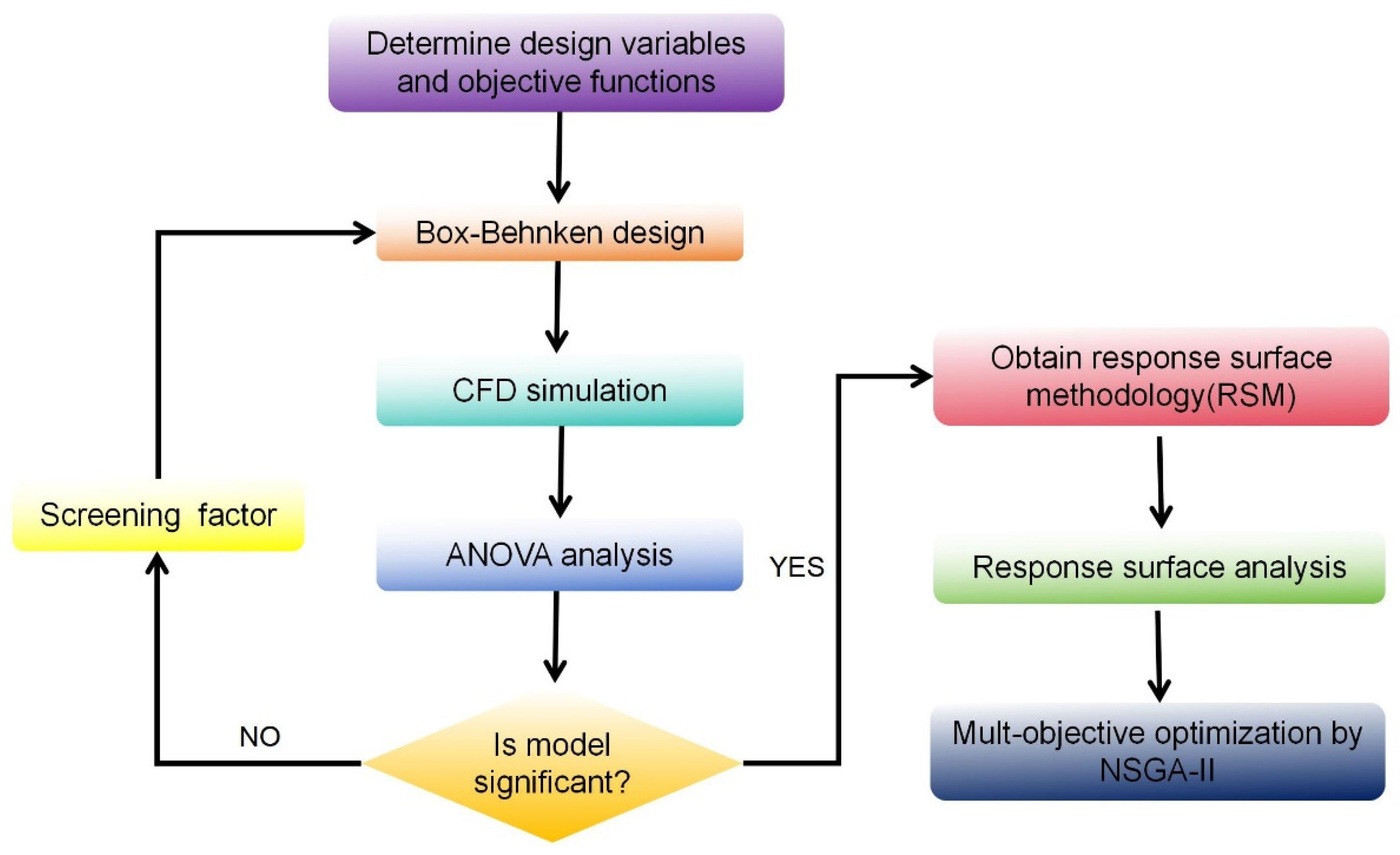
Figure 5.
Vortex E-nose for black soil pesticide identification.
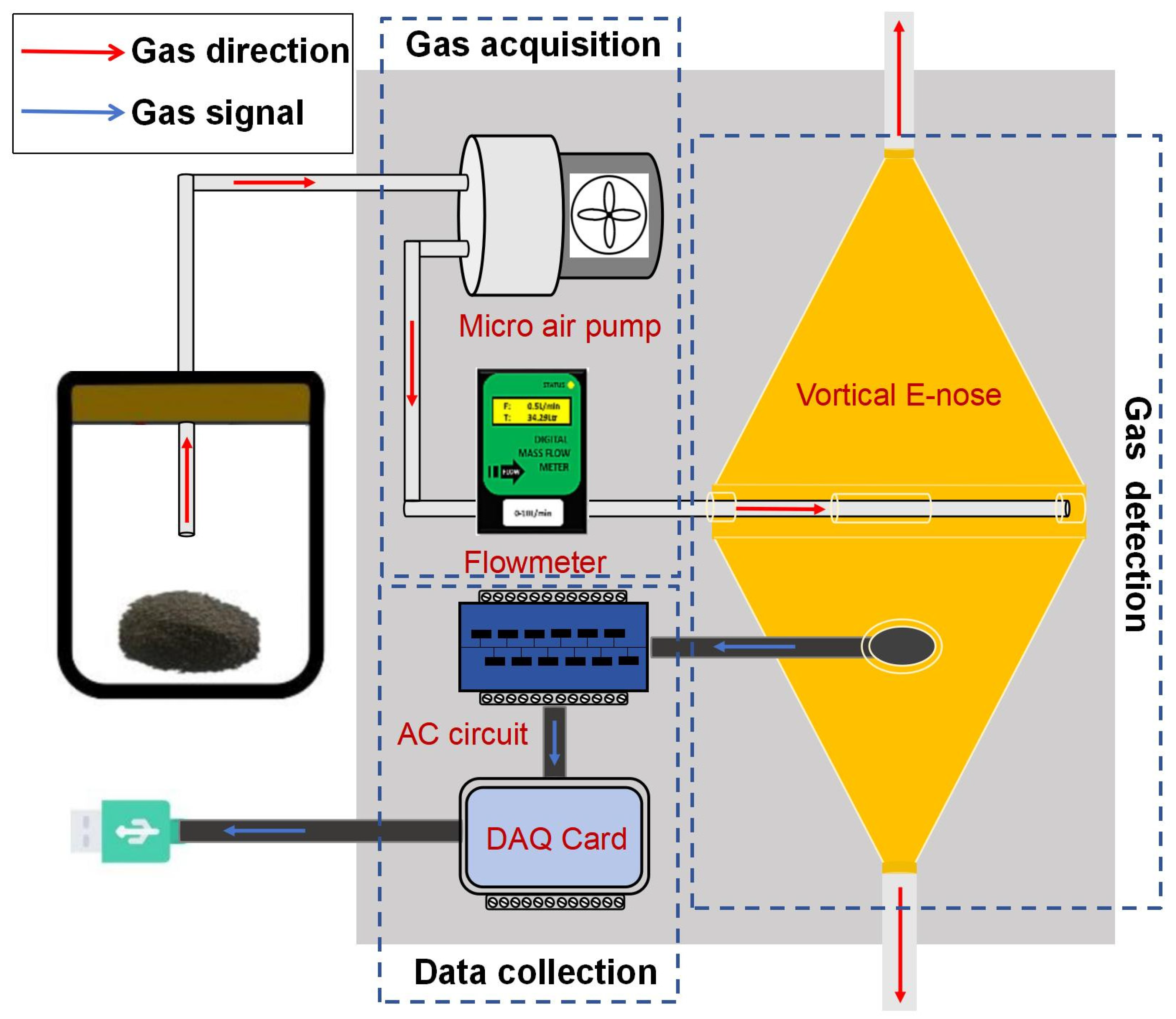
Figure 6.
3D response surface Analysis of and : (a) The impact of the interaction between β and Q on ; (b) The impact of the interaction between β and L on ; (c) The impact of the interaction between β and Q on ; (d) The impact of the interaction between Q and L on .
Figure 6.
3D response surface Analysis of and : (a) The impact of the interaction between β and Q on ; (b) The impact of the interaction between β and L on ; (c) The impact of the interaction between β and Q on ; (d) The impact of the interaction between Q and L on .
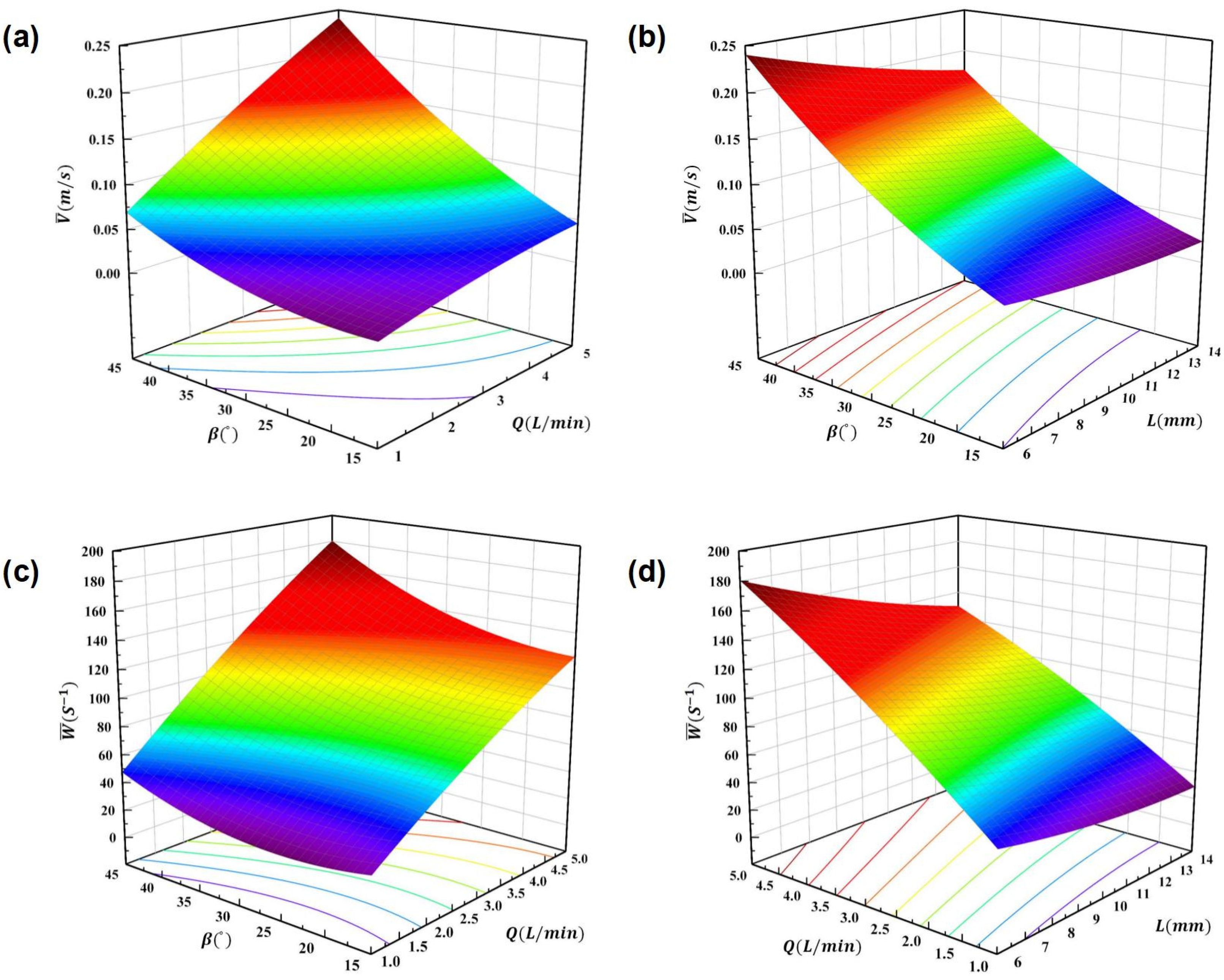
Figure 7.
Pareto-optimal points of multi-objective optimization.
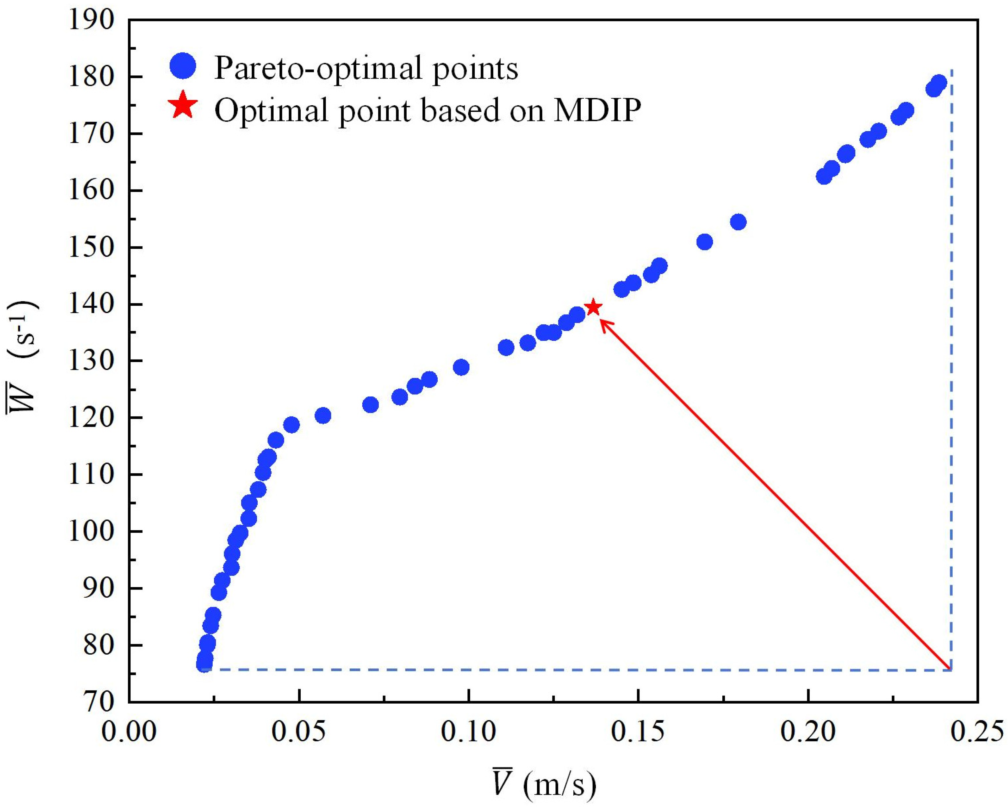
Figure 8.
CFD simulation results at the circumferential cross-section of the sensor near the inlet: (a) Velocity contour of the traditional vertical E-nose; (b) Vorticity contour of the traditional vertical E-nose; (c) Velocity contour of the vortex E-nose; (d) Vorticity contour of the vortex E-nose.
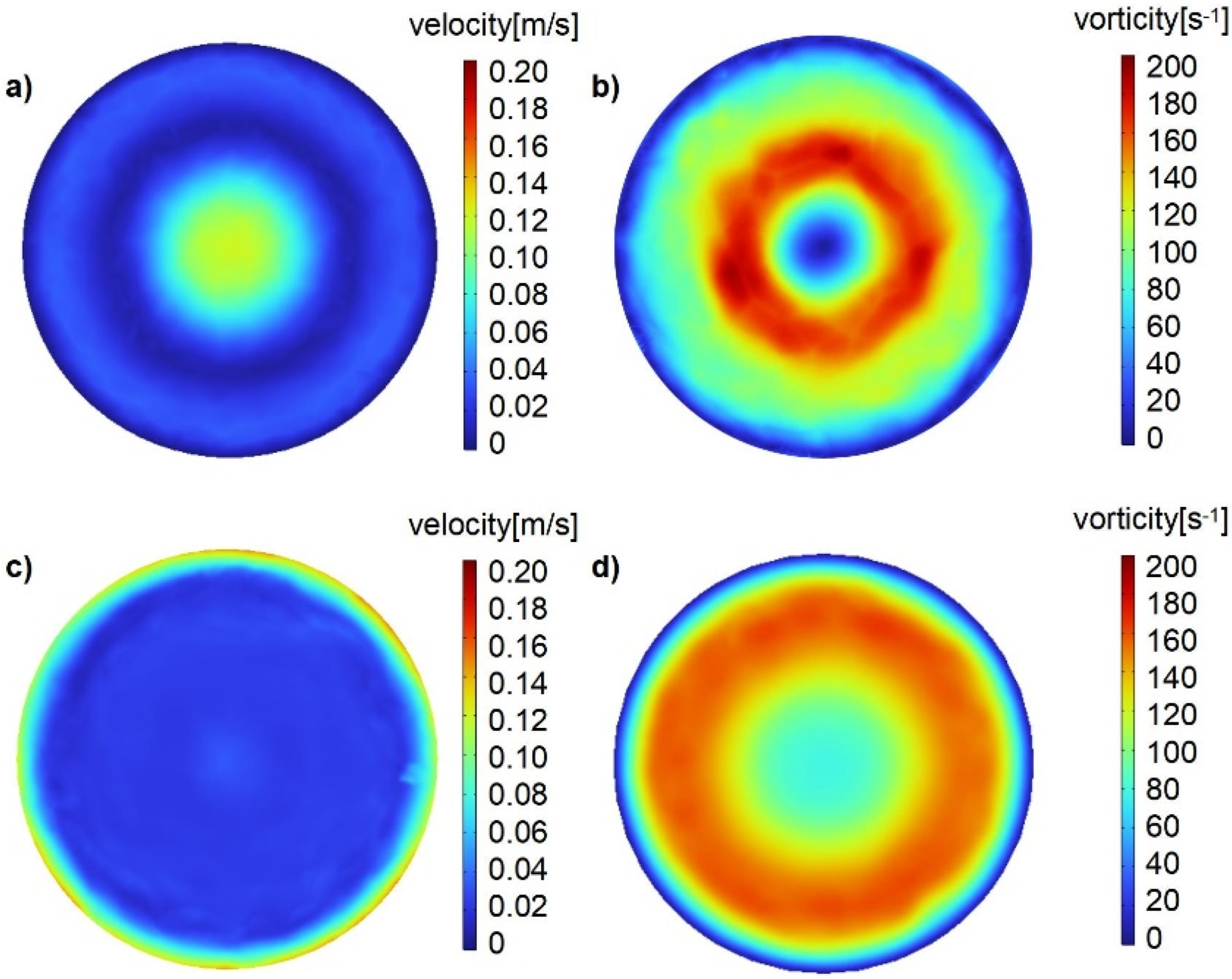
Figure 9.
Vortex E-nose sampling chamber:(a) modelling; (b) 3D printing.
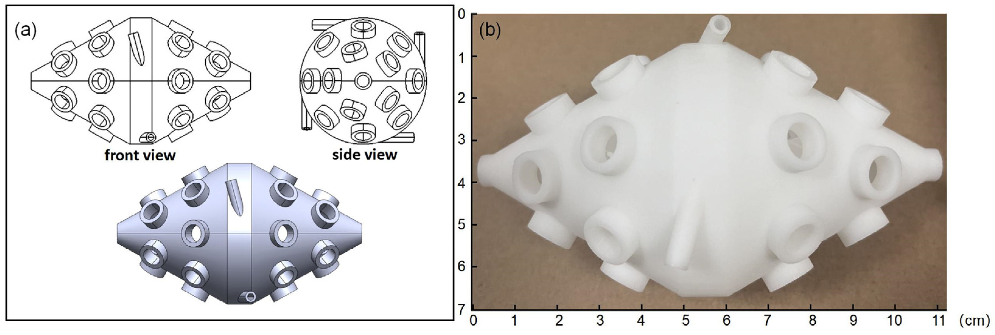
Figure 9.
ACC of vortex E-nose identification obtained through the confusion matrix: (a) Training set for organic pesticide types; (b) Test set for organic pesticide types; (c) Training set for organic pesticide components; (d) Test set for organic pesticide components.
Figure 9.
ACC of vortex E-nose identification obtained through the confusion matrix: (a) Training set for organic pesticide types; (b) Test set for organic pesticide types; (c) Training set for organic pesticide components; (d) Test set for organic pesticide components.
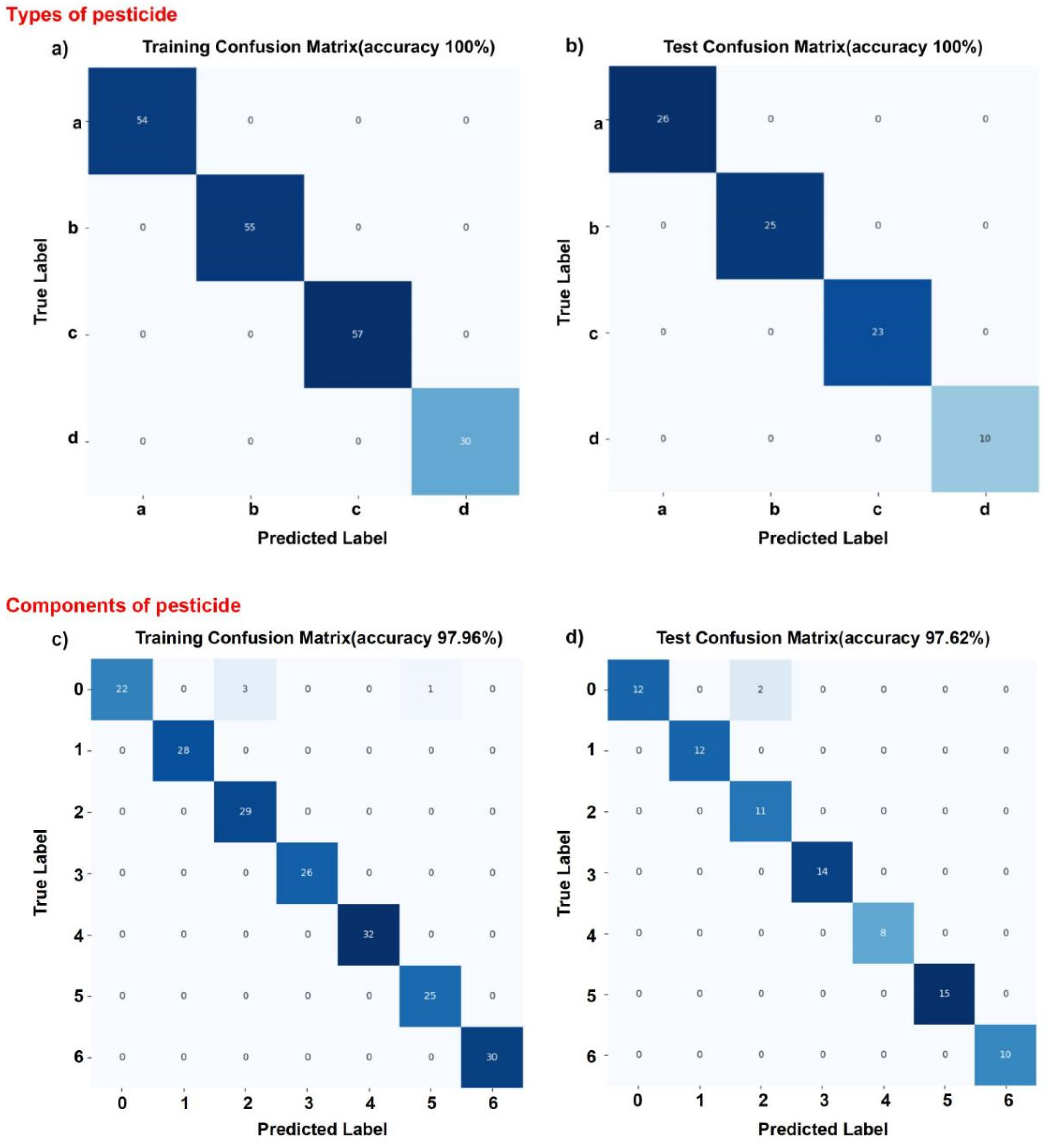

Table 1.
Levels of design variables.
| Design variables | Levels | ||
|---|---|---|---|
| α(°) | 0 | 20 | 40 |
| β(°) | 15 | 30 | 45 |
| Q(L/min) | 1 | 3 | 5 |
| L(mm) | 6 | 10 | 14 |
Table 2.
Response of BBD.
| Case | Variables | Response | ||||
|---|---|---|---|---|---|---|
| TestNo. | α(°) | β(°) | Q(L/min) | L(mm) | (m/s) | (/s) |
| 1 | 20 | 30 | 5 | 14 | 0.0725 | 82.4707 |
| 2 | 40 | 45 | 3 | 10 | 0.1336 | 100.0340 |
| 3 | 20 | 15 | 3 | 6 | 0.0291 | 73.0684 |
| 4 | 20 | 15 | 1 | 10 | 0.0052 | 13.5143 |
| 5 | 20 | 30 | 1 | 14 | 0.0089 | 10.4173 |
| 6 | 40 | 30 | 5 | 10 | 0.0942 | 106.3800 |
| 7 | 40 | 30 | 3 | 6 | 0.0750 | 84.4160 |
| 8 | 20 | 45 | 3 | 6 | 0.1573 | 113.0310 |
| 9 | 0 | 15 | 3 | 10 | 0.0237 | 59.4449 |
| 10 | 0 | 45 | 3 | 10 | 0.1033 | 76.2033 |
| 11 | 20 | 30 | 3 | 10 | 0.0521 | 59.2467 |
| 12 | 40 | 30 | 3 | 14 | 0.0476 | 54.2016 |
| 13 | 20 | 45 | 3 | 14 | 0.1028 | 74.7591 |
| 14 | 20 | 45 | 5 | 10 | 0.1900 | 139.5710 |
| 15 | 20 | 15 | 5 | 10 | 0.0380 | 95.3213 |
| 16 | 40 | 15 | 3 | 10 | 0.0296 | 73.9839 |
| 17 | 0 | 30 | 3 | 14 | 0.0417 | 47.2001 |
| 18 | 0 | 30 | 5 | 10 | 0.0827 | 93.8868 |
| 19 | 0 | 30 | 3 | 6 | 0.0680 | 78.0550 |
| 20 | 40 | 30 | 1 | 10 | 0.0144 | 16.8679 |
| 21 | 20 | 30 | 1 | 6 | 0.0167 | 19.8180 |
| 22 | 0 | 30 | 1 | 10 | 0.0112 | 13.1139 |
| 23 | 20 | 45 | 1 | 10 | 0.0218 | 17.0534 |
| 24 | 20 | 15 | 3 | 14 | 0.0184 | 46.5605 |
| 25 | 20 | 30 | 5 | 6 | 0.1097 | 124.5180 |
Table 3.
Sensor types and specific sensitive gas in vortex E-nose.
| Types | Specific sensitive gas (Near inlet) | Types | Specific sensitive gas (Near outlet) |
|---|---|---|---|
| MP-2 | C3H8, smoke | GSBT11 | VOCs |
| MP-3B | C2H5OH | MP801 | C6H6, CH2O, C7H8, C2H5OH |
| MP-4 | CH4 | MP901 | C2H5OH, CH2O, C7H8, C3H6O |
| MP-5 | LP gas | MP905 | C6H6, C7H8, C2H5OH, CH2O |
| MP-7 | CO | MS1100 | C6H6, C7H8, CH2O, |
| MP135 | H2, C2H5OH, CO | TGS2600 | C2H5OH, H2 |
| MP402 | CH4, biogas | TGS2602 | VOCs, H2S, NH3 |
| MP503 | C2H5OH, smoke, C4H10, CH2O | TGS2603 | Air pollutant |
| MP-702 | NH3 | WSP1110 | NO2 |
| MP-9 | CO, CH4 | WSP2110 | C6H6, C7H8, C2H5OH, CH2O |
| TGS2610 | LP gas | ||
| TGS2611 | CH4 | ||
| TGS2612 | CH4, C3H8, C4H10 | ||
| TGS2618 | C4H10, LP gas | ||
| TGS2620 | C2H5OH, organic solvents | ||
| WSP7110 | H2S, C2H2, CH2O |
Table 4.
ANOVA for and .
| Source | (m/s) | (s-1) | |||||
|---|---|---|---|---|---|---|---|
| Sum of squares | F | P | Sum of squares | F | P | ||
| Model | 0.0586 | 53.03 | <0.0001 | 32656.70 | 59.79 | <0.0001 | |
| α | 0.0003 | 4.30 | 0.0648 | 385.10 | 9.87 | 0.0105 | |
| β | 0.0266 | 336.75 | <0.0001 | 2100.36 | 53.83 | <0.0001 | |
| Q | 0.0216 | 273.50 | <0.0001 | 25333.43 | 649.32 | <0.0001 | |
| L | 0.0022 | 28.39 | 0.0003 | 2619.52 | 67.14 | <0.0001 | |
| αβ | 0.0001 | 1.89 | 0.1994 | 21.58 | 0.5532 | 0.4741 | |
| αQ | 0.0000 | 0.2142 | 0.6534 | 19.09 | 0.4894 | 0.5002 | |
| αL | 0.0000 | 0.0046 | 0.9470 | 0.1026 | 0.0026 | 0.9601 | |
| βQ | 0.0046 | 58.13 | <0.0001 | 414.34 | 10.62 | 0.0086 | |
| βL | 0.0005 | 6.08 | 0.0333 | 34.60 | 0.8868 | 0.3685 | |
| QL | 0.0002 | 2.73 | 0.1296 | 266.45 | 6.83 | 0.0259 | |
| 0.0000 | 0.1866 | 0.6749 | 36.69 | 0.9403 | 0.3551 | ||
| 0.0009 | 11.94 | 0.0062 | 510.73 | 13.09 | 0.0047 | ||
| 0.0001 | 0.9552 | 0.3515 | 77.89 | 2.00 | 0.1880 | ||
| 0.0001 | 0.9441 | 0.3541 | 49.70 | 1.27 | 0.2854 | ||
| 0.9867 | 0.9882 | ||||||
Disclaimer/Publisher’s Note: The statements, opinions and data contained in all publications are solely those of the individual author(s) and contributor(s) and not of MDPI and/or the editor(s). MDPI and/or the editor(s) disclaim responsibility for any injury to people or property resulting from any ideas, methods, instructions or products referred to in the content. |
© 2024 by the authors. Licensee MDPI, Basel, Switzerland. This article is an open access article distributed under the terms and conditions of the Creative Commons Attribution (CC BY) license (http://creativecommons.org/licenses/by/4.0/).
Copyright: This open access article is published under a Creative Commons CC BY 4.0 license, which permit the free download, distribution, and reuse, provided that the author and preprint are cited in any reuse.


