Submitted:
26 November 2024
Posted:
27 November 2024
You are already at the latest version
Abstract
This paper introduces a kinetic model that couples social behavior in crowds (such as social interpersonal distance or herding) with contagion dynamics. The approach is based on the so-called kinetic theory of active particles where the activity variable represents the psychological state of pedestrians as well as their state related to an infectious disease (e.g., susceptible, infected, etc.). The activity evolves as the crowd moves and eventually exits a closed room. Some case studies are proposed in order to demonstrate the role of activity and how contagion awareness and stress influence the crowd movement and its shaping behavior.
Keywords:
Kinetic theory
; Crowd dynamics
; Disease contagion
; Awareness (List three to ten pertinent keywords specific to the article
; yet reasonably common within the subject discipline
1. Introduction
The recent global health crises, such as the COVID-19 pandemic, have underscored the critical importance of understanding and modeling the dynamics of infectious disease spread in crowded environments. Traditional epidemiological models, while effective in many scenarios, often lack the spatial and behavioral granularity needed to accurately predict disease transmission in specific settings, such as during evacuations in indoor venues. For instance, contributions [1,2] provide some hints to understand spatial propagation of a disease. This paper builds upon the spatial kinetic model of crowd evacuation dynamics with infectious disease contagion proposed by Agnelli et al. [3] by introducing a novel variable that accounts for contagion awareness and its propagation among individuals in a crowd.
These methods have been extensively utilized to study large systems of multiple interacting living entities. Specifically, we refer to the kinetic theory of active particles (KTAP) as outlined in [4]. In this theory, interactions deviate from the classical mechanics of inert matter, as they do not conserve momentum and energy and are not reversible. This theory addresses the conceptual challenges of studying living matter. Unlike physical systems of inert matter, biological phenomena cannot be studied using the same foundational theories and causality principles. This distinction has been highlighted by scientists developing a mathematical theory of living systems, as in [5,6,7]. This theory has been successfully applied to biological fields such as cellular movement [8,9], immune competition [10] and disease propagation [11].
In addition, coupling crowd dynamics and disease propagation requires a multiscale approach due to the complex interactions at different levels [3,12,13]. At the microscopic scale, individual behaviors and interactions are modeled using ordinary differential equations, capturing the detailed dynamics of each person. At the macroscopic scale, the system is described by averaged quantities such as density and velocity, using conservation laws to model the overall flow of the crowd. The mesoscopic scale, which is the focus of the kinetic theory, bridges these two by describing the probability distribution of individuals’ states and incorporating nonlocal, nonlinear interactions through tools from statistical mechanics and game theory.
The transition from microscopic to macroscopic models can be understood through the framework of the Hilbert problem [14,15], which seeks to derive macroscopic equations from microscopic dynamics. This approach ensures that the macroscopic behavior of the system is consistent with the underlying microscopic interactions. By incorporating the contagion awareness variable into the kinetic model, we aim to capture the multiscale nature of crowd dynamics and disease spread, providing a comprehensive framework that can inform both theoretical studies and practical applications in public health and safety.
The original model by Agnelli et al. [3] integrates the movement of individuals within a bounded domain, considering interactions with the environment and among individuals as in [16], including the spread of an infectious disease. This model employs a kinetic theory approach, utilizing game theory to describe the decision-making processes of individuals as they navigate towards exits while avoiding high-density areas and potential infection sources. However, the model does not explicitly account for the role of contagion awareness, namely how individuals’ knowledge and perception of infection risk influence their behavior and, consequently, the overall dynamics of disease spread.
Incorporating contagion awareness into the model is crucial for several reasons. First, awareness can significantly alter individual behavior, leading to more cautious movement patterns and potentially reducing the overall infection rate. Second, the propagation of awareness itself can be dynamic, influenced by factors such as communication among individuals, visible symptoms, and public health messaging. By modeling these aspects, we can gain deeper insights into the interplay between human behavior and disease transmission, which is essential for designing effective intervention strategies. Some hints in this line of research can be found in the contribution by Quaini et. al. [17], where the authors present a model for the dynamics of human crowds where the spreading of an emotion (specifically fear) has an influence on the pedestrians’ behavior. More recently, papers [18,19] study how awareness and stress is spread using a macroscopic and a microscopic approach, respectively. The novelty of this present paper is the multiscale nature of the model: interactions are studied at the microscale, the model is mesoscopic and emerging macroscopic behaviors are obtained.
This paper extends the models by Agnelli et al. [3,16] by introducing a new microscopic variable describing contagion awareness, inspired by the framework described in [18,19]. This variable captures the level of awareness among individuals and its impact on their movement and interaction patterns. The extended model is tested through a series of simulations to explore various scenarios, including different levels of initial awareness, rates of awareness propagation, and their effects on evacuation efficiency and disease spread.
The structure of this paper is as follows: Section 2 presents the extended mathematical model, detailing the incorporation of the contagion awareness variable. Section 3 presents the numerical methods used for simulation and the setup of the case studies, as well as the results of the simulations, highlighting the impact of contagion awareness on crowd dynamics and disease transmission. Finally, Section 4 concludes the paper with a summary of findings and potential directions for future research.
2. The mathematical Model
This section derives the model coupling crowd movement within a bounded domain with disease contagion and awareness spread.
2.1. Functional Subsystems and Representation
Let be a bounded domain. Consider a large system of pedestrians, regarded as active particles, moving in . We assume that the domain has the following features:
- The boundary , including the exit zone . Note that E could be the finite union of disjoint sets, i.e., the domain may have several exit zones. For instance, in Figure 1 there are two exits and .
- The remaining of the boundary is an impenetrable wall , see Figure 1.
- For simplicity, the domain is assumed to be convex.
- The domain is characterized by a parameter that accounts for the quality of the environment, where represents the worst quality, forcing pedestrians to stop, and represents the best quality, allowing high speeds.
Remark 1.
Parameter α can be interpreted as an indicator of some features such as signaling, lighting, presence of obstacles or fire, etc. For more details, we refer to [16]. Even though the presence of internal obstacles is not included, it can be done through a straightforward technical generalization of the model, see [20].
To study the movement of pedestrians within the domain , let us introduce and describe their microscopic state. To do so, we consider the ideas presented in [16], where a representation with continuous-discrete hybrid features is defined. In the following, we detail the variables involved in our model:
- The position is assumed to be a continuous variable.
- For the velocity, denoted by in polar coordinates, it is assumed that the speed v is a continuous deterministic variable which evolves in time and space according to macroscopic effects determined by the overall dynamics, while the velocity direction is a discrete variable, heterogeneously distributed among pedestrians, attaining values in the setwith cardinal .
- A disease-related state given by a categorical variable in the set with cardinal . The set depends on the case under study. Two examples presented in [3] are with (each class S , E, I, and R corresponds to susceptible, exposed, infected, and recovered, respectively) and with (where V corresponds to a vaccinated class).
-
A state that represents a pedestrian’s level of awareness about the risk of contracting an infectious disease. We denote this variable by and define a discrete set of levelsThe lowest level corresponds to the state in which a pedestrian is not aware of a possible contagion (their only objective is to reach the exit). On the other hand, the highest level corresponds to the state in which a pedestrian is absolutely aware of a possible contagion and, therefore, their priority will be to avoid high densities. It is worth stressing that even in that case, pedestrians do not lose the objective of leaving the room.
Remark 2.
The term functional subsystem (FS) will be used to identify groups of particles sharing a common micro-state. For instance, the -FS refers to those active particles belonging to the -class, having a level of awareness and moving with direction . We can also (if the case under study requires it) represent functional subsystems for a micro-state concerning a single variable, e.g., -FS denotes those active particles who have a level of awareness .
The overall state of active particles is given by the distribution function . This is interpreted as the number of particles that, at time t, are located in , are carriers of the disease-related state and of a level of awareness and move with direction .
As in [3], the physical dimensions are removed by nondimensionalization, so that the maximum reachable local density is equal to 1 under normal conditions. In this way, the local density is given by the zero-th order moment:
Computing some marginal moments, let us obtain the local density of certain FSs. For instance, the local density of individuals belonging to the -class is
and the total population belonging to the -FS within the domain at time t is given by
2.2. Mathematical Structure
Following the models developed in [3,16], we take into account interactions of pedestrians with the environment and with all other pedestrians. For our large system of active particles that interact, subdivided into functional subsystems , the mathematical structure is obtained by a suitable balance of particles in the elementary volume of the microscopic states space. Therefore, the net flow into such volume is given by:
for , and , and where . The left-hand term models the transport of particles, while the right-hand side term represents the net balance for those particles in the -FS due to interactions.
In this study we assume that the interaction dynamics, represented by the nonlinear term in equation (2), are determined by the following features:
- 1.
- moving towards the exit;
- 2.
- avoiding collision with walls;
- 3.
- moving towards less congested areas;
- 4.
- attraction to follow the main stream;
- 5.
- disease contagion;
- 6.
-
pedestrian awareness.Note the distinction between the first two items, which are related to purely geometric characteristics of the domain, and the subsequent four, which take into consideration that pedestrian behavior is strongly affected by the presence of other pedestrians. Thus, we split the interaction term into two terms
Interactions can modify the internal state of the interacting pedestrians. Here, we assume that interactions between pedestrians and the environment (given by items 1 and 2) may modify the walking direction of the pedestrian. While interactions between pedestrians (related to items 3 to 6) can modify the walking direction of the pedestrian, but also can modify the disease-related state and the awareness level , see Figure 2 for a schematic representation (and Section 2.3 for a detailed description).
In order to model changes in the internal state we use probabilistic rules. Taking inspiration from [3], we define the following transition probabilities
- with models changes in the velocity direction. The quantity is the probability that an individual moving with direction , adjusts its direction into as a consequence of the domain geometry (e.g., walls or exit doors).
-
with , and models inter-pedestrian interactions. In this study, we assume three different types of interactions between pedestrians which are modeled by the following transition probabilities:
- *
- describe the probability that a -individual undergoes a transition into the disease state as a consequence of an interaction with a -individual,
- *
- represents the probability that an individual with level of awareness changes to level as a consequence of an interaction with an individual with level of awareness , and
- *
-
denotes is the probability that an individual moving with direction changes its direction into after an interaction with a pedestrian walking with direction . In Section 2.3.2 we will see that this transition also depends indirectly on the awareness level of the individual.Then, the compact form of inter-pedestrian interactions transition probability is given by the product
Remark 3.
Notice that the symbol represents transitions depending only on the geometry of the domain, while considers interactions among pedestrians.
The transition probabilities and satisfy
guaranteeing the conservation in the number of total pedestrians.
By considering the above-defined terms, Eq. (2) can be written as
for , and , where . The expressions and are the interaction rates modeling the frequency of interactions with the geometry of environment and with other pedestrians, respectively.
2.3. Modeling the Interactions
Let us now focus on the modeling of interactions that results in the specification of the right-hand side of equation (3). We differentiate two types of dynamics: (i) dynamics induce by the shape of the environment and (ii) dynamics induced by interactions between pedestrians. The first type is related to describe interactions between a pedestrian and the geometry of the domain where the dynamics occurs and this type of interactions can produce a change in the walking direction of the pedestrian. The second type of dynamics is associated with binary interactions between pedestrians. This type of interaction may produce a transition into the disease state, a change in the level of awareness and also change in the walking direction.
Before starting to describe the two types of dynamics mentioned previously, it is necessary to define three types of particles (pedestrians):
- test particles with micro-state which are representative of the whole system;
- field particles with micro-state , whose presence triggers the interactions of the candidate particles and;
- candidate particles with micro-state , which can reach in probability the state of the test particles after individual based interactions with field particles or with the environment.
2.3.1. Dynamics Induced by the Shape of the Environment.
Following the ideas presented in [16], we assume that the geometry of the domain has an influence on the pedestrian’s choice of his/her walking direction and this influence is due to:
- Trend to move toward the exit. During an evacuation, pedestrians may try to reach the exit by moving through the shortest path from their current location. Given a candidate particle at the point , we define its distance to the exit aswhere denotes the Euclidean norm in , and we consider the unitary vector , pointing from to the exit, see Figure 3(a).
- Trend to avoid the collision with walls. A pedestrian at position and moving in direction , that does not point towards the exit, will collide with the wall at a point and a distance from him/her, unless he/she changes direction, see Figure 3(b). Thus, to avoid this collision, the pedestrian must select a suitable new direction. Building on the model presented in [16], we define the unit tangent vector along the boundary at , oriented to guide the particle closer to the exit.
The two previous mentioned trends are related to purely geometric aspects of the domain, meaning that candidate particles take into account the presence of doors or walls. The modeling approach is based on the following assumptions:
- (A1)
- The trend to the exit increases as particles get closer to it.
- (A2)
- Particles are subject to a stronger influence to avoid the wall as they get closer to it.
Different pedestrians are not expected to react in the same way when facing a certain particular situation. That is, every pedestrian, depending on his/her position, has the ability to employ a different strategy to choose which direction to move, either avoiding the walls or reaching the exit. This heterogeneity can be efficiently modeled in a probabilistic manner. Specifically, to model the dynamics induce by the shape on the environment we consider the following two terms:
- The interaction rate , that models the frequency of interactions between candidate particles and the boundary of the domain. We suppose that decreases with local density, since the lower this quantity is, the easier is for pedestrians to realize about the presence of walls and doors. Following this idea, we assume .
- The transition probability is the probability that an h-candidate particle adjusts its direction into that of the test particle , induced by the presence of walls and exit areas.
The modeling approach assumes that pedestrians change direction, in probability, only to an adjacent (clockwise or anticlockwise) direction in the discrete set . This means that a candidate h-particle may eventually end up into the states , or remain in the state h. Notice that in the case we set , while in the case we set .
The set of all transition probabilities forms the so-called table of games that models the game played by active particles interacting with the geometry of the environment.
According to assumptions (A1)-(A2), we define the vector
whose direction is the geometrical preferred direction, meaning the ideal direction that a pedestrian should take in order to reach the exit and avoid the walls in an optimal way.
Since directions are discretized, an h-particle will update its direction by choosing among the three allowed outputs , and the closest to . The compact form of the table of games is given by
where
denotes the Kronecker delta function, and the coefficient , proportional to the parameter , is introduced to describe the fact that even in the case that the geometrical preferred direction is close to , a transition may occur, and the more distant the two states are, the more probable is this transition:
where . Notice that if , then and , meaning that a pedestrian keeps the same direction, at least due to the influence of the geometrical features, with probability 1.
2.3.2. Dynamics Induced by Interactions Between Pedestrians
Binary interactions, at each time t and position , involve test, candidate, and field particles. A candidate particle modifies its state, in probability, into that of the test particle, due to interactions with field particles, while the test one may lose its state as a result of these interactions. To model the dynamics induced by interaction between pedestrians we consider the following two terms:
- The interaction rate , that defines the number of binary encounters per unit time. If local density increases, then the interaction rate also increases.
- The transition probability , that represents the probability that a pedestrian with infectious state , level of awareness and moving with direction undergoes a transition into infectious state , level and direction after an interaction with a pedestrian with state , level of awareness and moving with direction .
Note that interaction between pedestrians can produce: (i) a transition into the disease state (ii) a change in the level of awareness of the particles involved and (iii) a change in the walking direction , which in turn is affected by the level of awareness. In the following, we will analyze each interaction and its outcome in detail.
(I) Interactions can modify the state related to the disease.
Each individual is carrier of an internal micro-state accounting for their condition related to an infectious disease. Let us first consider the simplest case in which the population is partitioned into four mutually exclusive compartments (that can be treated as well as functional subsystems in our theoretical framework). Specifically, let where S, E, I and R denote, respectively, susceptible, exposed, infectious and recovered hosts.
Note that since the time scale of interest for movement and evacuation from a room is too short compared to the period from time of infection to time of being contagious or infectious, it is imperative to include in our model the disease latency period and, thus, the exposed compartment E. When a susceptible individual interacts with an infectious one, she may get infected but -during the latency period- will not transmit the disease, until a transition from E to I takes place. This may occur for sure after the evacuation and we are interested in monitoring the dynamics of contagion during evacuation.
The dynamics of an SEIR model can be described by the following reaction scheme:
where permanent waning immunity is being assumed (thus, individuals belonging to the R compartment remain there).
Here, we assume that contagion occurs following the law of mass action, with infection rate at which a susceptible individual may become exposed after an interaction with an infected individual. The transitions from E to I and from I to R depend only on the compartment sizes, with and denoting the respective transition rates. However, since we are only interested in the evacuation time interval, our table of games shall only consider the first transition in Eq. (4). Thus, rates and can be neglected and the only non-trivial entry in the table of games for contagion dynamics takes the form , while all the other interactions do not undergo any kind of transition.
It is useful to include a vaccinated class, as will be considered in the numerical experiments afterwards. To do so, we simply add a compartment V including susceptible individuals that can get infected but with a lower infection rate. In the case of a perfect sterilizing vaccine, the infection rate would be 0 but in general we shall assume a non-negative value .
The reaction scheme for the so-called SEIRV model is:
and the transition probability densities shall be changed accordingly by adding the non trivial entry .
(II) Interactions can modify the level of awareness.
We assume that a binary interaction between pedestrians can modify their awareness level. More in detail, let us consider the different kinds of interactions that can occur between a candidate pedestrian with awareness level and a field pedestrian with awareness level :
- If two pedestrians with the same awareness level interact, then both of them remain at the same level.
- If two pedestrians with different levels of awareness interact, then one pedestrian can influence the other and, as a result, the pedestrian having a lower awareness level may increase her level, while the one with a higher level may face a decrease in her level of awareness.
Notice that an individual with awareness level cannot decrease her level since she is at the lowest possible level. Similarly, an individual with awareness level cannot increase her level which is already at the highest possible stage. Therefore, after an interaction between a candidate particle with awareness level and a field particle with awareness level the possible levels to which the candidate particle can change are given by the following set of indices
Taking all the previous assumptions into account, the transition probability is given by
where m is defined as
is given by
and where is a parameter related to the influence between pedestrians. A larger value indicates a greater probability of changing state , meaning the candidate particle is largely influenced by a field particle. Conversely, a lower value leads to a reduced probability, meaning that the candidate particle is not much influenced by a field particle.
(III) Interactions can modify the walking direction.
Following the model presented in [16], we assume that pedestrians, induced by interaction with other pedestrians, may decide to change their walking direction taking into account the combination of the following causes:
- Tendency to move towards less congested areas. In order to facilitate its movement, a candidate pedestrian at , moving with direction , may decide, under the influence of his/her level of awareness , to change direction by moving towards less congested areas. This direction is denoted by the unitary vector and can be computed by choosing the direction that gives the minimal directional derivative of the density at the point .
- Tendency to follow the stream. A candidate pedestrian, moving with direction and level of awareness , that interact with a field pedestrian may decide to follow him/her and in consequence adopt a new velocity direction. We define the unitary vector to describe the movement of the field particle moving with direction .
We observe that the two tendencies take into account that pedestrian behavior is affected by that of the others. In fact, on the one hand, a candidate pedestrian is capable of scanning its surroundings in order to choose, at each moment and position, a proper direction that will prevent it to move into congested areas, while on the other hand, the interaction with a field pedestrian will try to bring its direction closer to that of the latter.
Moreover, the two previous tendencies compete with each other. In other words, higher densities will induce a higher tendency to look for less congested areas but at the same time to follow the stream. In fact, in [16] authors introduce a parameter that reinforces one tendency or the other according to the particular situation to be modeled. The value corresponds to the situation in which only the research of less congested areas is considered, while corresponds to the situation in which only the tendency to follow the stream is taken into account.
In this study, we propose a different approach and assume that the two tendencies are also related to the level of awareness of each pedestrian. Specifically, we assume that the higher the level of awareness of a candidate particle, the greater the probability of selecting a proper direction towards less congested areas. Conversely, lower the level of awareness of a candidate particle, greater the probability of following the stream. Therefore, differently from [3,16] where all pedestrians adopt the same strategy to follow the stream or to search for less congested areas, in this study we define a decreasing function , which will make every pedestrian in the -FS have their own parameter depending on its level of awareness.
Therefore, our modeling approach is based on the following assumptions:
- (A3)
- The tendency to look for less congested areas depends on the local density and level of awareness of each active particle.
- (A4)
- The tendency to follow the stream depends on the local density and level of awareness of each active particle.
Next, based on assumptions (A3) and (A4), we present how the transition probability .
On the one hand, in order to change direction to move towards less congested areas we consider how pedestrians react according to their perception of the density around them and choose the less congested direction among the three admissible ones. This direction can be computed for a candidate h-pedestrian in position by taking
where denotes the derivative of in the direction . In this way, we have . Notice that in the case we set , while in the case we set
On the other hand, recall that denote the vector pointing in the direction of the field particle.
Then, according to assumptions (A3)-(A4), we define the vector
where the subscript P stands for pedestrians, and the direction of is the interaction-based preferred direction, obtained as a weighted combination between the trend to follow the stream and the tendency to avoid crowded zones, under the influence of awareness level . Then, we propose the following table of games:
where n is defined as
and is given by
Remark 4.
Notice that the superscript p is implicit in the definition of since it impacts on the definition of the interaction preferred direction .
2.4. Modeling the Velocity Modulus
The variation in pedestrian velocity is influenced by interactions among individuals. Pedestrians adjust their walking speed according to how crowded their surroundings are. We assume that the maximal reachable dimensionless velocity modulus depends linearly on the quality of the environment, in such a way that –any movement is hindered– and –maximal speed is attainable when the environment is ideal. Additionally, we assume that speed velocity is influenced by locally perceived density. Specifically, the maximum velocity is maintained under low-density conditions (free-flow regime) until a critical density is reached, which can be experimentally measured. When the locally perceived density exceeds this threshold, the velocity modulus decreases to zero (slowdown zone). Within this zone, we choose a polynomial-type dependence of the velocity modulus on the local density. We refer to Sec. 2.3 of [16] for more details.
3. Numerical Results and Cases of Study
In this section, we present a set of numerical simulations of the model (2) in which we explore and analyze the performance of the proposed model in different scenarios.
In order to solve numerically equation (2), we must explicitly define initial conditions , for , and , while boundary conditions are not explicitly imposed but are induced by the non-local action over the pedestrians given by the term . Indeed, pedestrians are induced to avoid walls according to the trends described in Section 2.3.1. To obtain a numerical solution of the system (2), we use a splitting method [21], where the overall evolution operator is seen as the sum of evolution operators for each term in the model. Then, each term is solved by means of an appropriate scheme, and finally all the pieces are attached together. In particular, Eq. (2) is split into two sub-equations:
and
for and . Note that equation (7) is a 2D homogeneous transport equation. Hence, to guarantee conservation of the total number of particles, we use a finite volume scheme to solve it. We refer to [22,23,24] for more details on the implementation. On the other hand, Eq. (8) is solved by means of a first order Euler explicit method to go forward in time.
In all the numerical experiments of this section we consider a square domain of side length 10 m with an exit door of width 2 m located on the right. This is the same domain used in [3,16,20]. The quality of the environment, , is fixed for all case studies. We choose so that each pedestrian has the possibility to reach her maximum permitted speed. Similarly, interactions rates are fixed and equal to and . Additionally, we deal with nondimensional quantities obtained by referring to the spatial coordinates relative to the longest dimension of the domain m, while density and velocity modulus are referred to and m/s, respectively, following the experimental values presented in [25]. From these values, we obtain the reference time s. The set related to the disease state is given by
Infection rates and are kept fixed. Note that contagion is considered only within the domain as we do not monitor disease dynamics once individuals are outside the room. Additionally, the set related to the awareness level is defined as
and parameter in equation (5) related to the influence between pedestrians is fixed, we choose . Finally, the set of possible velocity directions is given by
while the velocity modulus is assumed to depend on the perceived density and on the quality of the environment. In all the considered case studies we assume that approximately 50 pedestrians are initially moving with direction . Thus, , for , and .
Recall that, according to equation (1), the total number of pedestrians belonging to each infectious compartment within the domain and at time t is given by
where , , and are the susceptible, exposed, infectious and recovered populations within the domain, respectively. Note that contagion is considered only within the domain as we do not monitor disease dynamics once individuals are outside the room.
Similarly, the total number of pedestrians with awareness level within the domain and at time t is given by
In the following subsections, we present a selection of case studies aimed to understand and analyze the model performance under different scenarios. The first case study focuses on the influence of awareness levels on the overall dynamics. In the second case study, we attempt to determine which condition, aware or vaccinated, preponderates in leading to fewer infections. Finally, we study different functions involved in the definition of the interaction-based preferred direction (6).
3.1. Case Study 1: The Influence of Awareness Levels
In this case study we analyze the influence of the state on the evacuation process. Our objective is to understand how this state affects pedestrian behavior and its subsequent consequences on the spread of infectious diseases and evacuation times. Furthermore, we investigate whether has an indirect influence on velocity magnitude. For this first case study, we choose eight different scenarios to examine. Table 1 presents the different scenarios that are studied, showing the initial proportions of the involved populations related both to awareness and infectious levels. In addition, the last column shows the definition of function that is used for each scenario, that for this case study is maintained as .
Let us first analyze the influence of awareness levels on pedestrians. We observe in Figure 4 that scenarios where a large percentage of pedestrians initially have the highest awareness level lead to fewer exposed individuals compared to scenarios that started with a large percentage at the level . First, we focus on scenarios where most of the population initiates at level , these are scenarios 2, 4 and 6. Pedestrians with an awareness level consider the strategy of moving towards less crowded areas to avoid possible contagion, while still aiming to exit the room. Therefore, when more pedestrians apply this strategy, they have fewer chances of becoming exposed: this is exactly what happens in scenarios 2, 4, and 6. Conversely, scenarios with a majority of pedestrians that begin at level , that is scenarios 1, 3 and 5, lead to an opposite situation. Since pedestrians with awareness level focus on finding the exit rather than avoiding densely populated areas, they become more vulnerable to contagion. Figure 4 demonstrates that this strategy significantly increase their chances of becoming exposed. Finally, we analyze scenarios 7 and 8, where of pedestrians are initially equally distributed in the central awareness levels and . In scenario 7, the remaining pedestrians are divided between at awareness level and at awarness level . In contrast, scenario 8 initially has of pedestrian at level and at level . Notably, despite the similar initial distributions, the results observed are similar to those in previous scenarios, reinforcing the finding that a higher percentage of pedestrians starting at the highest awareness level results in fewer exposed individuals and shorter evacuation time.
Figure 4 also illustrates the impact of awareness level on evacuation time. Observe that scenario 6 (where all pedestrians have level ) achieves the shortest evacuation time, whereas scenario 5 (where all pedestrians have level ) results in the longest evacuation time. This difference is due to the opposite behavior tendencies. Pedestrians with level prioritize reaching the exit over avoiding congestion, leading to crowding and forced to stop. In contrast, pedestrians with level actively seek less congested areas and maintain distance from others, allowing continuous movement. Figure 5 shows these contrasting behaviors during the evacuation process.
To better understand the difference in the evacuation times, we examine how the proportions of the different awareness levels change with respect to time for each scenario. Recall that the total number of pedestrians with a given level of awareness level at time t is given by (9). Figure 6 presents the results, revealing two key trends: (i) a symmetric pattern emerges between opposing scenarios, and (ii) a tendency towards intermediate awareness levels occurs. Specifically, scenario 1 starts with an initial high proportion of pedestrians in level , but interactions among pedestrians during evacuation process lead to a pronounced transition towards level , see Figure 6 (a). Similarly, scenario 2, where most pedestrians initially belong to exhibits a similar trend with interactions that drive pedestrians to the level , see Figure 6 (b). The same kind of behavior can be observed /Similar trends are observed in scenarios 3 and 4 (Figure 6 (c) and (d)) and scenarios 7 and 8 (Figure 6 (g) and (h)). We understand that these tendencies towards the central levels occur because of the way in which the tables of games are defined. As discussed in Section 2.3, when pedestrians with different levels interact, there is a positive probability of moving closer by one level, but cannot move further apart, resulting in a natural convergence towards central levels. Regarding scenarios 5 and 6, no evolution in awareness levels is observed, see Figure 6 (e) and (f), respectively. This happens because the entire population belongs to a single level, so when pedestrians interact with others of the same level, the probability of staying in the same state is always 1 indicating no possibility of changing awareness levels.
Finally, Figure 7 shows the evolution of the minimum velocity reached by pedestrians with respect to time for all the proposed scenarios. It can be seen that there is an indirect influence of awareness levels on the velocity modulus of pedestrians. In scenarios 1, 3, and 5 (Figure 7 (a), (b) and (c)), pedestrians (at least one) reach a minimum velocity of zero during almost the entire evacuation process. This phenomenon is interesting because if there was at least one pedestrian with zero velocity throughout the evacuation process, it means that at almost any time, at least one pedestrian had to stop due to the high density generated by congestion. This congestion is a consequence of the strategy of pedestrians to follow the main stream, heavily influenced by the level , leading to overcrowding. Recall that these scenarios start with a vast majority proportion of individuals at awareness level .
On the other hand, in scenarios 2, 4, and 6 (see Figure 7 (a), (b) and (c)), the minimum velocity of pedestrians does not reach zero during the evacuation process. This indicates that pedestrians maintained movement throughout the evacuation, avoiding stops. These scenarios start with a vast majority proportion of individuals at awareness level . The underlying strategy of avoiding high congested areas, strongly influence by level , enabled pedestrians to create and exploit low-crowding zones. By doing so, they were able to continue walking without interruptions, demonstrating the effectiveness of this strategy in preventing congestion.
Figure 7 (d) presents the results of intermediate scenarios 7 and 8. It is worth noticing that both scenarios exhibit time intervals in which the velocity of pedestrians (at least of one) drops to zero. However, a comparison of the minimum velocities achieved reveals a significant difference: scenario 8, with of pedestrians starting at awareness level always achieves a higher minimum velocity than scenario 7, where begin at level . This difference reinforces the influence of awareness level on velocity modulus.
Based on the previous results, we conclude that the awareness level has a profound impact on the evacuation process. Initially, we observed a significant influence on the spread of disease. However, as we explored various scenarios, we also noted considerable effects on other factors, including evacuation time and velocity modulus. The incorporation of awareness levels is a valuable contribution to our model, as it provides a better representation of pedestrians’ behavior and differentiates their strategies. Furthermore, this addition brings our model closer to simulating real-life situations.
3.2. Case Study 2: Awareness vs. Vaccination
In this case study we compare and contrast (i) a population that is aware to contagion vs. (ii) a vaccinated population. The main question to answer is: which microscopic state is the most effective in preventing massive spread: a high level of awareness or being vaccinated? From this question, other points of interest arise, such as studying combinations of different populations, for example, a proportion of the population that is vaccinated but not aware, or determining which distribution of initial proportions results in the lowest number of exposed individuals. Table 2 shows the scenarios to be studied with their respective initial involved populations as well as the definition of function . We consider various initial proportions for susceptible S and vaccinated V pedestrians for the different scenarios. However, in all scenarios of the pedestrians initially belong to the infectious compartment I. This choice aims to maximize the potential for disease contagion, enabling us to assess which state is more resilient against the spread of disease.
Results for the scenarios proposed in Table 2 are shown in Figure 8. We obtained some very interesting results. Let us start with scenario 9, which performs the worst, as it shows the highest increase in the total number of exposed pedestrians at the end of the evacuation process and the largest decrease in the proportion of susceptible and vaccinated individuals, as shown in Figure 8 (a) and (b), respectively. The observed differences can be attributed to the initial population composition, characterized by a majority of pedestrians with awareness level and with a higher proportion of susceptible (but non vaccinated) individuals compared to vaccinated ones. Conversely, scenario 14 presents a majority of individuals starting at awareness level and with a higher proportion of vaccinated individuals compared to susceptible (and non vaccinated) ones. Moreover, a point to note is that the final proportion of the exposed individuals does not exceed of the total population for this scenario. These two scenarios represent the extreme cases, producing outcomes consistent with predictions.
Let us move on to understand the combined scenarios. Scenario 10 has an initial population with a lower proportion of vaccinated individuals but a higher proportion of pedestrians start at level . However, this scenario presents a higher number of contagion compared to scenario 13 which has an initial proportion with a majority of individuals vaccinated and with awareness level . The comparison between these two scenarios is important as it provides an initial answer to our main question: being vaccinated seems to be more effective than having a high awareness level in preventing the spread of a disease. We can reinforce this assertion by comparing scenarios 12 and 13, as the same pattern occurs: a higher proportion of vaccinated individuals results in a lower number of exposed individuals, even when most people initially belong to level . It should be noted that the difference in the total number of pedestrians exposed at the end of the evacuation process between scenarios 12 and 13 is considerably smaller than that between scenarios 10 and 13.
An interesting comparison is between scenarios 10 and 11. As shown in Figure 8(a) the curve describing the evolution of the total number of exposed pedestrians over time intersect for scenarios 10 and 11. The same happens for the curve representing the evolution of the total number of vaccinated and susceptible pedestrians, see Figure 8(b). Recall that scenario 11 has the same initial number of vaccinated and susceptible (but non vaccinated) population and a majority of pedestrian starting at level . While scenario 10 has an initial population with a lower proportion of vaccinated compared to susceptible (and non vaccinated) pedestrians and a majority of individuals starting level . Note that the curves in Figure 8(a) and Figure 8(b) intersect at approximately 17 seconds. This intersection occurs because pedestrians are nearing the exit at that moment, generating a bottleneck (Figure 9). Pedestrians with awareness level or tend to crowd near the exit causing an increase in contagion of the infectious disease, as observed in scenario 11. In contrast, pedestrians with awareness level or choose to distance themselves when approaching to the exit, allowing a more fluid exit and reducing the number of infections, as seen in scenario 10.
According to the obtained results, we can say that conditions of being vaccinated and having a high level of awareness are both important to help prevent the spread of a disease, but in the case of an evacuation from a closed domain through a narrow exit, the condition of being vaccinated seems to be more relevant.
3.3. Case Study 3: Analyzing the Role of
In this last case study we focus on understanding the role of the function and its influence on the evacuation process. Recall that the values of this function reinforce the tendency to move towards less congested areas or in contrast reinforce the tendency to follow the stream, see equation (6). We would like to know how the different choices of affect or have an effect on the evacuation time and the spread of a disease. Table 3 shows the nine scenarios to be studied.
First, we analyze scenarios 15, 16 and 17 that end with the highest number of exposed individuals and longest evacuation times, see Figure 10(a). We attribute this to the fact that in these scenarios the majority of the initial population belongs to the awareness level and therefore, at least during the start of the evacuation, most pedestrians tend to follow the stream since is equal to 1 (for all considered functions ). This behavior causes high congestion, facilitating contagion and also increasing the evacuation time. Furthermore, as the evacuation progresses, some pedestrians initially at awareness level transition to levels or (the vast majority will transition to ). For these individuals, the values of the different functions differ. Specifically, the cubic function yields values closer to 1 at levels or compared to the quadratic and linear function. Consequently, pedestrians with awareness levels and have a stronger tendency to follow the stream when using the cubic function, whereas the linear function induce a weaker inclination to follow this behavior. This explain why, despite starting with the same initial population, scenarios 15, 16 and 17 end with difference in the evacuation time and in the total number of exposed individuals.
Next, we focus on scenarios 18, 19 and 20 that exhibit the most favorable outcomes, with the lowest number of exposed individuals and shortest evacuation times, see Figure 10(a). It is worth noticing, that the differences in evacuation time and final exposed pedestrians between these scenarios are less pronounced compared to the previous three. Specifically, scenarios 19 and 20 yield nearly identical results. This can be attributed to the majority of pedestrians starting at awareness level and for this level the values of all functions are equal. As time progresses, pedestrians transition to levels and , mainly to . Although the values of the different functions in are different, they are all in the range (see Figure 10(b)) and according to what was analyzed in [16], results in similar evacuation times (at least for a number of pedestrians like the one in this Case Study). In contrast, the values of the different functions in are in the range (see Figure 10(b)), and according to what was analyzed in [16] this has a huge impact on evacuation time, which reinforces the observed in the first three scenarios analyzed (scenarios 15, 16 and 17).
Finally, we examine scenarios 21, 22 and 23 to further understand the influence of function on the evacuation process. Recall that these scenarios assume initial proportions of pedestrians are evenly distributed across the levels of awareness. In Figure 10 we can observe that scenario 23 is the one with highest number of exposed individuals and longest evacuation times, while scenario 21 is is the one with lowest number of exposed individuals and shortest evacuation time, between this three. This result can be attributed to the fact the cubic function reinforce the tendency that pedestrians follow the stream.
Based on the previous results, we conclude that when the function takes values close to 1 at awareness levels , it significantly increases the tendency for individuals to follow the stream, leading to congestion and an environment favorable to spread of the contagious disease. In contrast, when values fall within the range , the influence to follow the crowd decreases, resulting in a more fluid evacuation process.
4. Discussion and Conclusions
This study presents an extended kinetic model to analyze the dynamics of social crowds in the presence of an infectious disease, incorporating a novel variable for contagion awareness. Through three case studies, we explored the impact of awareness levels on evacuation times and the spread of contagion. Our findings highlight several key points:
- Impact of awareness on disease spread: High levels of awareness significantly reduce the spread of disease. Individuals with high awareness adhere to social distancing, exhibit caution for themselves and others, and possess knowledge about safety and prevention measures. Conversely, low levels of awareness lead to greater disease propagation due to neglect of social distancing, indifference, and lack of knowledge.
- Awareness evolution: Pedestrians cannot independently evolve their awareness levels. In our model, the only way to transition to a different awareness state is through interactions with other pedestrians. This aligns with the findings of Kim and Quaini [17], who modeled emotional states (specifically fear) as continuous variables evolving over time. Unlike their model, where fear levels can change even if the entire population starts with the same level, our model shows that a population with uniform awareness levels remains static.
- Impact of awareness on the evacuation dynamics: Unexpectedly, we found that evacuation times were shorter for scenarios with high awareness levels. Initially, we hypothesized that low-awareness pedestrians, focused solely on exiting the room, would achieve faster evacuation by reaching their maximum allowed speed. However, high-awareness pedestrians, by maintaining social distance, actually evacuated more efficiently. This counterintuitive result is explained by the function , which influences evacuation dynamics. Our results are consistent with Agnelli et al. [16], who found that an optimal parameter value of minimized evacuation time. In our study, low-awareness pedestrians had values close to 1, while high-awareness pedestrians had values near 0. There are some practical applications to this counterintuitive result. For instance, during the COVID-19 crisis some airlines have implemented a system to deplane by rows to prevent contagion, resulting also in shorter disembarking times, some interesting models can be found in [26,27,28].
- Action of vaccination: We also obtained interesting insights into the action of vaccination. In a situation in which there is no available immunization to an infectious disease it is evident that awareness must be promoted across the population. However, our results show that the existence of a vaccine can guarantee safety relaxing some policies related to contagion awareness (e.g., social distancing or use of masks).
Future research should look more closely at how awareness levels affect evacuation dynamics. One promising direction is to include continuous awareness levels, similar to the emotional states in [17], to capture more detailed behavioral changes over time. Additionally, exploring the impact of mixed populations with different awareness levels could provide insights into more realistic scenarios.
Moreover, extending the model to include vaccination strategies alongside awareness measures could offer a comprehensive understanding of their combined effects on disease spread and evacuation efficiency. This could help inform public health policies and emergency response strategies, ensuring better preparation for future epidemics.
Funding
This research was funded by Agencia Nacional de Promoción de la Investigación, el Desarrollo Tecnológico y la Innovación Project PICT 2021-0188, and SeCyT-UNC Project Formar 2023 - 33820230100083CB. D.K. is supported by Grant PID2023-146872OB-I00 financed by MICIU/AEI/10.13039.501100011033 and by Feder, EU
References
- Bellomo, N.; Bingham, R.; Chaplain, M.A.; Dosi, G.; Forni, G.; Knopoff, D.A.; Lowengrub, J.; Twarock, R.; Virgillito, M.E. A multiscale model of virus pandemic: Heterogeneous interactive entities in a globally connected world. Mathematical Models and Methods in Applied Sciences 2020, 30, 1591–1651. [Google Scholar] [CrossRef] [PubMed]
- Aguiar, M.; Dosi, G.; Knopoff, D.A.; Virgillito, M.E. A multiscale network-based model of contagion dynamics: heterogeneity, spatial distancing and vaccination. Mathematical Models and Methods in Applied Sciences 2021, 31, 2425–2454. [Google Scholar] [CrossRef]
- Agnelli, J.P.; Buffa, B.; Knopoff, D.; Torres, G. A spatial kinetic model of crowd evacuation dynamics with infectious disease contagion. Bulletin of Mathematical Biology 2023, 85, 23. [Google Scholar] [CrossRef] [PubMed]
- Bellomo, N.; Burini, D.; Dosi, G.; Gibelli, L.; Knopoff, D.; Outada, N.; Terna, P.; Virgillito, M.E. What is life? A perspective of the mathematical kinetic theory of active particles. Mathematical Models and Methods in Applied Sciences 2021, 31, 1821–1866. [Google Scholar] [CrossRef]
- Hartwell, L.H.; Hopfield, J.J.; Leibler, S.; Murray, A.W. From molecular to modular cell biology. Nature 1999, 402, C47–C52. [Google Scholar] [CrossRef] [PubMed]
- Herrero, M.A. On the role of mathematics in biology. Journal of Mathematical Biology 2007, 54, 887. [Google Scholar] [CrossRef]
- May, R.M. Uses and abuses of mathematics in biology. science 2004, 303, 790–793. [Google Scholar] [CrossRef]
- Knopoff, D.A.; Nieto, J.; Urrutia, L. Numerical simulation of a multiscale cell motility model based on the kinetic theory of active particles. Symmetry 2019, 11, 1003. [Google Scholar] [CrossRef]
- Bellomo, N.; Outada, N.; Soler, J.; Tao, Y.; Winkler, M. Chemotaxis and cross-diffusion models in complex environments: Models and analytic problems toward a multiscale vision. Mathematical Models and Methods in Applied Sciences 2022, 32, 713–792. [Google Scholar] [CrossRef]
- Bellouquid, A.; Delitala, M. Modelling Complex Biological Systems-A Kinetic Theory Approach. 2006. Birkäuser, Boston.
- Burini, D.; Knopoff, D.A. Epidemics and society—A multiscale vision from the small world to the globally interconnected world. Mathematical Models and Methods in Applied Sciences 2024, 34, 1567–1596. [Google Scholar] [CrossRef]
- Bellomo, N.; Burini, D.; Outada, N. Multiscale models of Covid-19 with mutations and variants. Networks & Heterogeneous Media 2022, 17, 293–310. [Google Scholar]
- Kim, D.; Quaini, A. Coupling kinetic theory approaches for pedestrian dynamics and disease contagion in a confined environment. Mathematical Models and Methods in Applied Sciences 2020, 30, 1893–1915. [Google Scholar] [CrossRef]
- Burini, D.; Chouhad, N. Cross-diffusion models in complex frameworks from microscopic to macroscopic. Mathematical Models and Methods in Applied Sciences 2023, 33, 1909–1928. [Google Scholar] [CrossRef]
- Ha, S.Y.; Tadmor, E. From particle to kinetic and hydrodynamic descriptions of flocking. Kinetic and Related Models 2008, 1, 415–435. [Google Scholar] [CrossRef]
- Agnelli, J.P.; Colasuonno, F.; Knopoff, D. A kinetic theory approach to the dynamics of crowd evacuation from bounded domains. Mathematical Models and Methods in Applied Sciences 2015, 25, 109–129. [Google Scholar] [CrossRef]
- Kim, D.; O’Connell, K.; Ott, W.; Quaini, A. A kinetic theory approach for 2D crowd dynamics with emotional contagion. Mathematical Models and Methods in Applied Sciences 2021, 31, 1137–1162. [Google Scholar] [CrossRef]
- Gibelli, L.; Knopoff, D.; Liao, J.; Yan, W. Macroscopic modeling of social crowds. Mathematical Models and Methods in Applied Sciences 2024, 34, 1135–1151. [Google Scholar] [CrossRef]
- Knopoff, D.; Liao, J.; Ma, Q.; Yang, X. Individual-based crowd dynamics with social interaction. Mathematical Models and Methods in Applied Sciences 2025. [Google Scholar]
- Kim, D.; Quaini, A. A kinetic theory approach to model pedestrian dynamics in bounded domains with obstacles. Kinetic & Related Models 2019, 12, 1273–1296. [Google Scholar] [CrossRef]
- Holden, H.; Karlsen, K.H.; Lie, K.A. Splitting methods for partial differential equations with rough solutions: Analysis and MATLAB programs; European Mathematical Society: EMS Publishing House Zürich, 2010.
- LeVeque, R.J. Finite Volume Methods for Hyperbolic Problems (Cambridge Texts in Applied Mathematics); Cambridge University Press: Cambridge, 2002. [Google Scholar]
- Piccoli, B.; Tosin, A. Time-evolving measures and macroscopic modeling of pedestrian flow. Archive for Rational Mechanics and Analysis 2011, 199, 707–738. [Google Scholar] [CrossRef]
- Schäfer, M. Computational engineering: Introduction to numerical methods; Springer: Berlin, 2006. [Google Scholar]
- Buchmueller, S.; Weidmann, U. Parameters of pedestrians, pedestrian traffic and walking facilities. IVT-Report Nr. 132, Institut for Transport Planning and Systems (IVT), Swiss Federal Institute of Technology Zurich (ETHZ) 2006.
- Schultz, M.; Fuchte, J. Evaluation of aircraft boarding scenarios considering reduced transmissions risks. Sustainability 2020, 12, 5329. [Google Scholar] [CrossRef]
- Schultz, M.; Soolaki, M.; Bakhshian, E.; Salary, M.; Fuchte, J. COVID-19: passenger boarding and disembarkation. Fourteenth USA/Europe Air Traffic Management Research and Development Seminar (ATM2021), 2021.
- Xie, C.Z.; Tang, T.Q.; Hu, P.C.; Huang, H.J. A civil aircraft passenger deplaning model considering patients with severe acute airborne disease. Journal of Transportation Safety & Security 2022, 14, 1063–1084. [Google Scholar] [CrossRef]
Figure 1.
Geometry of the bounded domain with boundary .
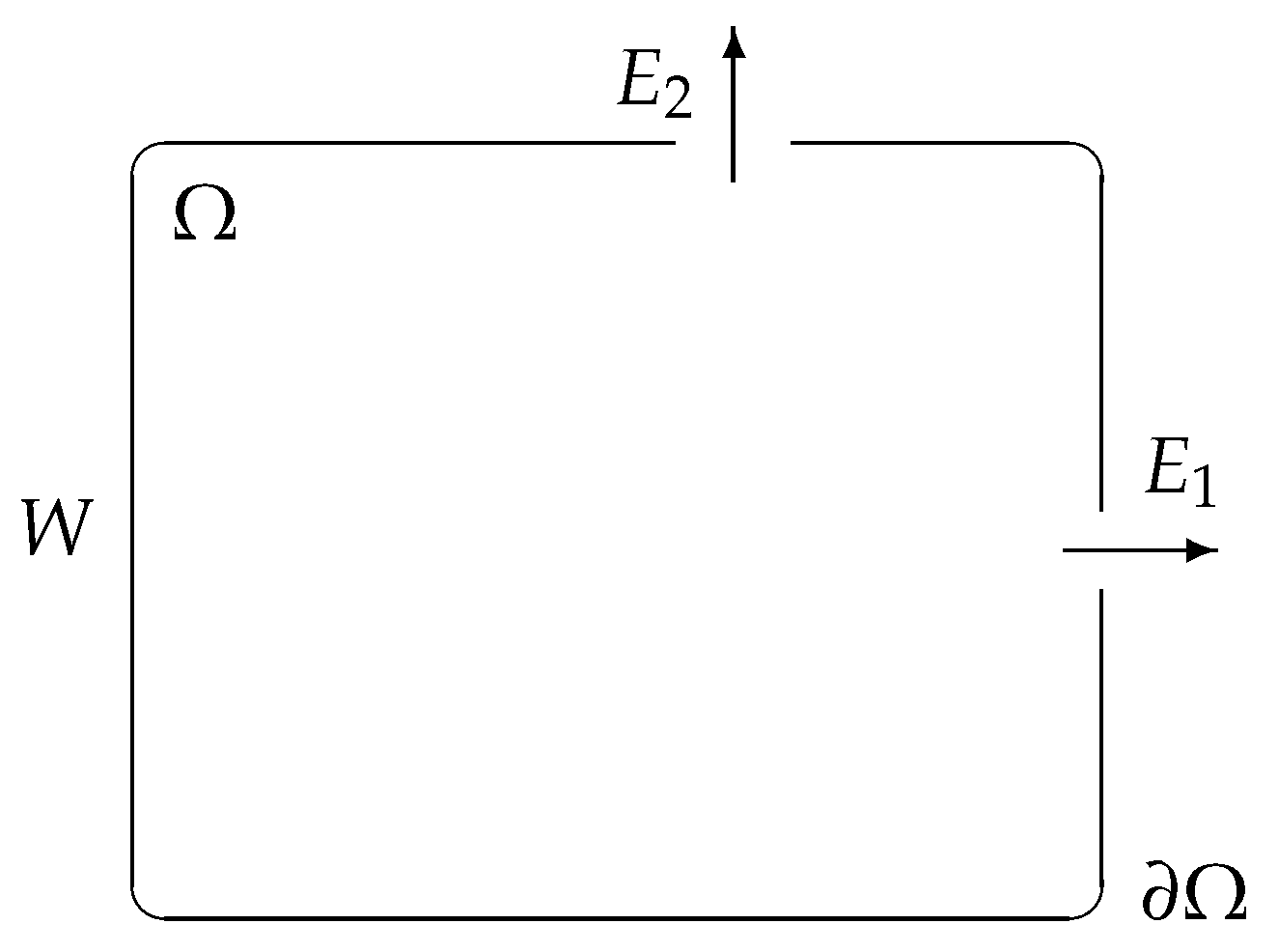
Figure 2.
Schematic representation of the features that are considered in the model and the microscopic variables over they have influence.
Figure 2.
Schematic representation of the features that are considered in the model and the microscopic variables over they have influence.

Figure 3.
(a) We denote the distance to the exit of a particle located in by and the vector pointing from to the exit by . (b) A particle in moving with direction is expected to collide the wall in , then it computes the tangent direction to the wall that would take it toward the exit.
Figure 3.
(a) We denote the distance to the exit of a particle located in by and the vector pointing from to the exit by . (b) A particle in moving with direction is expected to collide the wall in , then it computes the tangent direction to the wall that would take it toward the exit.

Figure 4.
Evolution of the total number of exposed pedestrians over time. Each scenario indicates its evacuation time. Once completed, the number of exposed individuals remains constant until the evacuation of all scenarios is finished.
Figure 4.
Evolution of the total number of exposed pedestrians over time. Each scenario indicates its evacuation time. Once completed, the number of exposed individuals remains constant until the evacuation of all scenarios is finished.
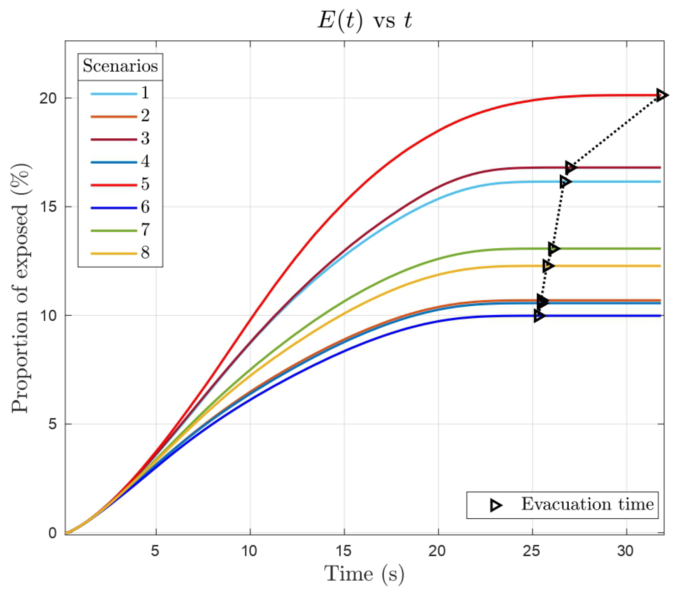
Figure 5.
Evolution of the evacuation process for scenarios 5 and 6 from Case Study 1. In scenario 5 (top row) pedestrians focus on finding the exit and tend to crowd together. In scenario 6 (bottom row) pedestrians tend to look for less crowded paths.
Figure 5.
Evolution of the evacuation process for scenarios 5 and 6 from Case Study 1. In scenario 5 (top row) pedestrians focus on finding the exit and tend to crowd together. In scenario 6 (bottom row) pedestrians tend to look for less crowded paths.
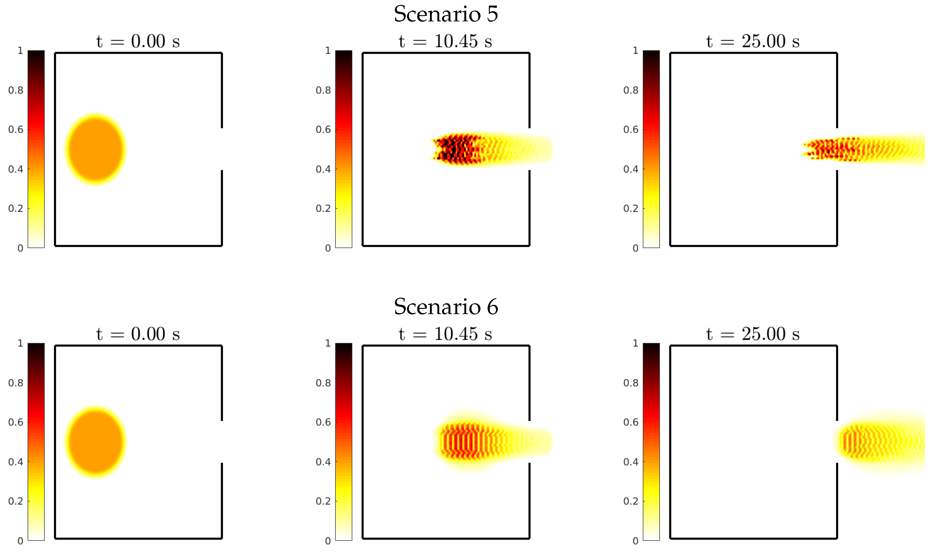
Figure 6.
Evolution of the total number of pedestrians with a given level of awareness over time. In each figure, the nodes represent the total number of pedestrians with awareness level , for , at time t, given by (9). To show the evolution with respect to time t, the proportions of pedestrians at each level are connected by segments. The arrows indicate where the changes in the levels of awareness occur.
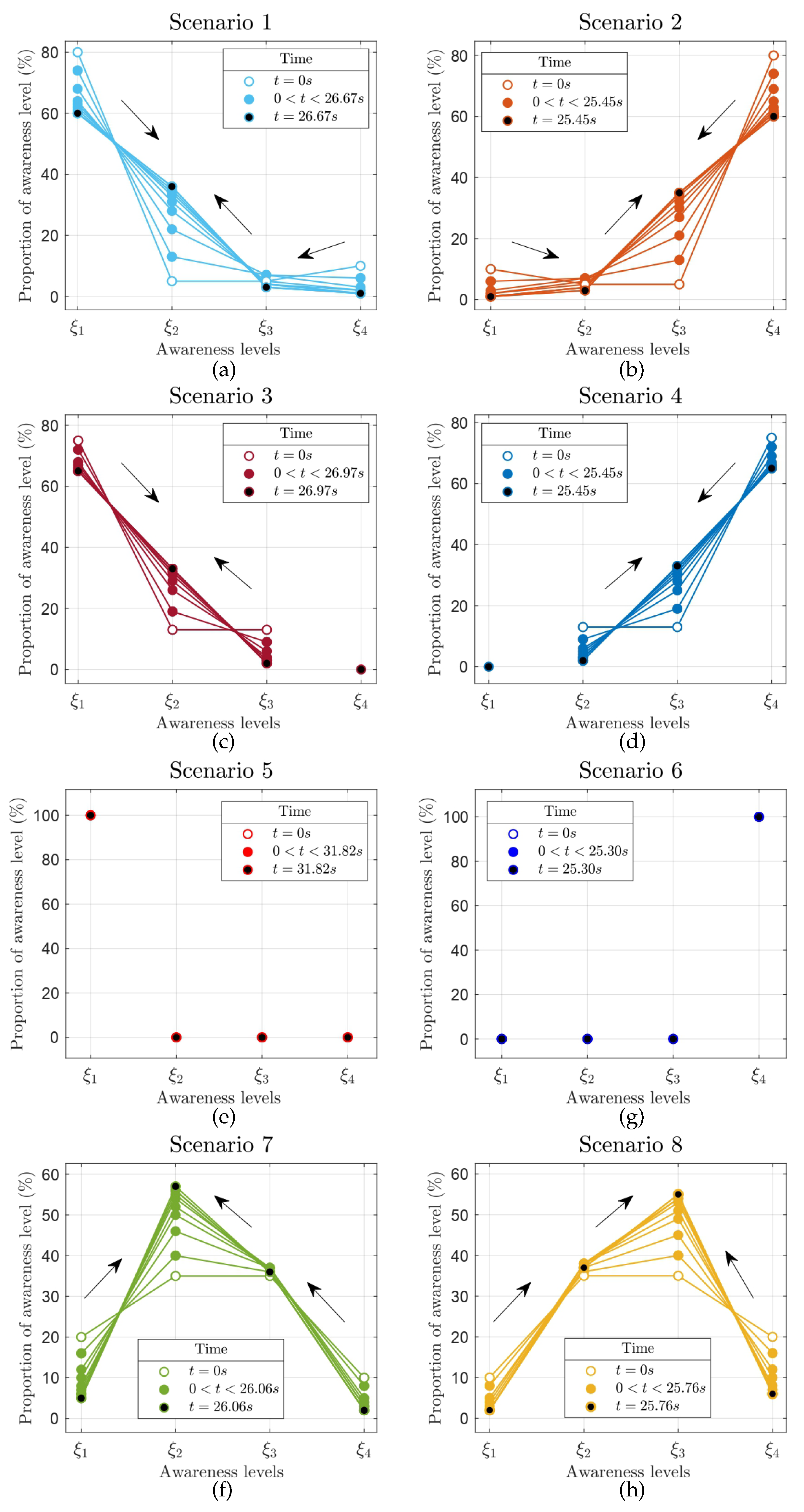
Figure 7.
Evolution of the minimum velocity reached by pedestrians over time for the different scenarios of Case Study 1.
Figure 7.
Evolution of the minimum velocity reached by pedestrians over time for the different scenarios of Case Study 1.
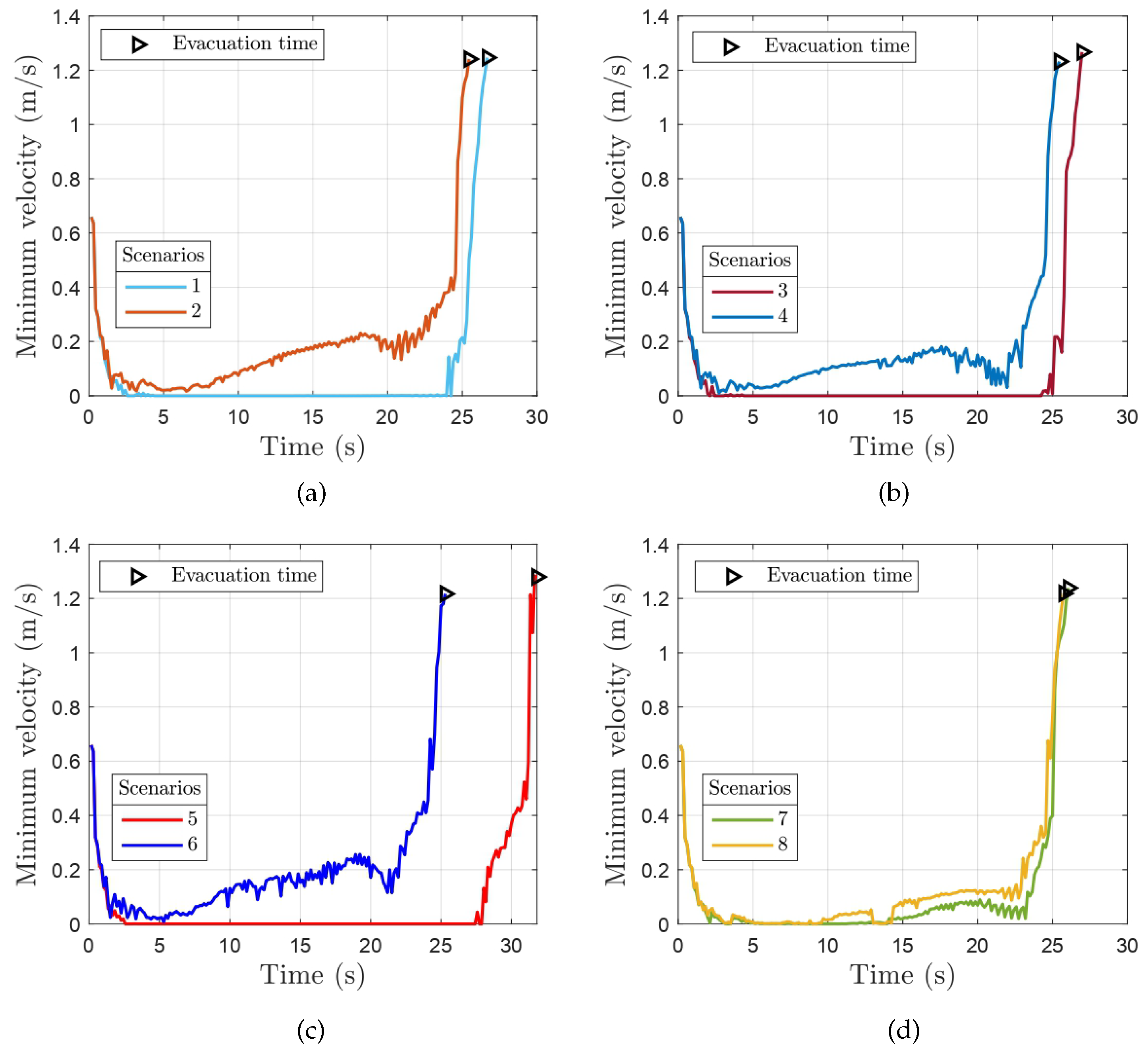
Figure 8.
Results of the Case Study 2. (a) Evolution of the total number of exposed pedestrians over time for each scenario. (b) Evolution of the total number of susceptible and vaccinated with respect to time for each scenario.
Figure 8.
Results of the Case Study 2. (a) Evolution of the total number of exposed pedestrians over time for each scenario. (b) Evolution of the total number of susceptible and vaccinated with respect to time for each scenario.
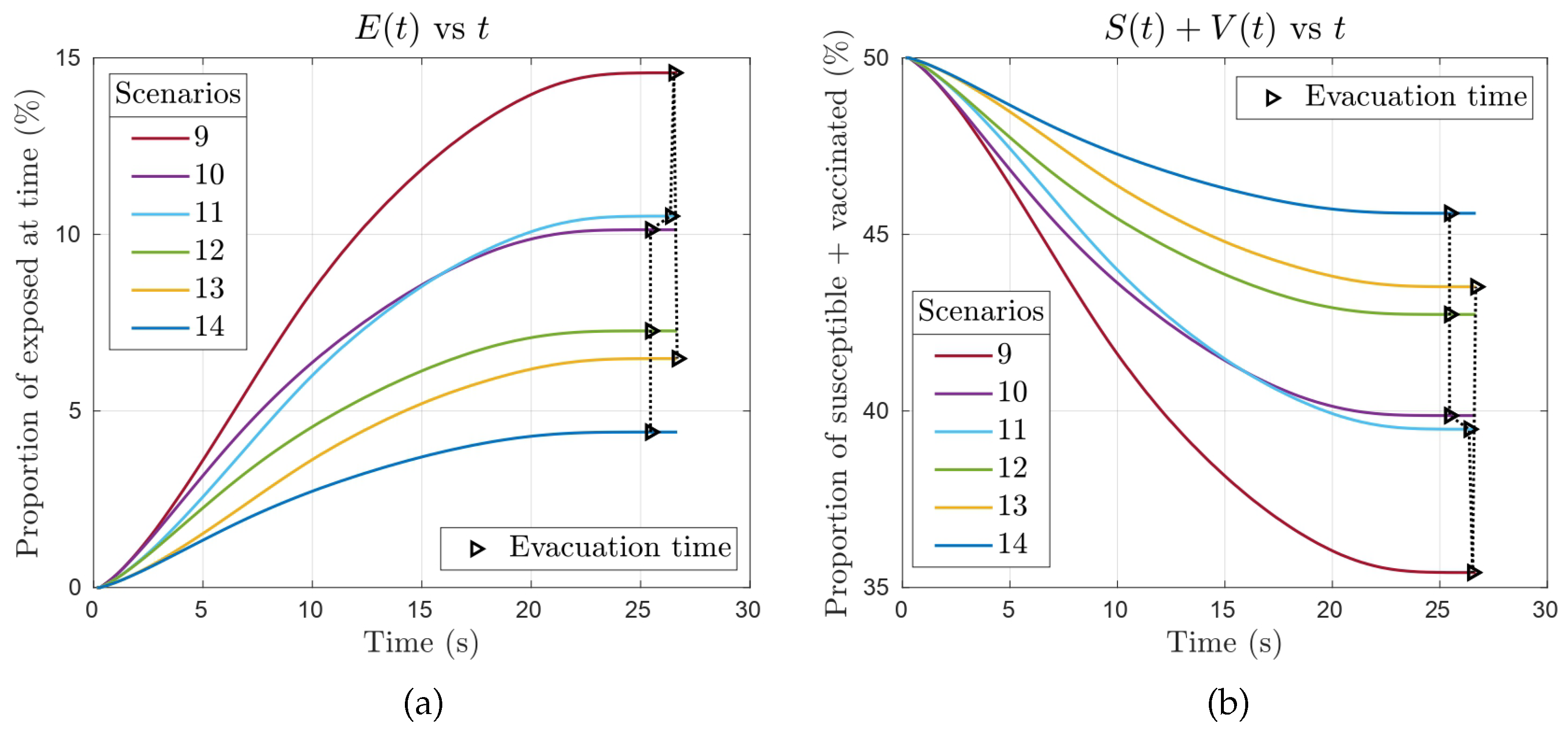
Figure 9.
Evolution of the evacuation process for scenarios 10 and 11 from Case Study 2. In scenario 10 (top row) pedestrians tend to look for less crowded paths. In scenario 11 (bottom row) pedestrians focus on finding the exit and tend to crowd together causing an increase in contagion of a infectious disease.
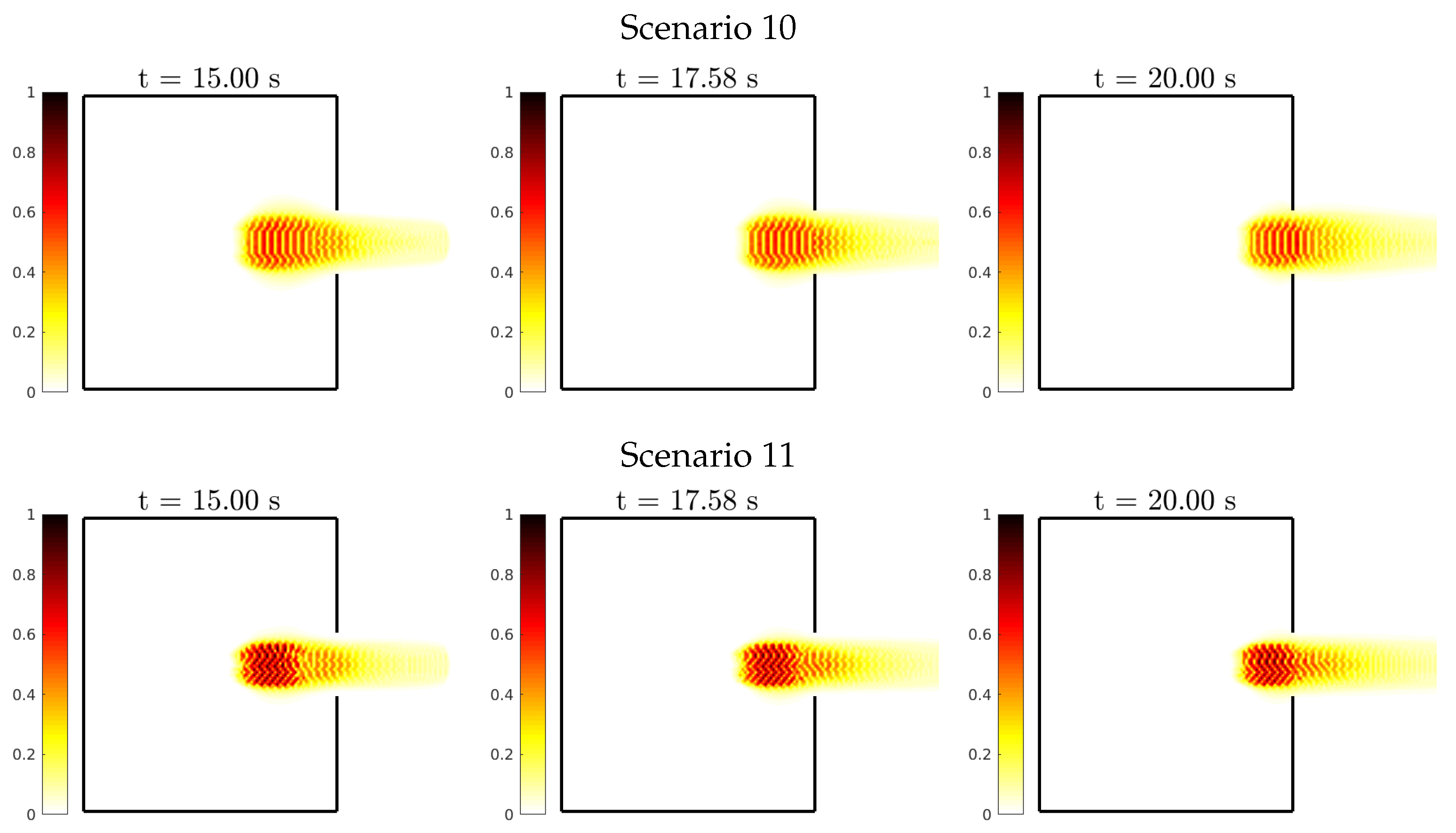
Figure 10.
Results of Case Study 3. (a) Evolution of the total number of exposed pedestrians over time for each scenario. (b) The three different functions considered. The values of the linear, quadratic and cubic functions at awareness levels , , are represented by a triangles, squares and diamonds, respectively.
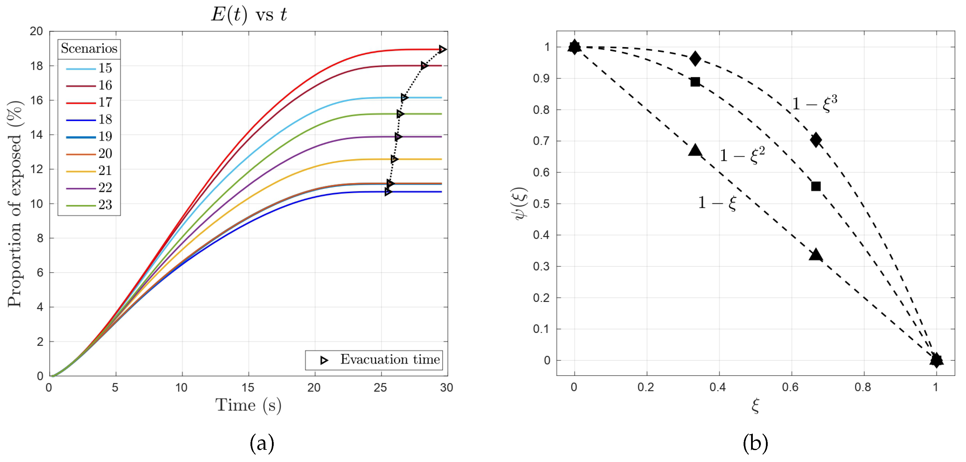

Table 1.
Scenarios considered in Case Study 1. Initial proportions for awareness and infectious levels are shown, as well as the definition of function .
Table 1.
Scenarios considered in Case Study 1. Initial proportions for awareness and infectious levels are shown, as well as the definition of function .
| Scenarios | Initial proportion of individuals (%) and function | ||||||||
|---|---|---|---|---|---|---|---|---|---|
| 1 | 80 | 5 | 5 | 10 | 75 | 25 | 0 | 0 | |
| 2 | 10 | 5 | 5 | 80 | 75 | 25 | 0 | 0 | |
| 3 | 75 | 0 | 75 | 25 | 0 | 0 | |||
| 4 | 0 | 75 | 75 | 25 | 0 | 0 | |||
| 5 | 100 | 0 | 0 | 0 | 75 | 25 | 0 | 0 | |
| 6 | 0 | 0 | 0 | 100 | 75 | 25 | 0 | 0 | |
| 7 | 20 | 35 | 35 | 10 | 75 | 25 | 0 | 0 | |
| 8 | 10 | 35 | 35 | 20 | 75 | 25 | 0 | 0 | |
Table 2.
Scenarios considered in case study 2. Initial proportions for infectious levels and awareness levels are shown, as well as the definition of function .
Table 2.
Scenarios considered in case study 2. Initial proportions for infectious levels and awareness levels are shown, as well as the definition of function .
| Scenarios | Initial proportion of individuals (%) and function | ||||||||
|---|---|---|---|---|---|---|---|---|---|
| 9 | 50 | 0 | 80 | 5 | 5 | 10 | |||
| 10 | 50 | 0 | 10 | 5 | 5 | 80 | |||
| 11 | 25 | 50 | 0 | 25 | 80 | 5 | 5 | 10 | |
| 12 | 25 | 50 | 0 | 25 | 10 | 5 | 5 | 80 | |
| 13 | 50 | 0 | 80 | 5 | 5 | 10 | |||
| 14 | 50 | 0 | 10 | 5 | 5 | 80 | |||
Table 3.
Scenarios considered in case study 3. Initial proportions for awareness levels and infectious levels as well as the definition of the different functions to be considered.
Table 3.
Scenarios considered in case study 3. Initial proportions for awareness levels and infectious levels as well as the definition of the different functions to be considered.
| Scenarios | Initial proportion of individuals (%) and function | ||||||||||
|---|---|---|---|---|---|---|---|---|---|---|---|
| 15 | 80 | 5 | 5 | 10 | 75 | 25 | 0 | 0 | |||
| 16 | 80 | 5 | 5 | 10 | 75 | 25 | 0 | 0 | |||
| 17 | 80 | 5 | 5 | 10 | 75 | 25 | 0 | 0 | |||
| 18 | 10 | 5 | 5 | 80 | 75 | 25 | 0 | 0 | |||
| 19 | 10 | 5 | 5 | 80 | 75 | 25 | 0 | 0 | |||
| 20 | 10 | 5 | 5 | 80 | 75 | 25 | 0 | 0 | |||
| 21 | 25 | 25 | 25 | 25 | 75 | 25 | 0 | 0 | |||
| 22 | 25 | 25 | 25 | 25 | 75 | 25 | 0 | 0 | |||
| 23 | 25 | 25 | 25 | 25 | 75 | 25 | 0 | 0 | |||
Disclaimer/Publisher’s Note: The statements, opinions and data contained in all publications are solely those of the individual author(s) and contributor(s) and not of MDPI and/or the editor(s). MDPI and/or the editor(s) disclaim responsibility for any injury to people or property resulting from any ideas, methods, instructions or products referred to in the content. |
© 2024 by the authors. Licensee MDPI, Basel, Switzerland. This article is an open access article distributed under the terms and conditions of the Creative Commons Attribution (CC BY) license (http://creativecommons.org/licenses/by/4.0/).
Copyright: This open access article is published under a Creative Commons CC BY 4.0 license, which permit the free download, distribution, and reuse, provided that the author and preprint are cited in any reuse.


