
Submitted:
25 November 2024
Posted:
26 November 2024
You are already at the latest version
Abstract
The inventory of carbon stocks in forests and the assessment of their spatio-temporal variability is a crucial task in the context of climate change and the search for adaptation strategies, as noted at both international and national levels. Since 2022, Russia has been implementing the project “Rhythm of Carbon”, one of the main goals of which is the assessment of carbon stocks in forests on permanent sites, which should be further upscaled using remote methods. We conducted the assessment of carbon stocks in tree stem biomass in a mixed boreal forest at the “Mukhrino” field station (West Siberia) using a comprehensive approach based on UAV LiDAR surveys and ground verification. Allometric models based on an ensemble approach and stochastic modeling were used to assess the relationship between ground-determined wood biomass stocks and tree height obtained via LiDAR. We obtained sufficient agreement between ground-based and remote assessments of tree heights, their number, and carbon stocks, which averaged 54 ± 11 t/ha. However, the LiDAR assessment conducted from a flight altitude of 120 meters does not account for understory trees due to the high canopy closure and systematically underestimates the number of overstory trees, which was compensated for using a correction factor.
Keywords:
forest inventory
; allometric models
; stochastic modeling
1. Introduction
Forests are the most important terrestrial ecosystems, providing accumulation and long-term storage of biogenic carbon in the form of timber and soil horizons rich in organic matter [1,2]. Inventorying forests' carbon stocks and assessing their spatiotemporal variability is a critical task in the context of climate change and the search for ways to adapt to it, as noted at both international [3] and national [4] levels. Since 2022, Russia has been implementing the project "National system for monitoring carbon pools and greenhouse gas fluxes in Russia" ("Rhythm of Carbon"), one of the main goals of which is the assessment of carbon stocks in forest ecosystems, which is already being carried out at the developing network of permanent monitoring stations [5].
The most significant carbon pool of boreal forests is the phytomass of stem wood, which accumulates up to 20–30% of carbon in such ecosystems [1,6]. Traditionally, the inventory of stem wood stocks (and consequently carbon) in forests is carried out using field forest inventory methods on standard sample plots of 50×50 to 100×100 meters. Such data requires further scaling in space and time to inventory of carbon stocks at local and regional levels [7,8,9].
Upscaling information obtained on the ground is conveniently done using remote sensing satellite data: information on location, condition, and predominant tree species is available in the visible and multispectral ranges [7,10,11,12,13,14]; in the lidar and radar ranges, information on tree height and crown sizes is available [15,16,17,18,19]. However, the resolution of open satellite data (Landsat, Sentinel) is often insufficient for accurate interpretation of ground information both spatially and temporally, especially at the level of individual forest inventory plots of small size, and commercial imagery is expensive and does not always sufficiently cover the territory for which upscaling is carried out [20,21].
The link between ground and satellite data in the process of their spatial and temporal interpretation can be effectively achieved using unmanned aerial vehicles (UAVs). They allow for the identification of small-scale (at the level of individual trees) areas of forest cover degradation and recovery, obtaining information on forest productivity, predominant tree species, phenological stage, fires, and pest spread. In addition, LiDAR sensors installed on UAVs enable the assessment of the vertical structure of forest communities, morphological characteristics of the stand, features of the underlying terrain, stratification, tree growth dynamics, and the condition of individual trees. It should be emphasized that data at the level of individual trees (sub-centimeter resolution) can only be obtained using UAVs, which significantly expands the capabilities of ground-based forest inventory work for upscaling, including with the help of satellite data [22,23,24].
Tree height, assessed using LiDAR UAVs, is a key parameter in evaluating woody biomass stocks; when combined with considerations of tree species, crown projective cover, and trunk diameter, it is sufficiently accurate for calculating carbon stocks in them [25,26], especially in the presence of allometric models with carefully identified parameters. Determination of tree heights is performed using a three-dimensional point cloud of laser reflections (LiDAR), obtained by recording the direction and travel time of the laser scanner beam from source to receiver, with a root mean square error of about 1–10 cm [27,28], which is comparable to or more accurate than ground-based assessment.
Remote LiDAR data require careful processing and ground verification: errors in estimating the number and height of trees often arise under conditions of rugged terrain, high canopy closure, low tree heights, and insufficient density of the point cloud of laser reflections or small overlap area of images for photogrammetric processing. In [29], it was noted that measuring tree height based on LiDAR surveying tends to underestimate the height of tall trees and overestimate the height of short trees; in [30], it was shown that some algorithms for processing LiDAR data tend to underestimate or overestimate tree heights; according to our earlier studies [31], when assessing the height of tree cover in an oligotrophic bog area (low-growing pines with an average height of up to 3 meters) using LiDAR surveying, a systematic underestimation of tree height was noted. Nevertheless, approaches based on the use of LiDAR surveying contribute to obtaining sufficiently accurate and reproducible results in the assessment of morphological properties of tree cover [27,28,30].
This work is dedicated to the verification of stem wood carbon stocks obtained from LiDAR UAV surveying by means of ground-based forest inventory in a mixed boreal forest site in Western Siberia.
2. Materials and Methods
2.1. Study Area
The research was conducted at the mixed forest site of the international field station "Mukhrino," located on the left bank of the Ob and Irtysh rivers, 20 km southwest of the city of Khanty-Mansiysk, Russia [32], in June 2023 (Figure 1). The mixed forest site, measuring 1.5×4.5 km (center coordinates: N60.897437 E68.711363), is a permanent plot for ground-based carbon stock assessment, which will be scaled up (together with other plots as part of the development of the observation network) to the territory of Russia within the "Rhythm of Carbon" project using satellite remote sensing data and mathematical modeling. The study area is located in the middle taiga of the boreal biogeographical zone, and the mixed herbaceous-green-moss forest with a canopy closure of 70-80% consists of two layers. In the first tree layer, aspen (Populus tremula), birch (Betula pubescens), siberian pine (Pinus sibirica), fir (Abies sibirica), and spruce (Picea obovata) predominate. The understory layer includes fir, siberian pine, and spruce. The undergrowth mainly comprises siberian pine, fir, spruce, and aspen. The total number of live undergrowth ranges from 7000 to 19000 plants per hectare. The stand is of III–IV site class, reaching heights of 20–25 m and trunk diameters of 30–50 cm. The understory is poor in species composition, mainly represented by rowan, and more rarely by rosehip. The number of understory plants ranges from 400 to 3800 per hectare. In the ground cover, taiga small grassy plants dominate – Linnaea borealis, Maianthemum bifolium, Gymnocarpium dryopteris, and boreal species of green mosses Hylocomium splendens and Pleurozium schreberi. Less abundantly, there is Vaccinium myrtillus, Equisetum sylvaticum and species of clubmosses like Diphaziastrum complanatum and Lycopodium annotinum. The forest represents a climax stage of development on well-drained sandy loam and loamy podzols. These mixed forests are typical for the middle taiga of Western Siberia and are often associated in the landscape with excessively moist types, such as swampy birch-sedge (Carex globularis) sphagnum (Sphagnum angustifolium) and horsetail-small grassy forests, as well as at the borders with bogs, the so-called "ryams", which often form continuous landscape gradients. Ryam is a type of forested bog characterized by a shrub layer of Ledum palustris and Chamaedaphne calyculata, with the participation of Vaccinium myrtillus, and a tree layer of 6–10 meters high Pinus sylvestris with a small admixture of Siberian cedar (P. sibirica), birch (Betula pubescens), and predominance in the ground cover of Sphagnum angustifolium and Sphagnum divinum.
2.1. Forest Taxation And Allometric Models
In the mixed forest, 5 sample sites were established (the coordinates of the site centers are presented in Table 1) for conducting forest inventory, which included: a complete enumeration of trees with separation by layers and represented species, measurement of tree heights (using a SUUNTO PM-5/1520 hypsometer) and diameters at breast height (at 1.3 m using a diameter caliper), assessment of above-ground phytomass, as well as evaluation of wood density in model trees considering layers and species.
The aboveground phytomass of the model trees (one average tree for height and diameter in each of the two layers of each sample plot) was determined for the overstory layer by direct weighing of the sawn trunk using KERN CH50K scales; and for the trees of the understory layer – by calculation (by allometric model).
To achieve this, the trunk volume was calculated (equation 1) and the wood density was measured (equation 2) in disks with a thickness of 3–4 cm, cut out from the middle of two-meter trunk sections (at odd meters).

where: Vg – trunk volume, m3; l – section length, m (all sections except the top had a length of 2 m); si – cross-sectional area in the middle of the two-meter section (at odd meters, the index i corresponds to the height in meters, for example, s1 – area at a height of 1 m, s3 – at a height of 3 m, etc.), m2 (measured for the cut disks); stop – cross-sectional area at the base of the tree top, m2; ltop – length of the tree top, m.
where: ρ – density of the cut disk, kg/m3; m – mass of the disk, kg; Vd – volume of the disk, m³. The mass of the disk was determined using KERN 440-47 scales. The volume of the disk was determined by four measured diameters (in different directions, averaged) and by eight measurements of thickness (also averaged). The mass of each two-meter section was obtained by multiplying the density of the corresponding disk ρ by the volume of the corresponding two-meter section; the sum of the masses of all sections was equal to the trunk phytomass.
The weighted average wood density for each of the five studied plots was calculated using equation 3.
где: ρw – is the average weighted density of wood in the area, kg/m3; ρi – is the density of the wood of the i-th species of trees in the area, kg/m3; wi – is the dimensionless weight coefficient calculated as the ratio of the mass of the trunks of the i-th species of trees to the total mass of the trunks of all trees in the area; n – is the number of species of trees in the area.
The biomass stocks of tree trunks on each of the five sample plots were determined according to formula 4:

where: AGBg, j – biomass stock of stem-wood calculated based on ground-data for the j-th sample plot, kg; nj – number of trees on the j-th sample plot; ρm – average (across all plots) wood density, kg/m3; Vk,j – volume of the k-th tree on the j-th sample plot, m3.
The dependence of tree trunk diameters on height was determined using the multi-model technique. For this, the parameters of three simple regression allometric models were identified based on field data obtained from all five plots, and the median value of the results was calculated (equation 5).
where: dmod – modeled trunk diameter (at a height of 1.3 m), m; h – tree height, m; model parameters: a, m; b, 1/m; c, m (this parameter includes the normalization factor h0, m); e и d – dimensionless model parameters. The error in parameter identification was calculated using stochastic modeling [33,34]: random numbers with a uniform distribution in the range of five times the ground measurement error were added to the input data, which for trunk diameter ranged from ─0.05 to 0.05 m, and for tree height – from ─0.5 to 0.5 m); based on the resulting data, parameter identification of the model was performed by least-squares fitting (minimizing the sum of the squares of the differences between the measured and modeled diameter). This procedure was repeated 1000 times, resulting in 1000 sets of model parameters. For each parameter, the mean and standard deviation were calculated from its 1000 realizations. Models with identified parameters were then used to calculate the trunk volume based on their height obtained using lidar surveying, as described below.
2.2. LiDAR Data Acquisition and Processing
Lidar surveying was conducted in July 2023 in a mixed forest at the "Mukhrino" study site, covering an area of 662 hectares, using a UAV DJI Matrice 300 and a DJI Zenmuse L1 lidar. The UAV flight altitude was 120 meters above the surface, with the lidar oriented vertically downwards (nadir), and the scanning angle varied between ─35° and 35°. The point cloud density of laser reflections (LiDAR) was 102 points/m2, ground sampling distance – 3.27 cm/pixel, flight speed – 12 m/s, transverse overlapping of LiDAR – 50%. Initial processing of the point cloud of laser reflections (LiDAR) included the alignment and smoothing of LiDAR to eliminate artifacts caused by distance measurement errors, noise, and UAV movements using DJI Terra, and then the data were exported in .las format.
Segmentation of individual tree crowns and calculation of their height based on LiDAR was performed using the "Lidar toolbox" module in MATLAB 2023a. The module requires the specification of two main parameters: "gridRes" – the size of the moving window for creating the canopy height model and "minTreeHeight" – the minimum tree height considered. In practice, for low-density LiDAR (about hundreds of points per m2), obtained for a forest with high crown closure and little variability in tree heights, the "Lidar toolbox" tends to underestimate the number of trees due to the "merging" of several plants into one during segmentation [19,31]. However, the degree of "underestimation" decreases as the "gridRes" parameter value decreases. Therefore, to analyze tree heights across the entire study site with the given LiDAR density, we selected the minimum functional value of the "gridRes" parameter = 0.3 m, and set the "minTreeHeight" to 5 m.
The result of the LiDAR segmentation was exported from MATLAB 2023a as two vector files in .shp format: a point file representing the tree crown vertex locations (with coordinates in the WGS84 42N projection in the attribute table) and a polygon file corresponding to the boundaries of segmented tree crowns.
2.3. Calculation of Carbon Storage And Their Ground Verification
As described above, the assessment of carbon stock in trunk wood was based on field data on the ratio of tree heights and trunk diameters (calculated using an ensemble of simple allometric models), the number of trees in the studied plots, and the wood density in them. The trunk diameters (dmod) were calculated at the study site based on the height data obtained using lidar surveying (hLIDAR), and from this, the cross-sectional area was calculated using equation 6:
where: smod – cross-sectional area of trees (at a height of 1.3 m), m2; dmod – modeled trunk diameter (at a height of 1.3 m), m.
Based on the known height and cross-sectional area of trees, the merchantable volume (assuming the trunk has the shape of a cone) was calculated using equation 7:
where: Vm – merchantable volume, m3; hLIDAR – tree height obtained from lidar surveying, m; smod – cross-sectional area of trees (at a height of 1.3 m), m2; dmod – modeled trunk diameter (at a height of 1.3 m), m; d1/2 – diameter of the trunk at half the tree height (m), which was calculated using equation 8:

where: d1/2 – diameter of the trunk (at half the tree height, m); hLIDAR – tree height obtained from lidar surveying, m. The biomass stocks of tree trunks on each of the five sample plots were determined using equation 9:

where: AGBLIDAR, j – biomass stocks of stem wood calculated based on LIDAR data for the j-th sample plot, kg; Vm,k,j – merchantable volume calculated using equation 7 for the k-th tree on the j-th sample plot, m3. The obtained merchantable volume of trunk wood (Vm) was converted to carbon stock using equation 10:
where: С – carbon stock in tree trunks, kg; α – dimensionless ground verification coefficient, identified by minimizing the sum of squares of the differences between the aboveground biomass stocks determined for each of the five sample plots both on the ground (AGBg,i) and remotely (AGBLIDAR,i); AGBLIDAR – biomass stocks of tree trunks for the entire study site; Cfrac – average weighted carbon fraction in tree trunks, calculated taking into account the number of coniferous and deciduous trees on the plots (similarly to ρw, according to the data [35] and [36]), and equal to 0.5.
3. Results
3.1. Forest Taxation and Allometric Models
In the result of ground forest inventory on sample plots 1–5, there were found 90, 66, 83, 92, and 59 trees in the overstory layer and 277, 196, 190, 202, and 212 in the understory layer respectively. The median (1Q, 3Q) height of trees in the overstory layer was 27 (24, 29), 26 (17, 28), 29 (23, 31), 27 (25, 29), and 29 (27, 30) m, and in the understory layer it was 15 (14, 17), 14 (13, 15), 14 (11, 17), 15 (13, 18), and 15 (13, 18) m. The median (1Q, 3Q) diameters of tree trunks in the overstory layer at a height of 1.3 m were 29 (24, 34), 25 (16, 33), 34 (24, 42), 29 (24, 36), and 41 (29, 49) cm, and in the understory layer they were 13 (11, 14), 12 (11, 13), 14 (10, 16), 13 (12, 16), and 13 (12, 16) cm. The average weighted wood density ρw varied slightly across the sample plots and was on average 0.43±0.02 t/m3. The biomass stocks AGBg,i were 152, 107, 156, 148, and 137 t/ha respectively.
3.2. Characteristics of the Forest stand Based on LiDAR data
In the result of assessing the stand characteristics based on LiDAR data, 41, 30, 37, 44, and 27 trees were found on sample plots 1–5 respectively. The number of trees identified using the LiDAR survey was significantly underestimated compared to the results of ground forest inventory (Figure 3): both for the number of overstory trees and for overstory and understory trees combined. Nevertheless, an extremely strong linear regression relationship (R2 = 0.98) was found between the number of overstory trees determined on the ground and based on the LiDAR survey, while the relationship between the total number of trees determined on the ground and remotely was relatively low (R2 = 0.36).
The median (1Q, 3Q) height of trees (without layer separation) obtained based on LiDAR data was 28 (26, 29), 27 (25, 29), 30 (29, 31), 28 (25, 29), and 28 (26, 30) m. The Mann-Whitney U-test, conducted to compare the heights obtained from LiDAR data and ground assessment (with separation into all trees and overstory trees) showed no significant differences only between LiDAR and overstory trees on plots 4 and 5 (p = 0.29 and 0.75 respectively, Figure 4). It is evident that LiDAR data with the survey parameters specified in section 2.2 are insufficient for inventorying trees below 22–24 m in height, which does not allow for height assessment beyond the overstory layer. In most cases (sites 1–4), the median height of trees obtained from LiDAR data is 1–2 m higher than that obtained using ground data for the overstory layer.
The modeled median (1Q, 3Q) diameter of tree trunks (without layer separation) at a height of 1.3 m was 33 (29, 39), 32 (26, 38), 39 (34, 44), 33 (27, 38), and 34 (29, 41) cm (Figure 5). The uncertainty (1Q, 3Q) in the results of modeling the median tree diameter on the plots includes two types of errors caused by: 1) natural variability in tree diameters on each plot and 2) error in model parameter identification; 1Q was calculated for the results of dmod obtained from an ensemble of models using parameters identified at the lower uncertainty bound, and 3Q was calculated at the upper uncertainty bound (Table 2). As with the assessment of tree heights, the medians of the modeled diameters based on LiDAR data significantly differed from the ground assessment (except for site 3, p = 0.28). In most cases (sites 1–4), the median diameter of trees obtained from LiDAR data was 4–7 cm larger than those obtained using ground data for the overstory layer.
The modeled total biomass stocks for plots 1–5 (AGBLIDAR,i) thus included the combined uncertainty of modeling the median diameter and assessing the tree height, and amounted to 65 (55, 75), 44 (38, 50), 80 (65, 95), 71 (59, 83), and 46 (38, 54) t/ha respectively. Nevertheless, they closely correlated with AGBg,i obtained from ground data (Figure 6).
3.3. Ground verification of AGB and Calculation of Carbon Storage
The underestimation of biomass stocks obtained from LiDAR data was corrected by introducing a correction factor α = 2.2 (equation 10), used to minimize the RMSE. The results of the biomass stock adjustment are presented in Figure 7: RMSE was reduced from 80 to 32, approaching a 1:1 ratio between ground and remote assessments.
The obtained estimate αAGBLIDAR was used to calculate the carbon stocks for the entire study area (S = 662 ha), which amounted to 35814±6915 tC or 54±11 t/ha. The spatial variability of carbon stocks in the study area is presented in Figure 8: it ranged from 5±1 tC/ha in areas bordering wetlands to 110±21 tC/ha in forest areas occupied by cedar and mature mixed stands.
4. Discussion
The calculated biomass stocks before the introduction of the correction factor α differed by 2.2 times from those obtained through ground assessment. We assume that the main contribution to this underestimation came from the unrecorded overstory and understory trees during the LiDAR survey: the number of identified overstory layer was underestimated by 2.2 times, and the understory layer of trees were completely ignored (as confirmed by the median tree height assessment on the trial plots – Figure 4). The reason for ignoring the understory trees is the high canopy closure of the overstory layer, which were themselves undercounted due to the low density of the point cloud during the LiDAR survey. To obtain a higher point cloud density, it is necessary to increase lateral overlap during the LiDAR survey, reduce the flight altitude, or conduct multiple surveys of the same area. Accounting for lower layer trees could be done in the fall period with fallen leaves, which could increase the number of reflected LiDAR signals from beneath the forest canopy. Nevertheless, the high correlation of tree counts obtained by ground (for the overstory layer) and remote assessment indicates a systematic error that can be effectively compensated, as shown above.
The systematic overestimation of the median tree height is insignificant (1–2 m, except for plot 5) and can also be explained by the unaccounted trees below 22–24 meters, which might have shifted the median assessment. The overestimation of tree diameters calculated (by 4–7 cm, again except for plot 5), may be due to the assumption that trees take the shape of a cone. It is noteworthy that the absence of diameter and height overestimation is characteristic only for plot 5, where the least number of trees were found among all the plots, suggesting that the process of obtaining reliable LiDAR surveys and tree identification is more accurate for sparse stands.
We compared the carbon stocks of the forest we studied with estimates available in the literature (Table 3). In the table, we showed the results of the current study for forest plots on relatively drained sites, and it largely coincides with the literature data for similar forests. The average carbon stock of stem wood across the entire study area is close to the lower limit of estimates for similar forests, due to the presence of a large number of bog areas (about 9% of the territory) as well as a river crossing the forest and its floodplain (7%). Of the 662 hectares, the forest areas directly occupy about 556 hectares, many of which are represented by low-productivity communities: if the total carbon stock is recalculated for the actual area they occupy, the specific carbon stock will be 64 t/ha. At the same time, the average value obtained from all analyzed works is 83 t/ha. It should be noted that in the latter case some authors included not only stem wood but also the biomass of branches and photosynthesizing organs of trees, which was not the aim of our study.
Testing the technology for accounting the total aboveground biomass of trees, as well as accounting for the spatial variability of their species composition, will be the topic of our further work.
Author Contributions
Conceptualization, D.V.I.; methodology, D.V.I. and A.A.K.; software, A.A.E. and A.V.K; validation, D.V.I and M.V.G.; formal analysis, D.V.I, A.A.E and M.V.G.; investigation, A.A.K; resources, A.A.K., I.V.K and M.F.K; data curation, D.V.I, I.V.K and A.A.E.; writing—original draft preparation, D.V.I, M.V.G. and V.A.R.; writing—review and editing, M.V.G.; visualization, D.V.I and A.A.E; supervision, D.V.I; project administration, D.V.I; funding acquisition, D.V.I. All authors have read and agreed to the published version of the manuscript.
Funding
The remote (LiDAR) assessment of tree biomass was funded by the state assignment of Ministry of Science and Higher Education of the Russian Federation to organize a new young researcher Laboratory in Yugra State University (Research number 1022031100003-5-1.5.1) as a part of the implementation of the National Project “Science and Universities”. Ground verification of tree biomass and APC was funded by the Government of the Tyumen region within the framework of the Program of the World-Class West Siberian Interregional Scientific and Educational Center (national project “Nauka”).
Data Availability Statement
Data is contained within the article
Acknowledgments
We are deeply grateful to Vladimir Bodash and all the engineers who provided logistical support at the Mukhrino field station. We would also like to express our special thanks to all the scientists, who conducted the ground verification of the data: Nagimov Z.Ya., Shevelina I.V., Usoltsev V.A., Bartsh A.A., Suslov A.V., Vorobyeva T.S., Orekhova O.N., Salnikova I.S., Anchugova G.V., Semyshchev S.G., Chudnov O., and Gromov A.M.
Conflicts of Interest
“The authors declare no conflicts of interest.”
References
- Dixon, R.K.; Solomon, A.M.; Brown, S.; Houghton, R.A.; Trexier, M.C.; Wisniewski, J. Carbon Pools and Flux of Global Forest Ecosystems. Science 1994, 263, 185–190. [Google Scholar] [CrossRef] [PubMed]
- Bradshaw, C.J.A.; Warkentin, I.G. Global Estimates of Boreal Forest Carbon Stocks and Flux. Global and Planetary Change 2015, 128, 24–30. [Google Scholar] [CrossRef]
- Lee, H.; Calvin, K.; Dasgupta, D.; Krinner, G.; Mukherji, A.; Thorne, P.; Trisos, C.; Romero, J.; Aldunce, P.; Barret, K.; et al. IPCC, 2023: Climate Change 2023: Synthesis Report, Summary for Policymakers. Contribution of Working Groups I, II and III to the Sixth Assessment Report of the Intergovernmental Panel on Climate Change [Core Writing Team, H. Lee and J. Romero (Eds.)]. IPCC, Geneva, Switzerland. Available online: https://doi.org/10.59327/IPCC/AR6-9789291691647.001 (accessed on 22 November 2024).
- Decree of the President of the Russian Federation dated November 4, 2020, No. 666 "On the reduction of greenhouse gas emissions." URL: http://www.kremlin.ru/acts/bank/45990 (access date: 13.08.2024).
- Kurganova, I.N.; Karelin, D.V.; Kotlyakov, V.M.; Prokushkin, A.S.; Zamolodchikov, D.G.; Ivanov, A.V.; Ilyasov, D.V.; Khoroshaev, D.A.; de Gerenyu, V.O.L.; Bobrik, A.A.; et al. A Pilot National Network for Monitoring Soil Respiration in Russia: First Results and Prospects of Development. Dokl. Earth Sc. 2024, 519, 1947–1954. [Google Scholar] [CrossRef]
- Ameray, A.; Bergeron, Y.; Valeria, O.; Montoro Girona, M.; Cavard, X. Forest Carbon Management: A Review of Silvicultural Practices and Management Strategies Across Boreal, Temperate and Tropical Forests. Curr Forestry Rep 2021, 7, 245–266. [Google Scholar] [CrossRef]
- Lister, A.J.; Andersen, H.; Frescino, T.; Gatziolis, D.; Healey, S.; Heath, L.S.; Liknes, G.C.; McRoberts, R.; Moisen, G.G.; Nelson, M.; et al. Use of Remote Sensing Data to Improve the Efficiency of National Forest Inventories: A Case Study from the United States National Forest Inventory. Forests 2020, 11, 1364. [Google Scholar] [CrossRef]
- Wang, D.; Wan, B.; Liu, J.; Su, Y.; Guo, Q.; Qiu, P.; Wu, X. Estimating Aboveground Biomass of the Mangrove Forests on Northeast Hainan Island in China Using an Upscaling Method from Field Plots, UAV-LiDAR Data and Sentinel-2 Imagery. International Journal of Applied Earth Observation and Geoinformation 2020, 85, 101986. [Google Scholar] [CrossRef]
- Order of The Russian Federal Forestry Agency (RFFA) dated May 6, 2022, No. 556 "On the approval of the Regulation on the organization and conduct of state forest inventory activities by the central apparatus of the RFFA, territorial bodies of RFFA, and organizations subordinate to RFFA." URL: https://rosleshoz.gov.ru/doc/пр№5562022.05.06 (access date: 14.01.2024).
- Reese, H.; Nilsson, M.; Sandström, P.; Olsson, H. Applications Using Estimates of Forest Parameters Derived from Satellite and Forest Inventory Data. Computers and Electronics in Agriculture 2002, 37, 37–55. [Google Scholar] [CrossRef]
- Hansen, M.C.; Potapov, P.V.; Moore, R.; Hancher, M.; Turubanova, S.A.; Tyukavina, A.; Thau, D.; Stehman, S.V.; Goetz, S.J.; Loveland, T.R.; et al. High-Resolution Global Maps of 21st-Century Forest Cover Change. Science 2013, 342, 850–853. [Google Scholar] [CrossRef] [PubMed]
- Bartalev, S.; Egorov, V.A.; Ershov, D.; Isaev, A.S.; Loupian, E.; Plotnikov, D.; Uvarov, I.A. Satellite Mapping of the Vegetation Cover over Russia Using MODIS Spectroradiometer Data. Contem Remote Sens Space 2011, 8, 285–302. [Google Scholar]
- Sochilova, E.N.; Surkov, N.V.; Ershov, D.V.; Khamedov, V.A. Assessment of Biomass of Forest Species Using Satellite Images of High Spatial Resolution (on the Example of the Forest of Khanty-Mansi Autonomous Okrug)9-9. Forest Science Issues 2019, 2, 9–9. [Google Scholar] [CrossRef]
- Puliti, S.; Breidenbach, J.; Schumacher, J.; Hauglin, M.; Klingenberg, T.F.; Astrup, R. Above-Ground Biomass Change Estimation Using National Forest Inventory Data with Sentinel-2 and Landsat. Remote Sensing of Environment 2021, 265, 112644. [Google Scholar] [CrossRef]
- Wallace, L.; Lucieer, A.; Watson, C.; Turner, D. Development of a UAV-LiDAR System with Application to Forest Inventory. Remote Sens. 2012, 4, 1519–1543. [Google Scholar] [CrossRef]
- Nilsson, M.; Nordkvist, K.; Jonzén, J.; Lindgren, N.; Axensten, P.; Wallerman, J.; Egberth, M.; Larsson, S.; Nilsson, L.; Eriksson, J.; et al. A Nationwide Forest Attribute Map of Sweden Predicted Using Airborne Laser Scanning Data and Field Data from the National Forest Inventory. Remote Sensing of Environment 2017, 194, 447–454. [Google Scholar] [CrossRef]
- Zhao, K.; Suarez, J.C.; Garcia, M.; Hu, T.; Wang, C.; Londo, A. Utility of Multitemporal Lidar for Forest and Carbon Monitoring: Tree Growth, Biomass Dynamics, and Carbon Flux. Remote Sensing of Environment 2018, 204, 883–897. [Google Scholar] [CrossRef]
- García, M.; Saatchi, S.; Ustin, S.; Balzter, H. Modelling Forest Canopy Height by Integrating Airborne LiDAR Samples with Satellite Radar and Multispectral Imagery. International Journal of Applied Earth Observation and Geoinformation 2018, 66, 159–173. [Google Scholar] [CrossRef]
- Cheng, J.; Zhang, X.; Zhang, J.; Zhang, Y.; Hu, Y.; Zhao, J.; Li, Y. Estimating the Aboveground Biomass of Robinia pseudoacacia Based on UAV LiDAR Data. Forests 2024, 15, 548. [Google Scholar] [CrossRef]
- Grün, A. Potential and limitations of high-resolution satellite imagery. In ACRS 2000: Proceedings of the 21st Asian Conference on Remote Sensing, Proceedings of the 21st Asian Conference on Remote Sensing, Taipei International Convention Center, Taipei, Taiwan, 4-8 December 2000; Center for Spaee & Remote Sensing Research, National Central University, Chinese Taipei Society of Photogrammetry and Remote Sensing, 2000.
- Zhao, Q.; Yu, L.; Du, Z.; Peng, D.; Hao, P.; Zhang, Y.; Gong, P. An Overview of the Applications of Earth Observation Satellite Data: Impacts and Future Trends. Remote Sens. 2022, 14, 1863. [Google Scholar] [CrossRef]
- Huang, C.; Homer, C.; Yang, L. Regional Forest Land Cover Characterisation Using Medium Spatial Resolution Satellite Data. In Remote Sensing of Forest Environments: Concepts and Case Studies; Wulder, M.A., Franklin, S.E., Eds.; Springer US: Boston, MA, 2003; pp. 389–410. ISBN 9781461503064. [Google Scholar]
- Anderson, K.; Gaston, K. Lightweight Unmanned Aerial Vehicles Will Revolutionize Spatial Ecology. Frontiers in Ecology and the Environment 2013, 11, 138–146. [Google Scholar] [CrossRef]
- Surovy, P.; Ribeiro, N.; Panagiotidis, D. Estimation of Positions and Heights from UAV-Sensed Imagery in Tree Plantations in Agrosilvopastoral Systems. International Journal of Remote Sensing 2018, 39, 1–15. [Google Scholar] [CrossRef]
- Sun, W.; Liu, X. Review on Carbon Storage Estimation of Forest Ecosystem and Applications in China. For. Ecosyst. 2019, 7, 4. [Google Scholar] [CrossRef]
- Brede, B.; Terryn, L.; Barbier, N.; Bartholomeus, H.M.; Bartolo, R.; Calders, K.; Derroire, G.; Krishna Moorthy, S.M.; Lau, A.; Levick, S.R.; et al. Non-Destructive Estimation of Individual Tree Biomass: Allometric Models, Terrestrial and UAV Laser Scanning. Remote Sensing of Environment 2022, 280, 113180. [Google Scholar] [CrossRef]
- Cao, L.; Liu, H.; Fu, X.; Zhang, Z.; Shen, X.; Ruan, H. Comparison of UAV LiDAR and Digital Aerial Photogrammetry Point Clouds for Estimating Forest Structural Attributes in Subtropical Planted Forests. Forests 2019, 10, 145. [Google Scholar] [CrossRef]
- Rogers, S.R.; Manning, I.; Livingstone, W. Comparing the Spatial Accuracy of Digital Surface Models from Four Unoccupied Aerial Systems: Photogrammetry Versus LiDAR. Remote Sens. 2020, 12, 2806. [Google Scholar] [CrossRef]
- Sibona, E.; Vitali, A.; Meloni, F.; Caffo, L.; Dotta, A.; Lingua, E.; Motta, R.; Garbarino, M. Direct Measurement of Tree Height Provides Different Results on the Assessment of LiDAR Accuracy. Forests 2017, 8, 7. [Google Scholar] [CrossRef]
- Ganz, S.; Käber, Y.; Adler, P. Measuring Tree Height with Remote Sensing—A Comparison of Photogrammetric and LiDAR Data with Different Field Measurements. Forests 2019, 10, 694. [Google Scholar] [CrossRef]
- Ilyasov, D.; Kaverin, A.; Zhernov, S.; Glagolev, M.; Niyazova, A.; Kupriianova, I.; Filippov, I.; Terentieva, I.; Sabrekov, A.; Lapshina, E. Estimation of Tree Cover Height on Oligotrophic Bog Based on UAV Lidar Surveying. Environmental Dynamics and Global Climate Change 2024, 14, 237–248. [Google Scholar] [CrossRef]
- Kupriianova, I.; Kaverin, A.; Filippov, I.; Ilyasov, D.; Lapshina, E.; Logunova, E.; Kulyabin, M. The Main Physical and Geographical Characteristics of the Mukhrino Field Station Area and Its Surroundings. Environmental Dynamics and Global Climate Change 2023, 13, 215–252. [Google Scholar] [CrossRef]
- Panikov, N.S.; Blagodatsky, S.A.; Blagodatskaya, J.V.; Glagolev, M.V. Determination of Microbial Mineralization Activity in Soil by Modified Wright and Hobbie Method. Biol Fert Soils 1992, 14, 280–287. [Google Scholar] [CrossRef]
- Glagolev, M.V.; Sabrekov, A.F. On a Problems Related to a Concept of Soil Thermal Diffusivity and Estimation of Its Dependence on Soil Moisture. Environmental Dynamics and Global Climate Change 2019, 10, 68–85. [Google Scholar] [CrossRef]
- Lamlom, S.H.; Savidge, R.A. A Reassessment of Carbon Content in Wood: Variation within and between 41 North American Species. Biomass and Bioenergy 2003, 25, 381–388. [Google Scholar] [CrossRef]
- Inari, G.N.; Pétrissans, M.; Pétrissans, A.; Gérardin, P. Elemental Composition of Wood as a Potential Marker to Evaluate Heat Treatment Intensity. Polymer Degradation and Stability 2009, 94, 365–368. [Google Scholar] [CrossRef]
- Merilä, P.; Lindroos, A.-J.; Helmisaari, H.-S.; Hilli, S.; Nieminen, T.M.; Nöjd, P.; Rautio, P.; Salemaa, M.; Ťupek, B.; Ukonmaanaho, L. Carbon Stocks and Transfers in Coniferous Boreal Forests Along a Latitudinal Gradient. Ecosystems 2024, 27, 151–167. [Google Scholar] [CrossRef]
- Kuznetsovа, A. Influence of vegetation on soil carbon stocks in forests (review). Forest Science Issues 2021, 4, 1–54. [Google Scholar] [CrossRef]
- Jörgensen, K.; Granath, G.; Lindahl, B.D.; Strengbom, J. Forest Management to Increase Carbon Sequestration in Boreal Pinus Sylvestris Forests. Plant Soil 2021, 466, 165–178. [Google Scholar] [CrossRef]
- Puhlick, J.J.; Weiskittel, A.R.; Kenefic, L.S.; Woodall, C.W.; Fernandez, I.J. Strategies for Enhancing Long-Term Carbon Sequestration in Mixed-Species, Naturally Regenerated Northern Temperate Forests. Carbon Management 2020, 11, 381–397. [Google Scholar] [CrossRef]
- Kellomäki, S.; Strandman, H.; Kirsikka-Aho, S.; Kirschbaum, M.U.F.; Peltola, H. Effects of Thinning Intensity and Rotation Length on Albedo- and Carbon Stock-Based Radiative Forcing in Boreal Norway Spruce Stands. Forestry: An International Journal of Forest Research 2023, 96, 518–529. [Google Scholar] [CrossRef]
- Dulamsuren, C. Organic Carbon Stock Losses by Disturbance: Comparing Broadleaved Pioneer and Late-Successional Conifer Forests in Mongolia’s Boreal Forest. Forest Ecology and Management 2021, 499, 119636. [Google Scholar] [CrossRef]
- Wei, Y.; Li, M.; Chen, H.; Lewis, B.J.; Yu, D.; Zhou, L.; Zhou, W.; Fang, X.; Zhao, W.; Dai, L. Variation in Carbon Storage and Its Distribution by Stand Age and Forest Type in Boreal and Temperate Forests in Northeastern China. PLOS ONE 2013, 8, e72201. [Google Scholar] [CrossRef]
Figure 1.
Location of research objects
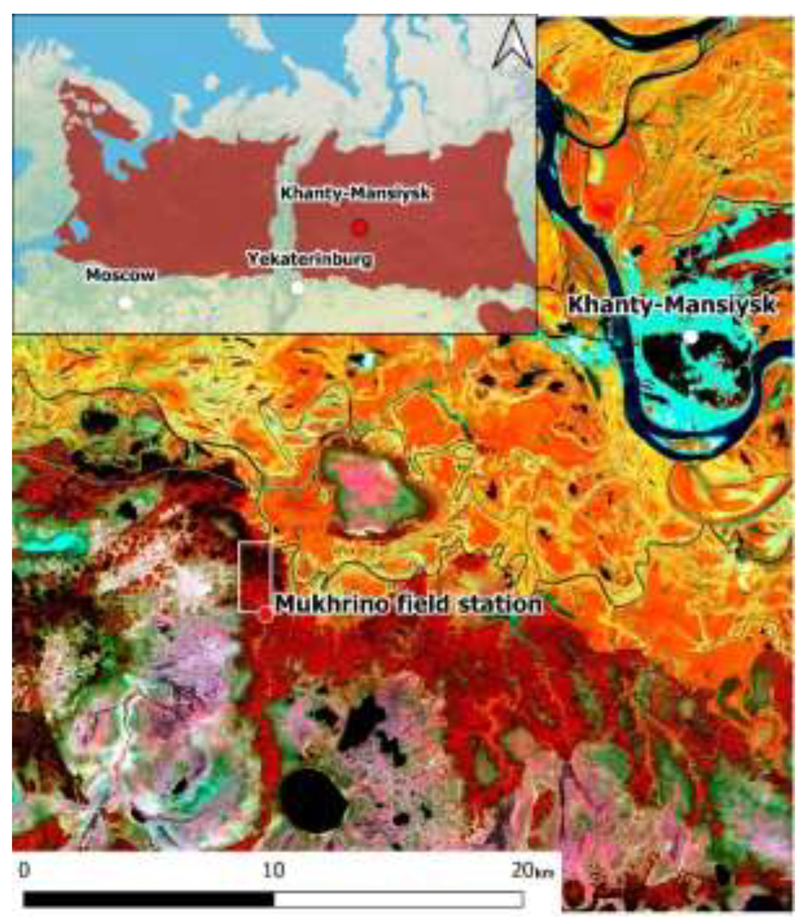
Figure 2.
Relationship (red thick line) between tree diameter and height, obtained from field data (dots). Thin lines show the range of model errors.
Figure 2.
Relationship (red thick line) between tree diameter and height, obtained from field data (dots). Thin lines show the range of model errors.
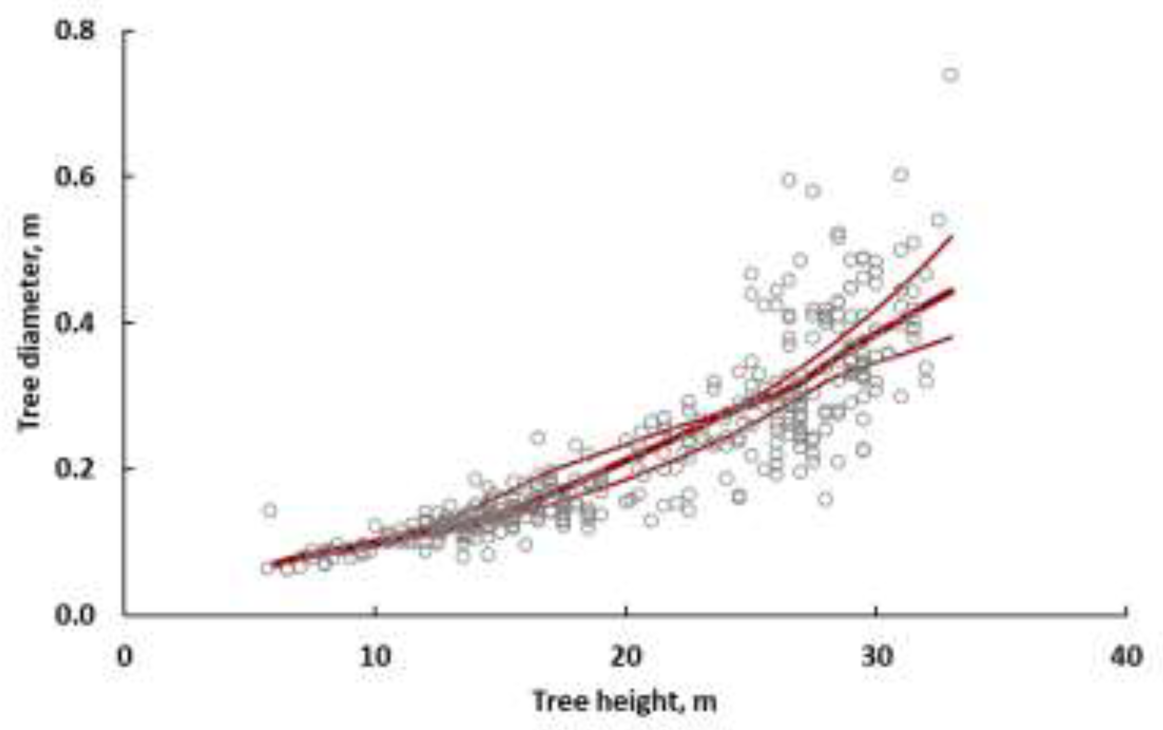
Figure 3.
Relationship between (a) the number of overstory trees on sites 1-5 obtained by ground-based forest inventory and LiDAR survey; (b) all trees (overstory and understory) trees obtained by ground-based forest inventory on these sites and LiDAR survey.
Figure 3.
Relationship between (a) the number of overstory trees on sites 1-5 obtained by ground-based forest inventory and LiDAR survey; (b) all trees (overstory and understory) trees obtained by ground-based forest inventory on these sites and LiDAR survey.
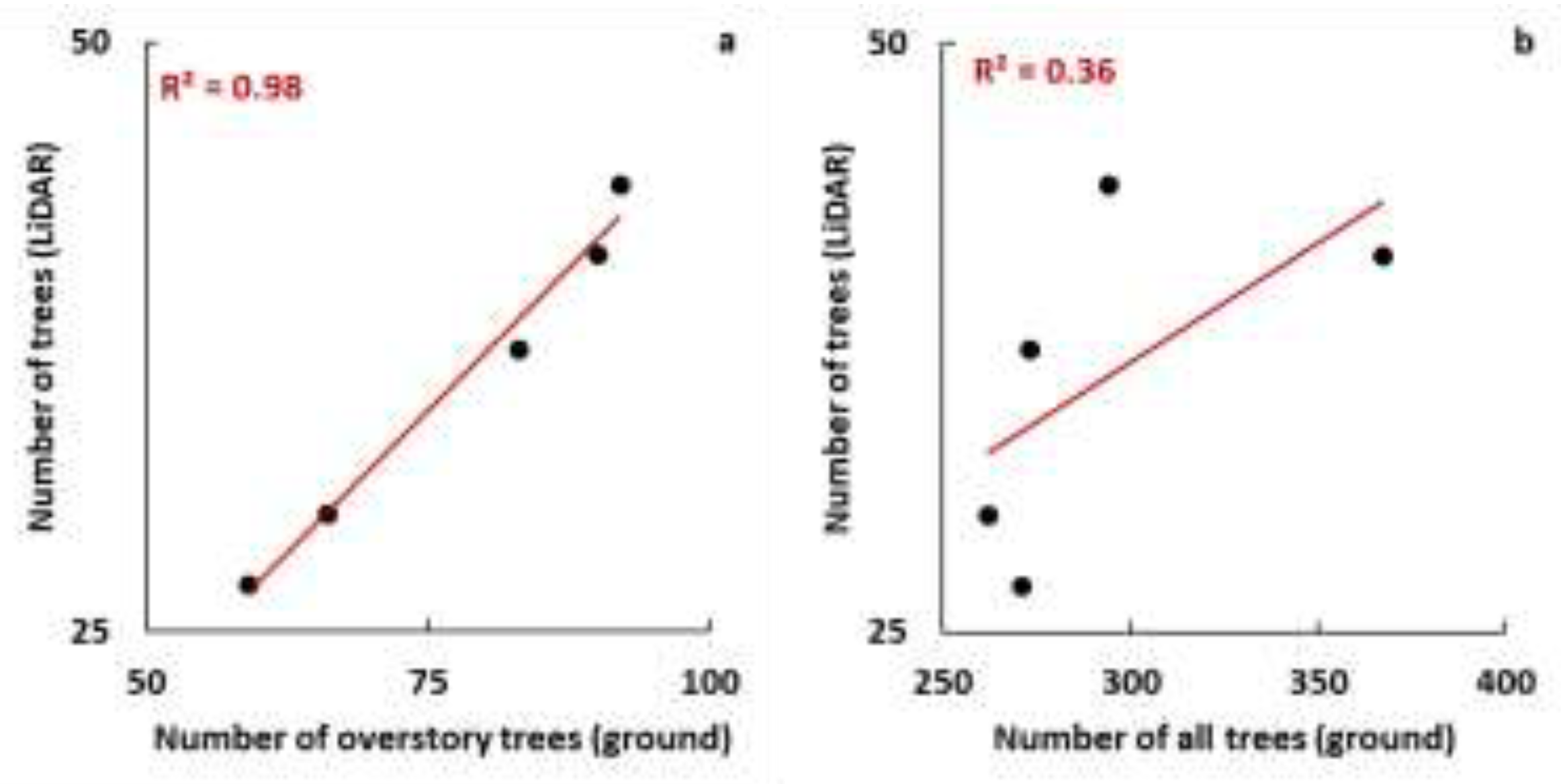
Figure 4.
Boxplot of tree heights obtained (from left to right) using ground data, ground data for overstory trees only, and LiDAR data on sites 1–5. p shows the probability of the null hypothesis about differences between samples, obtained using the Mann–Whitney U-test.
Figure 4.
Boxplot of tree heights obtained (from left to right) using ground data, ground data for overstory trees only, and LiDAR data on sites 1–5. p shows the probability of the null hypothesis about differences between samples, obtained using the Mann–Whitney U-test.
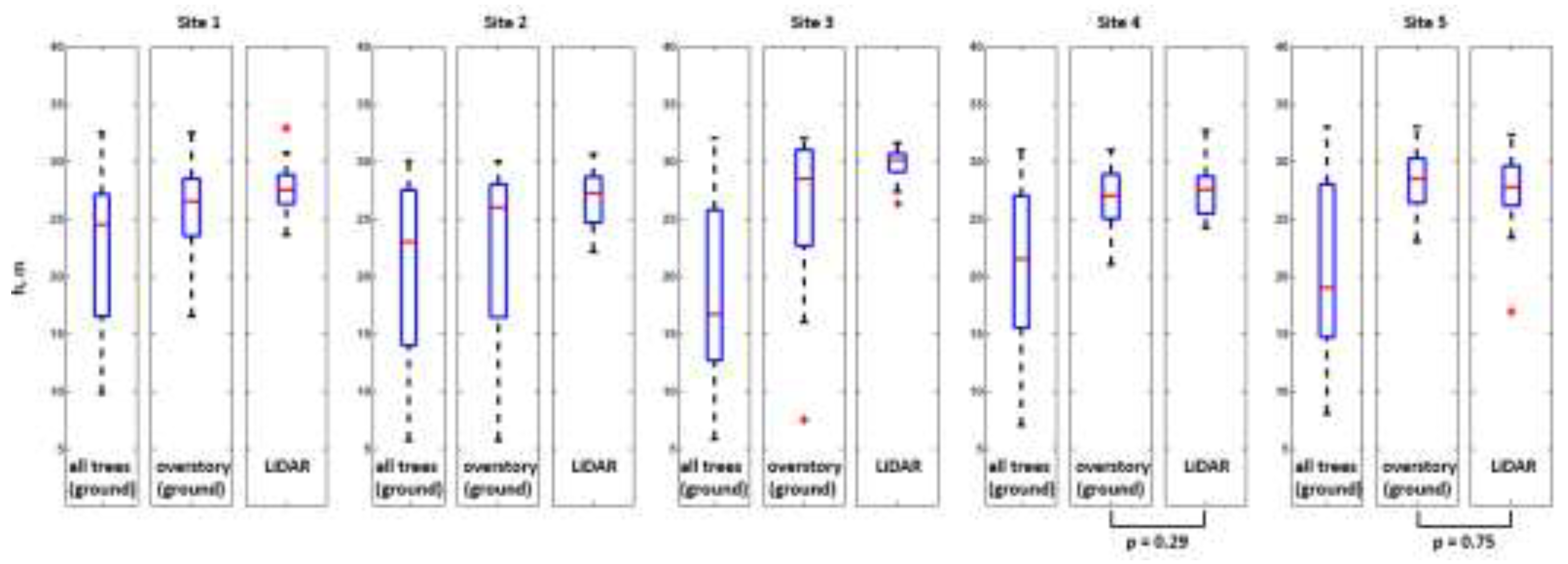
Figure 5.
Boxplot of tree diameters obtained (from left to right) using ground data, ground data for overstory trees only, and LiDAR data on sites 1–5. p shows the probability of the null hypothesis about differences between samples, obtained using the Mann–Whitney U-test.
Figure 5.
Boxplot of tree diameters obtained (from left to right) using ground data, ground data for overstory trees only, and LiDAR data on sites 1–5. p shows the probability of the null hypothesis about differences between samples, obtained using the Mann–Whitney U-test.
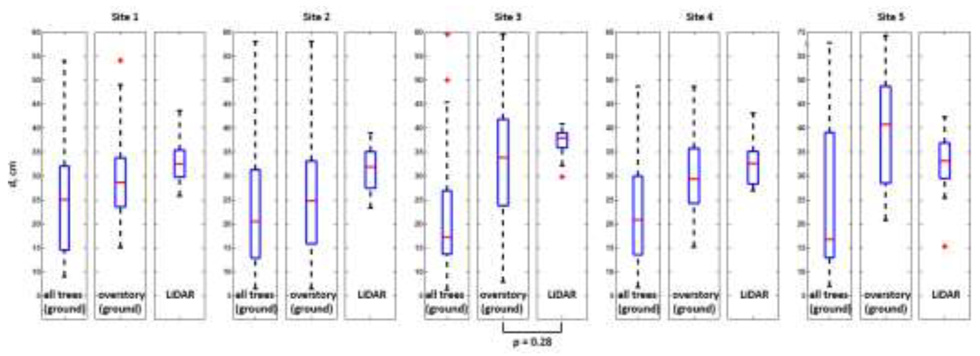
Figure 6.
Relationship between AGB of trees on sites 1-5 obtained by ground-based forest inventory and LiDAR survey.
Figure 6.
Relationship between AGB of trees on sites 1-5 obtained by ground-based forest inventory and LiDAR survey.
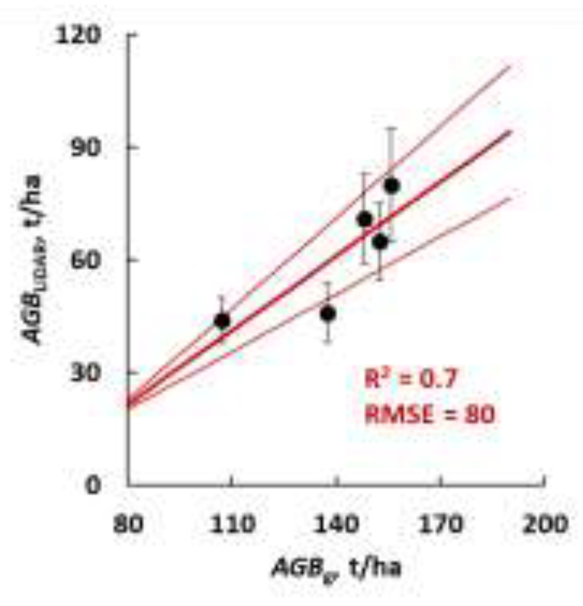
Figure 7.
Relationship between AGB of trees on sites 1-5 obtained by ground-based forest inventory and corrected LiDAR assessment.
Figure 7.
Relationship between AGB of trees on sites 1-5 obtained by ground-based forest inventory and corrected LiDAR assessment.
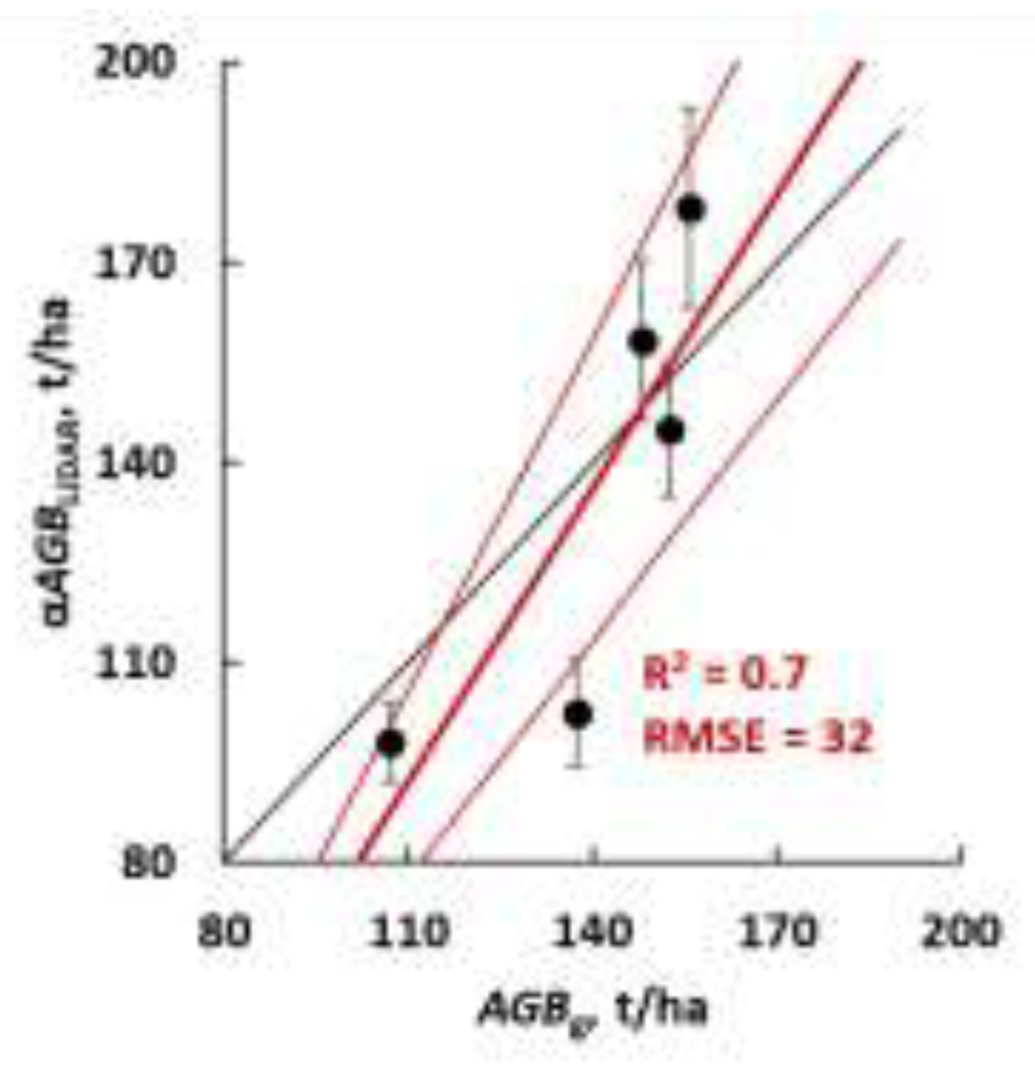
Figure 8.
AGB of trees in mixed forest, obtained by ground-based forest inventory and corrected LiDAR assessment.
Figure 8.
AGB of trees in mixed forest, obtained by ground-based forest inventory and corrected LiDAR assessment.
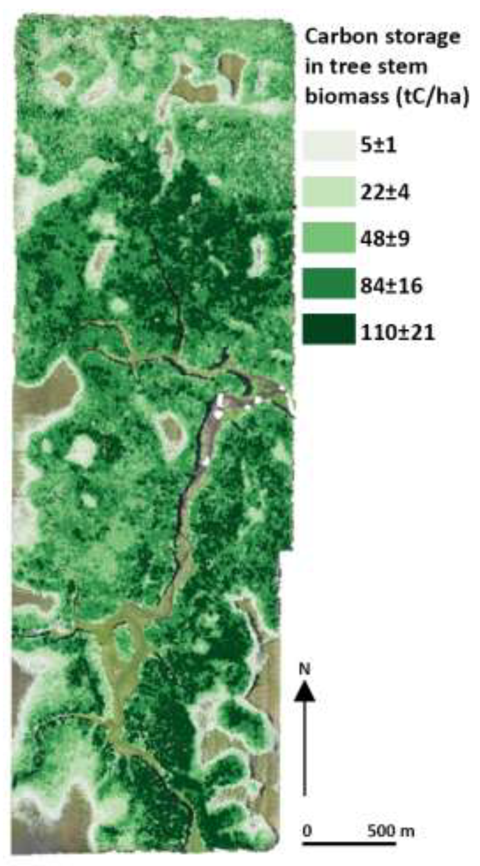

Table 1.
Geographical coordinates of forest taxation sites
| Sites ID | Longitude | Latitude | Area, ha |
| 1 | 60.89435 N | 68.70799 E | 0.25 |
| 2 | 60.89372 N | 68.71013 E | 0.25 |
| 3 | 60.89452 N | 68.71229 E | 0.25 |
| 4 | 60.89556 N | 68.70989 E | 0.25 |
| 5 | 60.89747 N | 68.71014 E | 0.25 |
Table 2.
Identified parameters of allometric models.
| Parameter | Value | Error |
| a | 4.9 × 10⁻² | 0.2 × 10⁻² |
| b | 6.9 × 10⁻² | 0.1 × 10⁻² |
| c | 0.3× 10⁻² | 0.2 × 10⁻³ |
| d | 148.1 × 10⁻² | 2.9 × 10⁻² |
| e | 1.2 × 10⁻² | 0.7 × 10⁻⁴ |
Table 3.
Carbon storage in forests according to literature data
| C, t/ha | Dominant tree | Country | Reference |
| 81–260 | Pinus sylvestris | Finland | [37] |
| 57 | Pinus sylvestris | Norway | [38] |
| 92 | Picea abies | Norway | [38] |
| 51 | Pinus sylvestris | Canada | [38] |
| 87–146 | Pinus sylvestris | Sweden | [39] |
| 38–143 | Pinus resinosa, Populus spp. | USA | [40] |
| 40–66 | Picea abies | Norway | [41] |
| 40–80 | Betula pendula, Betula platyphylla, Populus tremula | Mongolia | [42] |
| 42–137 | Betulaspp. | China | [43] |
| 48–110 | Populus tremula, Betula pubescens, Pinus sibirica, Abies sibirica, Picea obovata | Russia | Current study (well-drained parts) |
| 54 | Current study (mean) | ||
| 83 | - | - | Mean all studies |
Disclaimer/Publisher’s Note: The statements, opinions and data contained in all publications are solely those of the individual author(s) and contributor(s) and not of MDPI and/or the editor(s). MDPI and/or the editor(s) disclaim responsibility for any injury to people or property resulting from any ideas, methods, instructions or products referred to in the content. |
© 2024 by the authors. Licensee MDPI, Basel, Switzerland. This article is an open access article distributed under the terms and conditions of the Creative Commons Attribution (CC BY) license (https://creativecommons.org/licenses/by/4.0/).
Copyright: This open access article is published under a Creative Commons CC BY 4.0 license, which permit the free download, distribution, and reuse, provided that the author and preprint are cited in any reuse.


