
Submitted:
22 November 2024
Posted:
26 November 2024
You are already at the latest version
Abstract
Managing forecast risk is key during the treasury management process. The entire treasury management process [8] is moving into the future and is therefore based on the prediction of future free cash flows discounted at the cost of capital. We used both numerical method and analytical method to solve veridical type paradoxes. We used Monte Carlo simulation as numerical method. Following analytical methods were used: conditional probability [10], Bayes' rule and Bayes' rule with multiple conditions. We successfully solved all the veridical type paradoxes and discovered why such a big discussion of Monty Hall problem appeared in 90s. We varied Monty Hall problem, using different doors count and prizes count.
Keywords:
Treasury Management
; Monte Carlo simulation
; managing forecasting risk
; Bertrand's box paradox
; three prisoners' dilemma
; Monty Hall problem
; Bayes' rule
; Byes' rule with multiple conditions
; conditio
1. Introduction
A very useful one for forecast risk management is the Monte-Carlo method. It is not as popular as forecast risk management based on sensitivity analysis, either threshold point analysis or sensitivity analysis or decision tree analysis. Its limitation has sometimes been veridical type paradoxes. Our article goes beyond this barrier. A paradox is a statement that contradicts itself and yet might be true (or wrong at the same time).
A paradox is a statement that contradicts itself and yet can be true (or false at the same time). A verifiable paradox produces a result that seems absurd, but nevertheless turns out to be true. We will focus on verifiable-type paradoxes using Monte Carlo simulations, but will also present analytical solutions for most cases (Carsey, Harden, 2014), (Austin, 2009a). A key part of our useful treasury management research (Arnold, Yildiz, 2015) in forecast risk management has been the Monty Hall problem, and we will use Monte Carlo simulations for all calculations in this case, but we will also provide analytical solutions for most cases. We will describe and solve the following truth-type paradoxes: Bertrands box paradox, Three prisoners dilemma, Monty Hall problem. A key part of our research was the Monty Hall problem, and we will explain why so many Treasury Management researchers insisted on a probability of 0.5 back in the 1990s.
2. Monte Carlo Simulation in Treasury Management
Treasury Management is conducted under conditions of uncertainty and risk. Since risk is a situation in which one or more of the elements that make up the conditions under which a decision is made are unknown, but the probability of that unknown element is known, there is room for using the Monte-Carlo method to manage forecast risk (Pereira, Pinho, Galhardo, Macêdo, 2014). If this probability were not known, we would be dealing with uncertainty. As with the use of Monte-Carlo to manage forecast risk during Treasury Management, risk conditions can only be spoken of if known past experience of analogous events can be compared with the current situation.
Decision problems occurring in risk conditions can be solved using probability calculus or statistical methods (Vithayasrichareon, MacGill, 2012). Monte Carlo simulation is among the advanced statistical tools used in Treasury Management forecast risk management. A simulation is an experiment (Arnold, Yildiz, 2015), usually conducted on a computer, involving the use of random numbers. A stream of random numbers is a sequence of statistically independent random variables uniformly distributed, usually in the interval [0,1).
Simulations are used where it is difficult to use purely analytical methods to model the real situation or to solve basic mathematical problems. They involve repeated random sampling to produce numerical results. We used random sampling to get a probability approximation.
Treasury Management that takes risk management into account, reduces the volatility of cash flows (Hong, Hu, Liu, 2014), and thus increases the value of the company. This is because, as the risk associated with an enterprise increases, capital providers demand a higher interest rate. Entities with lower risk, have the possibility of preferential treatment by counterparties. Both by suppliers of materials, goods and services and by suppliers of capital. Such preferential treatment will lower the cost of capital financing the company and thus increase the company's Treasury value. Risk-adjusted Treasury Management increases the value of the enterprise (Fantazzini, 2009), as the probability of the entity going bankrupt is then reduced (Hong, Hu, Liu, 2014). As a result, the company will operate for a longer period of time and will therefore generate positive free cash flows for a longer period of time, thereby increasing the Corporate Treasury.
The Monte-Carlo analysis method is considered a method of forecast risk management in Corporate Treasury Management, indirectly taking into account the risk of error in the forecast made (Austin, 2009a), (Austin, 2009b). Together with scenario analysis, it is an indirectly risk-adjusted method for analyzing the risks of Corporate Treasury Management carried out under conditions of uncertainty and risk.
Similarly, in the Monte-Carlo method, for each Corporate Treasury Management decision, forecasts are made of the development of factors affecting the value of Treasury growth under various future development scenarios (Fantazzini, 2009). The application of Monte-Carlo analysis should show whether the Corporate Treasury Management measure being evaluated should not be implemented by the company, since the expected value of Treasury growth is a key parameter in this procedure.
Monte-Carlo analysis has an informational advantage over sensitivity analysis. It is used to analyze Corporate Treasury Management under risk and uncertainty by examining the sensitivity of Treasury protection, creation and accumulation to changes in single factors. Monte-Carlo analysis is, in a sense, an extension of decision tree analysis, which is applicable when the Corporate Treasury Management process under analysis consists of a sequence of decisions and when decisions made at subsequent moments depend on the results of previous decisions.
Monte Carlo simulation) is a type of analysis associated with sensitivity analysis enriched with probability distributions of explanatory variables. It involves the use of pseudo-random number generators to mimic the time course of cash flows that will occur in a company (Brandimarte, 2014). Like scenario analysis, it estimates the expected value of creation, protection or accumulation of Treasury (Alban, Darji, Imamura, Nakayama, 2017), measures of risk and other parameters, and is considered a more accurate method. Monte-Carlo analysis is carried out on the basis of a mathematical model describing treasury management (Koller, Friedman, 2009). The first step in its application in Corporate Treasury Management is to create a model containing the company's free cash flow FCF. After determining the probability distributions of each random variable, the simulation software makes a random selection of each variable (Page, 2010). The selected value of each random variable, along with the specified values of certain variables, is then used to determine the expected cash flows. Such a process is repeated several times, and each time specific results are obtained, which are used to construct the probability distribution, its expected value and standard deviation (Batan, Graff, Bradley, 2016). The final result of the Monte Carlo analysis is, as in scenario analysis and decision tree analysis, the expected net present value, on the basis of which the company can decide to accept or reject the implementation of a Treasury Management project (Steffen, 2018) whose risk effectiveness is analyzed based on this method (Page, 2010).
In the process of evaluating Corporate Treasury Management undertaken under conditions of risk (Pereira, Pinho, Galhardo, Macêdo, 2014), in addition to methods that indirectly take into account risk (Vithayasrichareon, MacGill, 2012), Monte Carlo simulation is preferred, as well as measures that assess the effectiveness of the activity that is the subject of Treasury Management's decision based on the coefficient of variation or based on the modification of measures by adjustments due to the need to take into account risk (Pereira, Pinho, Galhardo, Macêdo, 2014).
The coefficient of variation is a measure of risk, indicating what level of risk is per unit of financial parameter (Rajesh, Preethi, Kavitha, Gunasekaran, Kumar, 2020). If the coefficient of variation is used, priority in implementation should be given to Treasury Management measures whose results have a lower coefficient of variation. Monte-Carlo simulation avoids the simplistic generalizations implied by the coefficient of variation (Brandimarte, 2014).
3. Veridical Type Paradoxes
We will solve following veridical type paradoxes: Bertrand's box, Three prisoner's dilemma and Monty Hall problem.
We solved following veridical type paradoxes: Bertrands box, Three prisoners dilemma and Monty Hall problem. We used both analytical and numerical approach. Some calculations were conducted just numerically.
3.1. Bertrand’s box
Bertrands box paradox is a paradox of elementary probability theory (Batan, Graff, Bradley, 2016). There are three boxes:
- A box containing two gold coins
- A box containing two silver coins
- A box containing one gold coin and a silver coin
The question is: What is the probability of choosing gold coin, having known the first coin is also gold? Player is choosing box at random and does not swap boxes after first toss. It is an elementary example of conditional probability:
$$P(A\mid B)={P(A\cap B)\over{P(B)}}$$
- P(A) – probability of choosing gold coin in second toss
- P(B) – probability of choosing gold coin in first toss
$$P(B)={1+0+{1\over2}\over3}={1\over2 }$$
$$P(A\cap B)={1\over 3}$$
$$P(A\mid B)={{1\over 3}\over{1\over 2}}={2\over 3}$$
Result appears to be $1\over2$ using common sense, but it is $2\over3$ in fact. The correct solution of the problem is well known for a long time. The aim of our research was to build a Monte Carlo simulation of the problem. We coded following code in R:
- [
- basicstyle=\small,
- ]
- #Bertrand's paradox
- set.seed(100)
- samplesize<-1000000
- a<-sample(0:2,samplesize,replace=T)
- # 3 boxes: 0- gold, gold; 1 - silver, silver; 2 - gold, silver
- b<-sample(0:1,samplesize,replace=T) # 2 balls in each box
- data<-data.frame(a,b)
- data2<-subset(data,(a==0) | (a==2 & b==0),select=a)
- round(sum(a==0)/nrow(data2),4) # final probability
Monte Carlo simulation confirms the probability equal 0.6667, which is $2\over3$.
3.2. Three prisoners dilemma
Three prisoners problem is another veridical type paradox. Three prisoners A,B and C, are in separate cells and sentenced to death. The governor has selected one of them at random to be pardoned. The warden knows which one is pardoned, but is not allowed to tell. Prisoner A begs the warden to let him know the identity of the lucky one. Prisoner A knows that warden cant tell the identity of the one to be pardoned, so he proposed the warden following code : If B is pardoned, give me Cs name. If C is pardoned give me Bs name. If I am pardoned, flip a coin to decide whether to name B or C. The warden tells A that it will be B. Prisoner A is pleased because he believes that his probability of surviving has gone up from $1\over3$ to $1\over2$, as it is now between him and C. This is what common sense says. The question is, what the true probabilities are. Analytical solution:
- A,B,C are corresponding prisoners
- P(A),P(B),P(C) are probabilities that governor pardoned corresponding prisoners
- a,b,c are events which warden mentions that corresponding prisoners were pardoned
$$P(A)=P(B)=P(C)={1\over3}, P(b\mid A)={1\over2}, P(c\mid A)={1\over2}$$
It is more complicated problem. It can be solved using Bayes rule.
$$P(A\mid b)={{P(b\mid A)P(A)}\over {P(b\mid A)P(A)+P(b\mid B)P(B)+P(b\mid C)P(C)}}$$
$$P(A\mid b)={{{1\over2}.{1\over3}}\over {{1\over 2}.{1\over 3}+0.{1\over 3}+1.{1\over 3}}}={{1\over 6}\over {1\over 2}}={1\over 3}$$
$$P(A\mid c)={{P(c\mid A)P(A)}\over {P(c\mid A)P(A)+P(c\mid B)P(B)+P(c\mid C)P(C)}}$$
$$P(A\mid c)={{{1\over2}.{1\over3}}\over {{1\over 2}.{1\over 3}+1.{1\over 3}+0.{1\over 3}}}={{1\over 6}\over {1\over 2}}={1\over 3}$$
$$P(C\mid b)={{P(b\mid C)P(C)}\over {P(b\mid A)P(A)+P(b\mid B)P(B)+P(b\mid C)P(C)}}$$
$$P(C\mid b)={{1.{1\over3}}\over {{1\over 2}.{1\over 3}+0.{1\over 3}+1.{1\over 3}}}={{1\over 3}\over {1\over 2}}={2\over 3}$$
Conclusion of three prisoners problem is, that wardens information is not telling anything about prisoner A future. Probability of being pardoned stays at $1\over 3$. Probability of being pardoned for prisoner C is now $2\over 3$. Monte Carlo simulation has been coded in R:
- [
- basicstyle=\small,
- ]
- # Three prisoners problem
- set.seed(100)
- samplesize<-1000000
- governor<-sample(0:2,samplesize,replace=T)
- fm<-function(a,j) {
- if (a[j]==0) {thisone<-sample(1:2,1,replace=T)}
- if (a[j]==1) {thisone<-2}
- if (a[j]==2) {thisone<-1}
- thisone
- }
- warden<- sapply(1:samplesize, function(j) fm(governor,j))
- r<-data.frame(governor,warden)
- # Warden told B, given governor choose A.
- sum(r$warden==1 & r$governor==0)/sum(r$warden==1)
- # Warden told C, given governor choose A.
- sum(r$warden==2 & r$governor==0)/sum(r$warden==2)
- # Warden told B, given governor choose C.
- sum(r$warden==1 & r$governor==2)/sum(r$warden==1)
- # Warden told C, given governor choose B.
- sum(r$warden==2 & r$governor==1)/sum(r$warden==2)
Monte Carlo simulations provide the same results as analytical solution provides: 0.3335 and 0.6665.
3.3. Monty Hall problem
Monty Hall problem was the key part of our research. We will try to explain the discussion of the problem back in 90s (Austin, 2009b). Suppose you are on a game show, and you are given the choice of three doors: Behind one door is a car; behind the others, goats. You pick a door, say No. 1, and the host, who knows what is behind the doors, opens another door, say No. 3, which has a goat. He then says to you, "Do you want to pick door No. 2?" Is it to your advantage to switch your choice? Common sense tells that whether you switch your choice or not, you still have 50 per cent chance to win. Analytical solution of Monty Hall problem for three doors is :
- Events C1,C2,C3, are indicating the car is behind door 1,2 or 3.
- $P(C_1 )=P(C_2 )=P(C_3 )={1\over 3}$
- Event X1 is indicating player initialy choosing door 1.
- As the position of the car is independent of the player’s first choice $P(C_i |X_1 )={1\over3}$.
- H3 is host opening door 3.
Following probabilities are obvious :
$$P(H_3\mid C_1,X_1 )={1\over2},P(H_3\mid C_2,X_1 )=1,P(H_3\mid C_3,X_1 )=0$$
Probability that car is behind door No. 2, given player initialy choosing door 1 and host opening door No. 3 is :
$$P(C_2\mid H_3,X_1 )={{P(H_3\mid C_2,X_1 )P(C_2 |X_1 )}\over {P(H_3\mid X_1 )}}$$
$$\footnotesize{ \begin{multlined} P(C_2\mid H_3,X_1 )= \\ ={{P(H_3\mid C_2,X_1 )P(C_2\mid X_1 )}\over{P(H_3\mid C_1,X_1)P(C_1\mid X_1 )+P(H_3\mid C_2,X_1)P(C_2\mid X_1)+P(H_3\mid C_3,X_1)P(C_3 |X_1 )}} \end{multlined} }$$
$$P(C_2|H_3,X_1)={1.{1\over3}\over{{1\over2}×{1\over3}+1.{1\over3}+0.{1\over3}}}={2\over3}$$
Probability that car is behind door No.1, given player initially choosing door No. 1 and host opening door No. 3 is :
$$P(C_1 |H_3,X_1 )={{(H_3 |C_1,X_1 )P(C_1 |X_1 )}\over{P(H_3 |X_1 )}}$$
$$\footnotesize{ \begin{multlined} P(C_1\mid H_3,X_1 )=\\ ={{P(H_3\mid C_1,X_1 )P(C_1\mid X_1 )}\over{P(H_3\mid C_1,X_1)P(C_1\mid X_1 )+P(H_3\mid C_2,X_1)P(C_2\mid X_1)+P(H_3 \mid C_3,X_1)P(C_3\mid X_1)}} \end{multlined} }$$
$$P(C_1|H_3,X_1)={{1\over2}{1\over3}\over{{1\over2}×{1\over3}+1.{1\over3}+0.{1\over3}}}={1\over3}$$
Flip a coin decision has following probability :
$$P(flip\ a\ coin)={1\over2}P(C_1 |H_3,X_1 )+{1\over2}P(C_2|H_3,X_1)$$
$$P(flip\ a\ coin)={1\over2}{1\over3}+{1\over2}{2\over3}={1\over2}$$
Analytical solution shows that player should switch her choice, since chance to win is ${2\over3}$. In case player does not switch her choice, chance to win is just ${1\over3}$. We used Bayes rule with multiple conditions. Flip a coin decision probability is equal to ${1\over2}$. Since Monty Hall problem is key part of our research, we have focused on many different decisions (Vithayasrichareon, MacGill, 2012), which were simulated in Monte Carlo simulations. We explored following cases (Carsey, Harden, 2014), (Koller, Friedman, 2009):
Not switching decision
- 1)
- Switching decision
- 2)
- Flip a coin decision
- 3)
- Tic-toc decision
- 4)
- Opposite tic-toc decision
We coded simulations which vary doors count and also prizes count. If contestant decides to switch door, and there is more than one door available, she will choose another door randomly. If contestant flips a coin, she does it just once. If there is more just one door available, she will choose another door randomly, too. Following code simulates different doors count and also cars count options. Code has been written in R:
- [
- basicstyle=\small,
- ]
- #Monty Hall problem
- samplesize<-100000 # sample size
- doors<-9 # doors count -1
- door<-vector("numeric",length=doors*(doors-1)/2)
- prize<-vector("numeric",length=doors*(doors-1)/2)
- changedp<-vector("numeric",length=doors*(doors-1)/2)
- nochangep<-vector("numeric",length=doors*(doors-1)/2)
- ttp<-vector("numeric",length=doors*(doors-1)/2)
- ottp<-vector("numeric",length=doors*(doors-1)/2)
- flipp<-vector("numeric",length=doors*(doors-1)/2)
- results <- data.frame(door, prize, changedp, ttp,flipp,
- ottp,nochangep)
- #tic-toc oppposite tic-toc function
- ttott<-function(ttott1,win1,win2,trigger){
- if (ttott1==0) {if (win2==0) {thisone<-0
- } else {thisone<-1 }}
- if (ttott1==1) {if (win1==0) {thisone<-1
- } else {thisone<-0 }}
- if (trigger=="ott") {if (thisone==0) {thisone<-1
- } else {thisone<-0 }}
- thisone}
- for (i in 2:doors) {
- for (j in 1:(i-1)) {
- set.seed(100)
- initial<-replicate(samplesize,list(sample(0:i,1,replace=F)))
- priz<-replicate(samplesize,list(sample(0:i,j,replace=F)))
- # initial guess & prizes behind doors
- flip<-sample(0:1,samplesize, replace=T) # flip a coin
- tt<-sample(0,samplesize,replace=T) # tic toc
- ott<-sample(0,samplesize,replace=T) # opposite tic toc
- choices<-replicate(samplesize,list(c(0:i)))
- # WHICH GOAT WILL BE SHOWN
- goats<-mapply(setdiff,choices,priz)
- goats2<- lapply(1:ncol(goats), function(p) goats[,p])
- # goats are opposite prizes
- notinitial<-mapply(setdiff,choices,initial)
- notinitial2<-lapply(1:ncol(notinitial),
- function(p) notinitial[,p])
- # group of not initial decisions
- goats3<-mapply(intersect,goats2,notinitial2)
- goats4<-lapply(goats3, function(p) c(p,p))
- goat<-lapply(goats4, function(p) sample(p,1))
- # to show just one goat from intersect not initial & goats
- remove(goats,goats2,choices,notinitial,goats3,goats4)
- chmind<-mapply(setdiff,notinitial2,goat)#to change mind
- #to exclude goat which was shown from not initial group
- if (is.null(ncol(chmind))==FALSE) {
- chmind2<- lapply(1:ncol(chmind), function(p) chmind[,p])
- } else {chmind2<-chmind }
- chmind3<-lapply(chmind2, function(p) c(p,p))
- newmind<-lapply(chmind3, function(p) sample(p,1))
- # to choose 1 new decision from all the available
- remove(notinitial2, goat,chmind,chmind2,chmind3)
- win1<-mapply(intersect,newmind,priz)#win1 changed mind
- win2<-mapply(intersect,initial,priz)#win2 not changed mind
- win13<-as.numeric(lapply(win1,function(p) length(p)==0))
- win23<-as.numeric(lapply(win2, function(p) length(p)==0))
- # intersection - 1 no intersection,0 intersection
- for(l in 1:(samplesize-1)) { # TIC-TOC, OPPOSITE TIC TOC
- tt[l+1]<-ttott(tt[l],win13[l],win23[l],'tt')
- ott[l+1]<-ttott(ott[l],win13[l],win23[l],'ott')}
- #PROBABILITIES
- win1p<-sum(win13==0)/samplesize #win1p changed mind
- win2p<-sum(win23==0)/samplesize #win2p not changed mind
- remove(newmind,priz,initial,win1,win2)
- flipfr<-data.frame(win13,win23,flip,tt,ott)
- flip1<-nrow(flipfr[flipfr$flip==1 & flipfr$win13==0,])
- flip2<-nrow(flipfr[flipfr$flip==0 & flipfr$win23==0,])
- # flip1 - changed mind,flip2 - initial decision
- tt1<-nrow(flipfr[flipfr$tt==1 & flipfr$win13==0,])
- tt2<-nrow(flipfr[flipfr$tt==0 & flipfr$win23==0,])
- ott1<-nrow(flipfr[flipfr$ott==1 & flipfr$win13==0,])
- ott2<-nrow(flipfr[flipfr$ott==0 & flipfr$win23==0,])
- flipp<-(flip1+flip2)/samplesize
- tictocp<-(tt1+tt2)/samplesize
- opptictocp<-(ott1+ott2)/samplesize
- results$door[i*(i-1)/2-i+1+j]<-i+1#RESULTS - WRITTING
- results$prize[i*(i-1)/2-i+1+j]<-j
- results$changedp[i*(i-1)/2-i+1+j]<-round(win1p*100,3)
- results$ttp[i*(i-1)/2-i+1+j]<-round(tictocp*100,3)
- results$flipp[i*(i-1)/2-i+1+j]<-round(flipp*100,3)
- results$ottp[i*(i-1)/2-i+1+j]<-round(opptictocp*100,3)
- results$nochangep[i*(i-1)/2-i+1+j]<-round(win2p*100,3)
- remove(win13,win23,flipfr,flip,tt,ott) } }
- nname<- paste(toString(samplesize),"r.txt",sep="")
- write.table(results,nname,append=FALSE)
Table 1 shows output of the code. Probabilities were calculated with sample size equal 1,5 million. Probability theory allows a simple derivation of Monte Carlo simulations error. If contestant does not change her mind, probability of winning is a very simple formula.
$$P(not\ switching\ decision)={prizes\ count\over doors\ count}$$
We can measure Mean Absolute Error of Monte Carlo simulations probabilities for not switching decision and Bias.
$$MAE={1\over 36}\sum_{i=1}^{36} \mid {p_{MC}}_i-p_{{true}_i}\mid = {0.933\over 36}=0.026$$
$$Bias={1\over 36}\sum_{i=1}^{36} (p_{{MC}_i}-p_{{true}_i}) = {-0.191\over 36}=-0.005$$
Mean Absolute Error is 0.026 per cent, and Bias is -0.005 per cent. These figures are also approximations of Monte Carlo simulations error and Bias for whole Table 1.
Taking the true probabilities for not switching decision into account, we can also reestimate flip a coin decision probabilities. They are in combined column for that decision.
$$P(flip\ a\ coin)={1\over2}P(switching_{Monte\ Carlo})+{1\over2}P(no\ switch_{true})$$
Mean Absulute Error and Bias for this modification of flip a coin decision are:
$$MAE_{modified}={1\over 36}\sum_{i=1}^{36} \mid {p_{MC}}_i-p_{{true}_i}\mid$$
$$p_{{MC}_i}={1\over2}P(switching_{{Monte\ Carlo}_i})+{1\over2}P(no\ switch_{{true}_i})$$
$$p_{{true}_i}={1\over2}P(switching_{{true}_i})+{1\over2}P(no\ switch_{{true}_i})$$
$$MAE_{modified}={1\over 36}\sum_{i=1}^{36} \mid {1\over2}p_{switching_{{MC}_i}}-{1\over2}p_{switching_{true_i}}\mid$$
Since (24) and (25) are approximations of MAE and Bias for whole Table 1:
$$MAE_{modified}\doteq{1\over2}MAE$$
$$Bias_{modified}\doteq{1\over2}Bias$$
Modified probabilities show Table 2.
Dependence between Mean Absolute Error and sample size in Monty Hall problem, calculated from probabilities obtained from Monte Carlo simulations and exact probabilities, in case contestant does not change her mind.
Dependence between Mean Absolute Error and sample size in Monty Hall problem, calculated from probabilities obtained from Monte Carlo simulations and exact probabilities, in case contestant does not change her mind.
Dependence between Bias and sample size in Monty Hall problem, calculated from probabilities obtained from Monte Carlo simulations and exact probabilities, in case contestant does not change her mind.
Dependence between Bias and sample size in Monty Hall problem, calculated from probabilities obtained from Monte Carlo simulations and exact probabilities, in case contestant does not change her mind.
Changedp column describes probabilities in case player changed her mind. No changep column describes probabilities in case player did not change her mind. Flipp column describes probabilities in case player made flip a coin decision. Ttp column describes probabilities in case player is applying tic-toc decision. Ottp column describes probabilities in case player is applying opposite tic-toc decision.
Table 1 and Table 2 show that changing mind is the best decision. Flip a coin decision probabilities always lie between change mind probabilities and do not change mind probabilities. Flip a coin decision for 3 doors and 1 prize is those 50 per cent, which caused a lot of discussion about the Monty Hall problem. Those 50 per cent is those 50 per cent, what common sense tells that the probability should be. Tic-toc decision is better than flip a coin decision. Opposite tic-toc decision is worse than flip a coin decision, but better than do not change mind decision. If player decides to not change her mind, it is the worst decision ever. Flip a coin decision is the third best decision of five different options, and it confirms the old truth: If you do not know what you should do, make a flip a coin decision and you will not decide bad. Research also showed that people should change their mind, because individuals who do not change their mind have the lowest probability for success. Second worst chance for success have individuals who are speculating too much - opposite tic-toc decision. The best chance for success have individuals who change their minds.
Finally, we can plot dependence between Monte Carlo simulations sample size and Mean Absolute Error as MAE=f(samplesize) and also dependence between Monte Carlo simulations sample size and Bias as Bias = f(samplesize). Dependence show Figure 1 and Figure 2.
Tic-toc strategy is a kind of strategy when player makes decision according to last know decision. If last decision is to change mind and was successful, she will also change mind. If last decision is to change mind and was not successful, she will not change mind. Opposite tic-toc strategy is a kind of strategy when player also makes decision according to last known decision. If last decision is to change mind and was successful, she will not change mind. If last decision is to change mind and was not successful, she will change mind. She will do the opposite, because she is expecting that situation will change in next turn. Another interesting fact is how probabilities are increasing with increasing prices count.
4. Conclusions
We studied truth-type paradoxes using conditional probabilities, Bayes' rule and mainly Monte Carlo simulations. The Monte-Carlo analysis method is considered to be a forecast risk management method in Treasury Management indirectly taking into account the risk of error in the forecast made. Together with scenario analysis, it is an indirectly risk-adjusted method for analysing the risks associated with Corporate Treasury Management carried out under conditions of uncertainty and risk (Hong, Hu, Liu, 2014).
Similarly, in Monte-Carlo, for each Treasury Management decision, forecasts are made of the development of factors influencing the value of Treasury growth under different future scenarios of developments. Using the Monte-Carlo analysis should reveal whether the Treasury Management action being assessed should not be implemented by the company, as the expected value of the Treasury increment is a key parameter in this procedure.
Monte-Carlo analysis is superior in its information to sensitivity analysis. It is used to analyse the Treasury Management of an enterprise under conditions of risk and uncertainty, by examining the sensitivity of the protection, creation and accumulation of Treasury to changes in single factors. Monte-Carlo analysis is, in a sense, an extension of decision tree analysis, which is applicable when the Treasury Management process under analysis consists of a sequence of decisions and when decisions taken at subsequent moments depend on the results of previous decisions.
Monte Carlo simulation) is a type of analysis linked to sensitivity analysis enriched with probability distributions of explanatory variables. It involves using pseudo-random number generators to mimic the time course of the cash flows that will take place in a company. Like scenario analysis, it allows for the estimation of the expected value of the creation, protection or accumulation of corporate Treasury (Alban, Darji, Imamura, Nakayama, 2017), measures of risk, and other parameters, and is considered a more accurate method. Monte-Carlo analysis is performed on the basis of a mathematical model describing Treasury Management. The first step in its application in Treasury Management is to create a model containing the company's free cash flow FCF. After determining the probability distributions of each random variable, the simulation software makes a random selection of each variable. The selected value of each random variable, together with the determined values of certain variables, is then used to determine the expected cash flows. Such a process is repeated several times and each time specific results are obtained, which are used to construct the probability distribution, its expected value and standard deviation. The final result of the Monte Carlo analysis is, as in scenario analysis and decision tree analysis, the expected net present value (Fantazzini, 2009), on the basis of which the company can decide to accept or reject the implementation of a Treasury Management project (Steffen, 2018) whose risk efficiency is analysed on the basis of this method.
In the process of evaluating Corporate Treasury Management undertaken under risk conditions, in addition to methods that take risk into account indirectly, Monte Carlo simulation is preferable to coefficient of variation-based measures assessing the effectiveness of an action that is the subject of a Treasury Management decision, or based on the modification of measures by adjustments resulting from the need to take risk into account.
The coefficient of variation is a measure of risk, indicating what level of risk is per unit of financial parameter (Alban, Darji, Imamura, Nakayama, 2017). When using the coefficient of variation, priority for implementation should be given to Treasury Management measures whose results have a lower coefficient of variation. Monte-Carlo simulation avoids the simplistic generalisations implied by the coefficient of variation.
We discovered why much of the discussion of the Monty Hall problem took place in the 1990s and why so many researchers believed that the probability was 50 per cent. This 50 per cent represents the decision to flip a coin. We found that the players should change their minds and this is the best decision of all those studied. If the players do not change their minds, it is the worst decision ever. The second worst decision is the one where the players speculate too much - the opposite tic-toc decision. On the other hand, the right speculation is positive - the tic-tac decision being the second best decision. The study showed a lot about Monty Hall's problem, and also about life. The aim of the study has been fulfilled.
Author Contributions
Conceptualization, M.P. and G.M.; methodology, M.P. and G.M.; software, M.P.; validation, M.P.; formal analysis, M.P.; investigation, M.P.; writing—original draft preparation, M.P. and G.M.; writing—review and editing, M.P. and G.M.; visualization, M.P.; supervision, M.P. and G.M.; project administration, G.M.; funding acquisition, G.M. All authors have read and agreed to the published version of the manuscript.
Funding
The work was carried out with the financial support of the National Science Center. The research is financed from the 2015-2018 science budget as a research project funded by the National Science Center granted under decision number DEC-2014/13/B/HS4/00192 (project number: 2014/13/B/HS4/00192).
Data Availability Statement
Data are contained within the article.
Acknowledgements
The presented work and results are part of a monothematic series on Treasury Management carried out within the framework of the grant entitled: Cash management in small and medium-sized enterprises using the full operational cycle.
Conflicts of Interest
The authors declare no conflict of interest.
References
- Carsey T., J. Harden (2014), Monte Carlo Simulation and Resampling Methods for Social Science, SAGE Publications, London.
- Koller D., N. Friedman (2009), Probabilistic Graphical Models Principles and Techniques, The MIT Press, London.
- Page S. (2010), Diversity and Complexity. Princeton University Press, Woodstock 2010.
- Brandimarte P. (2014), Handbook in Monte Carlo Simulation: Applications in Financial Engineering, Risk Management, and Economics, Handbook in Monte Carlo Simulation: Applications in Financial Engineering, Risk Management, and Economics, pp. 1 - 662. [CrossRef]
- Alban A., Darji H.A., Imamura A., Nakayama M.K. (2017), Efficient Monte Carlo methods for estimating failure probabilities, Reliability Engineering and System Safety, 165, pp. 376 - 394. [CrossRef]
- Austin P.C. (2009), Some methods of propensity-score matching had superior performance to others: results of an empirical investigation and monte carlo simulations, Biometrical Journal, 51 (1), pp. 171 - 184. [CrossRef]
- Austin P.C. (2009), Balance diagnostics for comparing the distribution of baseline covariates between treatment groups in propensity-score matched samples, Statistics in Medicine, 28 (25), pp. 3083 - 3107. [CrossRef]
- Arnold U., Yildiz Ö. (2015), Economic risk analysis of decentralized renewable energy infrastructures - A Monte Carlo Simulation approach, Renewable Energy, 77 (1), pp. 227 - 239. [CrossRef]
- Steffen B. (2018), The importance of project finance for renewable energy projects, Energy Economics, 69, pp. 280 - 294. [CrossRef]
- Batan L.Y., Graff G.D., Bradley T.H. (2016), Techno-economic and Monte Carlo probabilistic analysis of microalgae biofuel production system, Bioresource Technology, 219, pp. 45 - 52. [CrossRef]
- Rajesh Banu J., Preethi, Kavitha S., Gunasekaran M., Kumar G. (2020), Microalgae based biorefinery promoting circular bioeconomy-techno economic and life-cycle analysis, Bioresource Technology, 302, art. no. 122822. [CrossRef]
- Vithayasrichareon P., MacGill I.F. (2012), A Monte Carlo based decision-support tool for assessing generation portfolios in future carbon constrained electricity industries, Energy Policy, 41, pp. 374 - 392. [CrossRef]
- Pereira E.J.S., Pinho J.T., Galhardo M.A.B., Macêdo W.N. (2014), Methodology of risk analysis by Monte Carlo Method applied to power generation with renewable energy, Renewable Energy, 69, pp. 347 - 355. [CrossRef]
- Hong L.J., Hu Z., Liu G. (2014), Monte carlo methods for value-at-risk and conditional value-at-risk: A review, ACM Transactions on Modeling and Computer Simulation, 24 (4), art. no. 5. [CrossRef]
- Fantazzini D. (2009), The effects of misspecified marginals and copulas on computing the value at risk: A Monte Carlo study, Computational Statistics and Data Analysis, 53 (6), pp. 2168 - 2188. [CrossRef]
Figure 1.
Mean absolute error Monte-Carlo simulations.
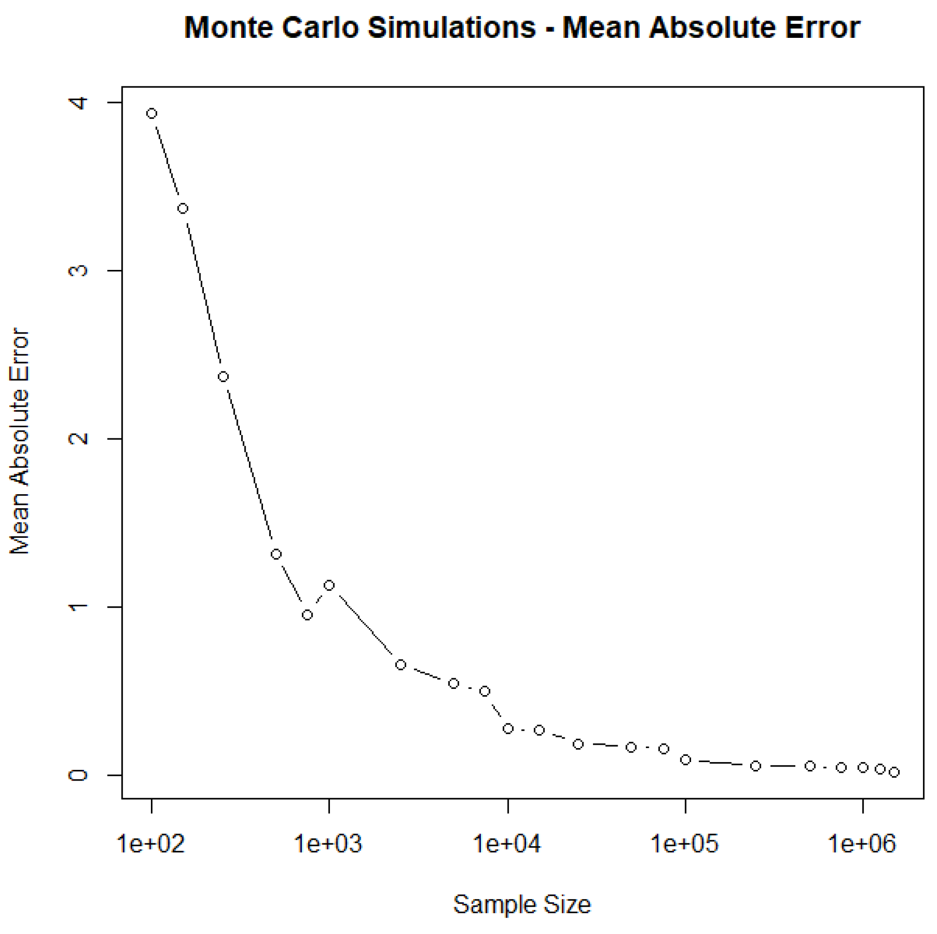
Figure 2.
Bias of Monte-Carlo Simulations.
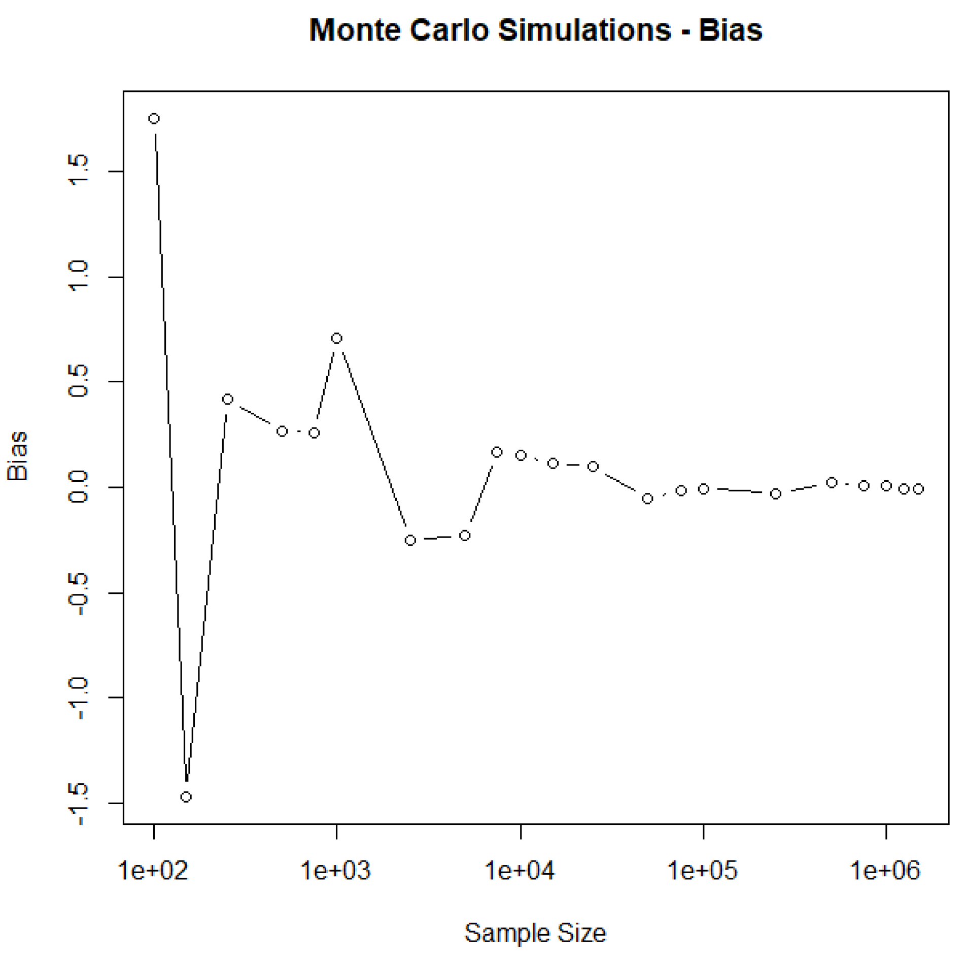

Table 1.
Output of the code. Simulations results.
| No | Door | Prize | Changep | Ttp | Flipp | Ottp | No changep |
|---|---|---|---|---|---|---|---|
| 1 | 3 | 1 | 66.645 | 55.585 | 50.061 | 44.415 | 33.355 |
| 2 | 4 | 1 | 37.545 | 31.857 | 31.278 | 30.005 | 24.992 |
| 3 | 4 | 2 | 75 | 66.686 | 62.54 | 60.013 | 49.993 |
| 4 | 5 | 1 | 26.704 | 23.5 | 23.35 | 22.854 | 19.979 |
| 5 | 5 | 2 | 53.287 | 47.463 | 46.657 | 45.705 | 40.047 |
| 6 | 5 | 3 | 80.014 | 73.354 | 69.997 | 68.534 | 59.99 |
| 7 | 6 | 1 | 20.86 | 18.802 | 18.791 | 18.505 | 16.649 |
| 8 | 6 | 2 | 41.67 | 37.76 | 37.493 | 37.015 | 33.303 |
| 9 | 6 | 3 | 62.565 | 57.244 | 56.253 | 55.6 | 50.053 |
| 10 | 6 | 4 | 83.273 | 77.724 | 75.042 | 74.074 | 66.719 |
| 11 | 7 | 1 | 17.155 | 15.756 | 15.767 | 15.591 | 14.286 |
| 12 | 7 | 2 | 34.268 | 31.582 | 31.477 | 31.138 | 28.581 |
| 13 | 7 | 3 | 51.457 | 47.512 | 47.114 | 46.796 | 42.892 |
| 14 | 7 | 4 | 68.592 | 63.727 | 62.917 | 62.387 | 57.163 |
| 15 | 7 | 5 | 85.661 | 80.856 | 78.553 | 77.89 | 71.399 |
| 16 | 8 | 1 | 14.564 | 13.591 | 13.562 | 13.408 | 12.49 |
| 17 | 8 | 2 | 29.171 | 27.15 | 27.097 | 26.916 | 25.009 |
| 18 | 8 | 3 | 43.77 | 40.764 | 40.609 | 40.408 | 37.492 |
| 19 | 8 | 4 | 58.368 | 54.537 | 54.252 | 53.886 | 49.989 |
| 20 | 8 | 5 | 72.953 | 68.614 | 67.716 | 67.327 | 62.504 |
| 21 | 8 | 6 | 87.511 | 83.353 | 81.251 | 80.743 | 74.955 |
| 22 | 9 | 1 | 12.709 | 11.932 | 11.919 | 11.793 | 11.063 |
| 23 | 9 | 2 | 25.378 | 23.882 | 23.85 | 23.712 | 22.286 |
| 24 | 9 | 3 | 38.05 | 35.79 | 35.62 | 35.541 | 33.302 |
| 25 | 9 | 4 | 50.793 | 47.765 | 47.603 | 47.438 | 44.429 |
| 26 | 9 | 5 | 63.514 | 59.971 | 59.574 | 59.209 | 55.543 |
| 27 | 9 | 6 | 76.224 | 72.26 | 71.459 | 71.043 | 66.624 |
| 28 | 9 | 7 | 88.856 | 85.161 | 83.35 | 82.965 | 77.803 |
| 29 | 10 | 1 | 11.263 | 10.659 | 10.663 | 10.589 | 9.974 |
| 30 | 10 | 2 | 22.496 | 21.287 | 21.273 | 21.272 | 20.021 |
| 31 | 10 | 3 | 33.796 | 31.901 | 31.856 | 31.801 | 29.957 |
| 32 | 10 | 4 | 44.983 | 42.591 | 42.497 | 42.38 | 40.009 |
| 33 | 10 | 5 | 56.281 | 53.328 | 53.151 | 52.905 | 49.971 |
| 34 | 10 | 6 | 67.475 | 64.136 | 63.734 | 63.504 | 59.945 |
| 35 | 10 | 7 | 78.761 | 75.157 | 74.413 | 74.125 | 69.99 |
| 36 | 10 | 8 | 90.008 | 86.636 | 84.967 | 84.669 | 79.949 |
Table 2.
Modified probabilities. Combined results.
| No | Door | Prize | Changep | No changep | No changep | Flipp | Flipp |
|---|---|---|---|---|---|---|---|
| Monte Carlo | True | combined | |||||
| 1 | 3 | 1 | 66.645 | 33.355 | 33.333 | 50.061 | 49.989 |
| 2 | 4 | 1 | 37.545 | 24.992 | 25 | 31.278 | 31.273 |
| 3 | 4 | 2 | 75 | 49.993 | 50 | 62.54 | 62.5 |
| 4 | 5 | 1 | 26.704 | 19.979 | 20 | 23.35 | 23.352 |
| 5 | 5 | 2 | 53.287 | 40.047 | 40 | 46.657 | 46.644 |
| 6 | 5 | 3 | 80.014 | 59.99 | 60 | 69.997 | 70.007 |
| 7 | 6 | 1 | 20.86 | 16.649 | 16.667 | 18.791 | 18.764 |
| 8 | 6 | 2 | 41.67 | 33.303 | 33.333 | 37.493 | 37.502 |
| 9 | 6 | 3 | 62.565 | 50.053 | 50 | 56.253 | 56.283 |
| 10 | 6 | 4 | 83.273 | 66.719 | 66.667 | 75.042 | 74.97 |
| 11 | 7 | 1 | 17.155 | 14.286 | 14.286 | 15.767 | 15.721 |
| 12 | 7 | 2 | 34.268 | 28.581 | 28.571 | 31.477 | 31.42 |
| 13 | 7 | 3 | 51.457 | 42.892 | 42.857 | 47.114 | 47.157 |
| 14 | 7 | 4 | 68.592 | 57.163 | 57.143 | 62.917 | 62.868 |
| 15 | 7 | 5 | 85.661 | 71.399 | 71.429 | 78.553 | 78.545 |
| 16 | 8 | 1 | 14.564 | 12.49 | 12.5 | 13.562 | 13.532 |
| 17 | 8 | 2 | 29.171 | 25.009 | 25 | 27.097 | 27.086 |
| 18 | 8 | 3 | 43.77 | 37.492 | 37.5 | 40.609 | 40.635 |
| 19 | 8 | 4 | 58.368 | 49.989 | 50 | 54.252 | 54.184 |
| 20 | 8 | 5 | 72.953 | 62.504 | 62.5 | 67.716 | 67.727 |
| 21 | 8 | 6 | 87.511 | 74.955 | 75 | 81.251 | 81.256 |
| 22 | 9 | 1 | 12.709 | 11.063 | 11.111 | 11.919 | 11.91 |
| 23 | 9 | 2 | 25.378 | 22.286 | 22.222 | 23.85 | 23.8 |
| 24 | 9 | 3 | 38.05 | 33.302 | 33.333 | 35.62 | 35.692 |
| 25 | 9 | 4 | 50.793 | 44.429 | 44.444 | 47.603 | 47.619 |
| 26 | 9 | 5 | 63.514 | 55.543 | 55.556 | 59.574 | 59.535 |
| 27 | 9 | 6 | 76.224 | 66.624 | 66.667 | 71.459 | 71.446 |
| 28 | 9 | 7 | 88.856 | 77.803 | 77.778 | 83.35 | 83.317 |
| 29 | 10 | 1 | 11.263 | 9.974 | 10 | 10.663 | 10.632 |
| 30 | 10 | 2 | 22.496 | 20.021 | 20 | 21.273 | 21.248 |
| 31 | 10 | 3 | 33.796 | 29.957 | 30 | 31.856 | 31.898 |
| 32 | 10 | 4 | 44.983 | 40.009 | 40 | 42.497 | 42.492 |
| 33 | 10 | 5 | 56.281 | 49.971 | 50 | 53.151 | 53.141 |
| 34 | 10 | 6 | 67.475 | 59.945 | 60 | 63.734 | 63.738 |
| 35 | 10 | 7 | 78.761 | 69.99 | 70 | 74.413 | 74.381 |
| 36 | 10 | 8 | 90.008 | 79.949 | 80 | 84.967 | 85.004 |
Disclaimer/Publisher’s Note: The statements, opinions and data contained in all publications are solely those of the individual author(s) and contributor(s) and not of MDPI and/or the editor(s). MDPI and/or the editor(s) disclaim responsibility for any injury to people or property resulting from any ideas, methods, instructions or products referred to in the content. |
© 2024 by the authors. Licensee MDPI, Basel, Switzerland. This article is an open access article distributed under the terms and conditions of the Creative Commons Attribution (CC BY) license (https://creativecommons.org/licenses/by/4.0/).
Copyright: This open access article is published under a Creative Commons CC BY 4.0 license, which permit the free download, distribution, and reuse, provided that the author and preprint are cited in any reuse.


