
Submitted:
25 November 2024
Posted:
25 November 2024
You are already at the latest version
Abstract
Soil moisture is a key variable that affects ecosystem carbon and water cycles and that can
directly affect climate change. Remote sensing is the best way to obtain global soil moisture data.
Currently, soil moisture remote sensing products have coarse spatial resolution, which limits their
application in agriculture, the ecological environment, and urban planning. Soil moisture
downscaling methods rely mainly on optical data. Affected by weather, the spatial discontinuity of
optical data has a greater impact on the downscaling results. The synthetic aperture radar (SAR)
backscatter coefficient is strongly correlated with soil moisture. This study was based on the Google
Earth Engine (GEE) platform, integrates Moderate-Resolution Imaging Spectroradiometer (MODIS)
optical and SAR backscattering coefficients, uses machine learning methods to downscale the soil
moisture product, reducing the original soil moisture with a resolution of 10 km to 1 km and 100 m.
The downscaling results were verified using in situ soil moisture observation data from the
Shandian River and Wudaoliang. The results show that in the two study areas, the downscaling
results after adding SAR backscattering coefficients are better than before. In Shandian River, the R
increases from 0.28 to 0.42. In Wudaoliang, the R increases from 0.54 to 0.70. The RMSEs are
0.03(cm3/cm3). The downscaled soil moisture products play an important role in water resource
management, natural disaster monitoring, ecological and environmental protection, and other fields.
In the monitoring and management of natural disasters such as droughts and floods, it can provide
key information support for decision makers and help formulate more effective emergency response
plans. During droughts, affected areas can be identified in a timely manner, and the allocation and
scheduling of water resources can be optimized, thereby reducing agricultural losses.
Keywords:
Downscaling
; Google Earth Engine
; Machine learning
; Data integration
; Soil moisture
1. Introduction
Soil moisture is a key factor for maintaining the water balance, water and heat exchange, plant growth, ecosystem protection and sustainable agricultural development. It is also an indispensable variable for flood and drought disaster monitoring and climate simulation [1]. Timely monitoring of soil moisture impacts water resources which is highly important for managing and improving crop yields [2,3,4].
Early methods of obtaining soil moisture included the gravity method, compression method, nuclear method, electromagnetic method, tension method and hygrometer method [1,5,6]. However, these methods obtained the soil moisture content just at sample points. Due to the significant spatial heterogeneity of surface soil moisture, in situ observation data cannot accurately represent soil moisture conditions on a regional scale. The uncertainties may arise when the in situ observation is used to generate regional scale soil moisture data [4].
Remote sensing provides a new means for obtaining soil moisture information. Microwave remote sensing is an effective way to achieve regional and even global soil moisture observations which are not affected by weather and are sensitive to the dielectric properties of the soil moisture [7]. Currently, a variety of soil moisture products, such as Soil Moisture Active Passive (SMAP, 9 km, 36 km), Advanced Microwave Scanning Radiometer (AMSR-E, 25 km), and Soil Moisture and Ocean Salinity (SMOS, 25 km), have been released worldwide [8,9,10]. These remote sensing soil moisture products have high temporal resolution but coarse spatial resolution, making them difficult to satisfy the needs of research on regional agriculture, environmental protection, hydrology and water resource management.
In order to obtain high-resolution soil moisture data, scholars have proposed a variety of downscaling methods to improve the resolution of soil moisture products, including semi-physical models and statistical models [11,12,13,14]. Semi-physical models are simplified models that combine physical principles and mathematical methods and use empirical and experimental data. Disaggregation based on Physical and Theoretical scale Change (DISPATCH) is the most common method in previous studies. It uses physical processes (water movement, evaporation, etc.) to describe the changes in target variables (soil moisture). Based on statistical and mathematical theories, the relationship between variables is established and inferences are made using existing high-resolution soil moisture data. Based on this method, soil moisture downscaling has also been carried out and reasonably verified [11,12,15]. Statistical model performs downscaling by establishing a functional relationship between auxiliary data and soil moisture, which has higher operating efficiency and accuracy [16,17,18].
Machine learning or deep learning is usually better than physical and traditional statistical models in explaining the relationships between different data [19,20]. The researchers used algorithms such as random forest(RF), and support vector machine(SVR), convolutional neural networks (CNN), and recurrent neural networks (RNN), combined with auxiliary data such as Normalized Difference Vegetation Index (NDVI), Land Surface Temperature (LST), Land Cover (LC), and Digital Elevation Model (DEM), and established a functional relationship between auxiliary data and soil moisture through regression analysis, achieving good results in multiple study areas [4,10,21,22,23,24]. The above methods for soil moisture downscaling have their own advantages and disadvantages.
Although there have been some studies on soil moisture downscaling, most of them rely on optical remote sensing data. The dependence of optical data on weather conditions leads to its non-negligible missing values, which may cause inaccurate operating results of the model [25]. And few studies have combined SAR backscattering coefficients with optical remote sensing data. SAR, as an active sensor, is not limited by time and climate, can penetrate clouds, vegetation and the ground surface, and has good sensitivity to soil moisture, which provides favorable conditions for soil moisture downscaling research. In addition, few studies have increased the spatial resolution to 100 meters, while Landsat 8 has a high spatial resolution, which provides important auxiliary data for the experiment.
In this study, active and passive remote sensing data were combined to study the downscaling of soil moisture products. Separate models were established in Shandian River and Wudaoliang, and the original soil moisture with a resolution of 10 km were downscaled to 1 km and 100 m. The verification of downscaling results includes the relationship between the original soil moisture and the downscaled soil moisture, as well as the relationship between them and in situ observation data. The specific steps are as follows: (1) The auxiliary data was resampled to the original soil moisture scale and the target product scale; (2) RF and extreme gradient boosting (XGB) 1algorithms were used to establish downscaling models before and after adding SAR backscattering coefficients; and (3) the results of different downscaling models were verified to evaluate the impact of the fused data on soil moisture downscaling. By establishing a downscaling model, we hope to provide higher resolution soil moisture data to support research and applications in related fields.
2. Materials and Methods
2.1. Study Area
As the source of the Luan River, the Shandian River is located in the North China Plain and originates from Guyuan County and Fengning County. The overall terrain of the basin slopes from southwest to northeast, with a river length of 877 km and an altitude between 1260 and 1680 m. The area has a temperate continental monsoon climate, with high temperatures and rainy summers, cold and dry winters, and an annual rainfall of approximately 400 mm. The study area (115.5°E-116.5°E, 41.5°N-42.5°N, area of about 15,600 km2) is a small forest in the south, grassland in the north, small farmland in the middle and west, and mixed in the east and southeast corner of the middle. Shrubs, bare land, etc. [3,9], as shown in Figure 1(a).
Wudaoliang town is located in Yushu Tibetan Autonomous Prefecture, Qinghai Province, at an altitude of approximately 4000 m. Wudaoliang has an alpine climate, with lower temperatures throughout the season and more rainfall in summer and an annual precipitation of 301.4 mm. Most of the surface in the study area (92.5°E-94.5°E, 34°N-35.5°N, area of approximately 41,400 km2) is grassland mixed with sandy land, and the land surface coverage type is relatively simple, as shown in Figure 1(b).
In order to improve the accuracy and spatial resolution of soil moisture mapping, the Academy of Aerospace Technology, the Information Center of the Ministry of Water Resources and the Institute of Remote Sensing and Digital Earth of the Chinese Academy of Sciences jointly conducted the "Remote Sensing Comprehensive Experiment of Water Cycle and Energy Balance in River Basins" with universities. The areas of this study are all experimental areas.
2.2. Data
2.2.1. Original Soil Moisture
SMAP is a satellite launched by National Aeronautics and Space Administration (NASA) in 2015 to observe the global surface soil moisture and soil freezing and thawing status. L-band detectors that combine active and passive modes are widely used for soil moisture monitoring. SMAP provides soil moisture datasets with multiple resolutions, the SMAP data selected in this study is the SPL4SMGP dataset (SMAP_10 km) released by NASA and provided by GEE [8]. Taking into account the freeze-thaw conditions of soil moisture, data quality, and weather influences, combined with the actual measurement dates, images from July to October 2019 and 2020 were selected.
2.2.2. Auxiliary Data
MODIS is a medium-resolution imaging spectrometer launched by NASA and mounted on the Aqua and Terra satellites. MODIS obtains mainly target images of land and ocean temperatures, primary productivity, land surface coverage, clouds, aerosols, water vapor and fire conditions. The MODIS data selected in this study include albedo (ALB), leaf area index (LAI), LST, and NDVI. Among them, NDVI and LAI were synthesized with the maximum value to reduce the impact of missing values and clouds. The remaining data were synthesized by average value to reduce the influence of errors. The details of the dataset are shown in Table 1.
The SRTM data are terrain elevation data jointly measured by NASA and the Department of Defense's National Survey and Mapping Agency (NGA). Topography has a significant effect on the spatial distribution of soil moisture. This study used the slope calculated from the bands from SRTM as one of the auxiliary data, referred to as SLOPE.
Sentinel-1 is an Earth observation satellite in the European Space Agency's Copernicus program. This satellite consists of two C-band synthetic aperture radars for land and ocean observations. Sentinel-1 is used mainly to monitor the marine environment, soil moisture content, land changes and surface conditions, such as earthquakes [26]. The first-level product consists mainly of multi-view intensity data related to the backscattering coefficient, including horizontal polarization (HH), vertical polarization (VV), cross-polarization (HV/VH), which can reflect the soil moisture changes in time and space [27,28]. Sentinel-1 can provide high-resolution surface information and can capture soil moisture changes in a small area, especially in complex terrain or land use types. SAR signals are very sensitive to changes in soil moisture, especially when soil moisture is low, and can effectively reflect the moisture status of the soil. The data used in this study are the GRD dataset provided by the GEE, and the data of two polarization methods, ‘VV’ and ‘VH’, were selected.
Landsat is a series of land satellites jointly managed by NASA and the United States Geological Survey (USGS) and is designed to investigate underground mineral deposits, marine resources, and groundwater resources. Landsat 8 was launched in February 2013 and covers the world every 16 days with a spatial resolution of 30 m. In order to obtain auxiliary data with 100 m resolution, this study synthesized and resampled the bands of Landsat 8.
2.2.3. In-Situ SM
The verification data set of the Shandian River Basin comes from the National Tibetan Plateau Data Center. The data set contains 34 soil moisture monitoring sites. The verification data of Wudaoliang is provided by the Institute of Aerospace Information Innovation, Chinese Academy of Sciences. The data set contains 10 monitoring sites [29].The observer acquires soil moisture data at different depths such as 5cm and 10cm every 15 or 30 minutes, and uses the soil moisture data measured by the drying method to calibrate the data obtained by the instrument. According to the definition of surface soil moisture, the in-situ soil moisture data (In-situ SM) with a measured depth of 5 cm were selected as verification data [3,30].
2.3. Methods
2.3.1. Random Forest
Random Forest is an ensemble learning method that improves overall performance by combining the predictions of multiple models. It uses bootstrap to randomly sample from the training data to generate different training sets. In order to reduce the risk of overfitting, it only randomly selects some features.
For regression problems, randomly select samples from the training set and construct the tree, denoted as . At each node, randomly select m features and find the best split feature. Use the selected features to split the nodes until the stopping condition (such as the depth of the tree, the number of samples in the leaf node, etc.) is met. Assume there are N trees, and the prediction result of the tree is , The final prediction is:
Parameter selection in random forest is an important step in optimizing model performance. The parameter setting method selected in this study was grid search (GridSearchCV function). By providing an array and cross-validation for each parameter, the system's parameter combinations were traversed to find the best hyperparameter settings.
Random forests can calculate feature importance to assess the contribution of each feature to the model prediction.
The impurity-based feature importance calculation formula is as follows:
where is the reduction in impurity of feature at node of tree .
2.3.2. XGB
XGB is an efficient gradient boosting algorithm that gradually reduces the prediction error of the model by combining multiple weak learners (usually decision trees) into a strong learner. It uses an additive model, that is, it predicts by adding a series of tree models, and trains the model by minimizing the objective function.
The objective function includes the loss function and the regularization term:
Among them, is the loss function. is the regularization term, is the number of leaf nodes in the tree, is the weight of the j leaf node, and are hyperparameters, and is used to control the complexity of the model to prevent overfitting.
XGB performs first-order and second-order Taylor expansion on the loss function to approximate the gradient and Hessian matrix of each step, thereby optimizing the model more efficiently. Assume and , and the update rule is:
Among them, G is the gradient sum of the current node (that is, the sum of the first-order derivatives), and H is the Hessian matrix of the current node (that is, the sum of the second-order derivatives).
XGB builds trees in an iterative manner, adding one tree at a time to reduce the residual error of the previous model. For each tree , the update is:
where is the learning rate and is the number of newly added trees.
Final prediction results:
In this study, RF and XGB modeling were implemented through machine learning libraries (scikit-learn, XGB), and the GridSearchCV strategy was used to automatically adjust the optimal fitting parameters. The specific parameter settings are shown in Table 2, and the experimental process is shown in Figure 2.
2.3.3. Pearson Correlation Coefficient
The Pearson correlation coefficient(R) measures the overall change trend of two variables, with a value ranging from -1 to 1. The closer the absolute value of the value is to 1, the stronger the correlation between the two variables is, and the closer it is to 0, the weaker the correlation between the two variables is.
Root Mean Square Error (RMSE) is a commonly used statistical measure to evaluate the difference between the predicted value and the actual observed value. It is the square root of the average of the squares of the errors and can intuitively reflect the accuracy of the prediction.
2.3.4. The Influence Mechanism of Characteristic Variables on Soil Moisture
- (1)
- (2)
- Vegetation cover affects the evaporation of soil moisture and the absorption of water by the roots, and deep-rooted plants can generally absorb groundwater more efficiently [33].
- (3)
- High temperatures increase evaporation, which reduces soil moisture.
- (4)
- The water content in the soil affects the electromagnetic properties of the soil, especially in the microwave band. Because the nodal properties of water are higher than the dielectric properties of soil, as the water content of the soil increases, the dielectric constant of the soil increases, thus affecting the scattering properties [34].
3. Results and Discussion
3.1. Feature Selection and Feature Importance Assessment
This study used machine learning methods to explore the effect of combining optical and microwave remote sensing data for soil moisture downscaling. In terms of feature selection, the physical mechanisms that affect soil moisture changes and variables with a high correlation with soil moisture were considered. By evaluating the R between NDVI, LST, topography, backscatter coefficient and soil moisture, the feature with a strong correlation with SMAP_10 km was selected, and the acceptable threshold of the absolute value of the R was set to 0.2. The correlation analysis of model data (Figure 3) shows that LST, NDVI, VV/VH have a high correlation with soil moisture and are suitable feature vectors. Although SLOPE has a weak correlation with soil moisture, it also was used as a machine learning feature to distinguish different surface conditions [35].
After analysis, ALB, LAI, LST, NDVI, SLOPE, VV, and VH were used as the input feature for modeling in Shandian River, and LAI, NDVI, SLOPE, VV, and VH were used as input features in Wudaoliang. The corresponding downscaling models were trained using their respective input features.
When RF trains the downscaling model, it calculates the average value of the impurities that can be reduced by each feature in each decision tree to obtain the importance of each feature. By comparing the fitting results of different algorithms, the contribution rate of each feature shown by the optimal RF algorithm is shown in Figure 4.
Through feature importance assessment, it was determined that the factor with the greatest impact on soil moisture was the backscatter coefficient, followed by LST and NDVI. However, the importance of factors affecting soil moisture varies under different surface types [5,36]. In river basins with complex surface types, surface temperature is the most important variable reflecting the spatiotemporal changes in soil moisture. Vegetation conditions also have a significant impact on soil moisture monitoring. In plateau areas with high altitudes, topography is a very important factor.
3.2. Downscaling Results
3.2.1. Comparison Before and After Downscaling
The downscaling results for the Shandian River and Wudaoliang (Figure 5, Figure 6 and Figure 7) indicate that the textures of the soil moisture values before and after downscaling are consistent. The downscaled image can provide more detailed spatial details, and the jaggedness is significantly reduced, especially after adding SAR backscattering coefficients data as feature [2,18]. The soil moisture content is lowest in the northern part of the Shandian River Basin and highest in the southwestern part, increasing from northeast to southwest. Combined with the land cover type of the study area, the southern part is forested, with a high vegetation water storage capacity and high soil moisture content. Owing to the obstruction of the vegetation canopy, the accuracy of the soil moisture inversion decreases, which may lead to a lower accuracy of the soil moisture verification results [7]; in the northern part, there is a large area of grassland. In comparison, the water storage capacity of grasslands is not as strong as that of forests; it is not blocked by the vegetation canopy and is more suitable for microwave detection. The results for Wudaoliang are more impressive, with consistent changes before and after downscaling. An investigation of the study area revealed that grassland covers most of the land surface, with a very small amount of mixed desert and no forest or trees blocking it. The surface type is relatively uniform, which improves the soil moisture downscaling effect.
The comparison results of the maximum, minimum and average values of the images before and after downscaling are shown in Table 3. As can be seen from it, the minimum difference of the pixels before and after downscaling is 0.017 (cm3/cm3), the maximum difference is 0.013 (cm3/cm3), and the average difference is 0.018 (cm3/cm3). The range of the downscaled soil moisture values is smaller than the range of the original soil moisture. High values are underestimated, and low values are overestimated [5,18]. This may be due to insufficient training samples, the model may have relatively weak prediction ability for these values, or it may be caused by overfitting. However, in general, the deviations between the original soil moisture and the downscaled data are within an acceptable range.
Furthermore, we quantified the changes in soil moisture values before and after downscaling. According to the scatter plots and Taylor diagram of the correlation analysis of image pixel values before and after downscaling (Figure 8 and Figure 9), it can be seen that in the Shandian River, the R ranges from 0.46 to 0.65, and the central root mean square error ranges from 0.02 to 0.03(cm3/cm3). In Wudaoliang, the Rs are about 0.4, and the central root mean square error ranges from 0.03 to 0.04(cm3/cm3).
Because soil moisture has strong spatial heterogeneity, coarse resolution (10km or 25km resolution) soil moisture is difficult to express the spatial distribution of soil moisture, which limits the application of soil moisture products in drought prevention, farmland moisture conditions and other fields. The high-resolution soil moisture dataset obtained by downscaling the coarse resolution soil moisture product can better reflect the spatial distribution characteristics and heterogeneity of soil moisture. The correlation between coarse resolution and high-resolution data before and after downscaling is reduced, indicating that the two have certain differences [12,21,22,37,38]. The downscaled soil moisture can be more relevant to the actual ground measurement data by adjusting the spatial resolution and processing details, showing characteristics and patterns that are closer to the actual surface conditions, which is also the purpose of this study to obtain a high-resolution dataset by downscaling.
3.2.2. Validation of Downscaled SMAP and In-Situ SM
In this study, data from 34 stations in Shandian River and 10 stations in Wudaoliang were used to verify the downscaling results. The results of the correlation analysis of the original soil moisture, the downscaled data and In-situ SM at the spatial scale are shown in Table 4. In Shandian River, the average R of SMAP_10 km, SMAP_NOVV_1km and SMAP_1KM with In-situ SM are 0.19, 0.27, 0.39 and 0.40, respectively. The R of the original soil moisture, downscaled data and In-situ SM in Wudaoliang are -0.59, 0.54 and 0.70, respectively.
The correlation between SMAP_NOVV_1 km and In-situ SM has not improved much, especially in Shandian River; however, the correlation between SMAP_1 km and In-situ SM has improved significantly, with the average R of 0.42 and 0.70 in the two places, respectively, and the average R of SMAP_100 m and In-situ SM is 0.45. The first law of geography holds that geospatial data usually have a property referred to as spatial autocorrelation; that is, data that are spatially close are strongly correlated [39,40]. Coexisting with spatial autocorrelation is spatial heterogeneity, which varies by location. The existence of spatial heterogeneity causes different sources of interference with remote sensing image pixel values. The ability to detect and interpret spatial heterogeneity depends on the resolution, and the content of the pixels also depends on the spatial resolution of the remote sensing data. Therefore, when its resolution is coarser, the inaccuracy may be larger [41,42,43].
To further explore the effect of downscaling, we presented it in the form of scatter plots, as shown in Figure 10. Figure 10 (a) and (b) are scatter plots of the soil moisture image and the In-situ SM before and after downscaling in Shandian River, and R and RMSE were calculated. The value distribution after downscaling is closer to the 1:1 straight line than before downscaling, with an R of 0.53, which is greater than 0.38 before downscaling, and an RMSE of 0.03, which is consistent with the value before downscaling.
This result is similar to the verification results of Malbéteau [12,15,32,38,44], which shows that the correlation between soil moisture obtained by the site and remote sensing technology is not very high in terms of spatial scale, but the downscaled soil moisture are closer to In-situ SM than the original soil moisture. This further proves the importance of SAR backscatter coefficient data in soil moisture downscaling research and also shows that the new dataset is better than the original SMAP data.
3.2.3. Comparison with Previous Studies
Previous soil moisture downscaling studies had proposed a variety of downscaling methods and achieved good results, such as the triangular/trapezoidal method, semi-physical DISPATCH method, polynomial fitting, machine learning and deep learning [17,45,46]. The selection of auxiliary datasets was mainly based on MODIS visible light/near-infrared data. In addition to the LST, NDVI, and topographic factors, some studies used rainfall as auxiliary data [1,22,47]. But few methods included the backscatter coefficient of microwave remote sensing [48,49]. The results of previous studies are summarized in Table 5.
The research results showed that microwave remote sensing can penetrate the surface, and SAR backscattering coefficients is very sensitive to the dielectric properties of surface soil moisture, which is very beneficial for exploring the spatial distribution of soil moisture [27,49,50]. Based on the conclusions of previous studies, this study considered using SAR backscattering coefficients data as an important characteristic variable to downscale soil moisture, analyzed the difference between the results of downscaling based on fused data and optical data alone, and verified that the fused data plays an important role in downscaling.

Table 5.
Published soil moisture downscaling studies.
| Method | Auxiliary dataset | Target | Time span | Time R | Space R |
|---|---|---|---|---|---|
| SMRFM [10] | NDVI/LST/DEM | 25km-1km | 2010.8-2010.9 2011.6-2011.9 |
0.24-0.72 | |
| RF/KKNN [32] | Latitude/Longitude/ Elevation /Aspect /Slope | 0.25°-1 km | 2010.1-2010.12 | -0.04-0.46 | |
| RF [31] | LAI/ALB/NDVI/DEM/ EVI/NDWI | 36 km-1 km | 2015-2016 | 0.6 | |
| Dis-PATCH [12] | LST /NDVI /Elevation | 25 km-1 km | 2010.6-2011.5 | -0.019-0.446 | |
| RF/BRTs/Cubist [19] | ALB/LST/NDVI/ Elevation | 25 km-1 km | 2007.5-2007.9 2010.11-2011.3 |
0.12-0.83 0.25-0.61 |
|
| DENSE [38] | LST/LSR/Elevation | 36 km-1 km | 2015-2017 | 0.36-0.84 | 0.10-0.57 |
| WDL [1] | TB-h/TB-v/DEM/PRE/ Soil propertied/LC | 36 km-1 km | 2015.4-2017.11 | 0.76-0.83 | 0.10-0.57 |
| Linear statics [48] | Sentinel-1 | 9 km-<=1 km | 2017.1-2015.5 | 0.7 | |
| DL [17] | NDVI/LST/DEM/ALB | 36 km-1 km | 2016.1-2016.12 | 0.6-0.8 | |
| RF [18] | LST/NDVI/EVI/ALB/ Precipitation/Soil texture | 36 km-1 km | 2017-2018 | 0.52 | |
| 贝叶斯 [51] | LST/LSR/ATI | 25 km-1 km | 2013.8-2013.10 | 0.88 |
3.2.4. Limitations of This Study
Machine learning models are effective in exploring nonlinear relationships between data [17,45,47]. Although RF and XGB perform well in many practical applications, it is difficult to understand the specific decision-making process. When choosing to use these two methods, a reasonable evaluation and selection should be made based on the needs of the specific problem, data characteristics, and available resources. At the same time, we can consider combining other models or methods to improve the overall prediction performance and model interpretability.
4. Conclusions
This study used machine learning algorithms to effectively downscale soil moisture and discussed the differences between downscaling using only optical images and downscaling by fusing microwave and optical remote sensing data. The results showed that the fusion method can significantly improve the spatial resolution of soil moisture. The specific conclusions are as follows:
(1) Due to the influence of spatial heterogeneity, the R between the downscaled soil moisture and In-situ SM is greatly improved compared with that before downscaling, and the jaggedness of the image is significantly reduced. The spatial distribution of soil moisture is consistent before and after downscaling, but the downscaled soil moisture is closer to the actual surface measurement. This proving the feasibility of the adopted method and providing a basis for studying soil moisture related issues in the region.
(2) Through feature importance evaluation, it was determined that the factor with the greatest impact on the soil moisture downscaling model is VV/VH, indicating that high-resolution backscatter coefficients are crucial for monitoring soil moisture. Further verification results showed that high-quality SAR backscattering coefficients data can effectively supplement the shortcomings of microwave data in spatial resolution. Compared with single optical data, the fusion model can better capture the spatial changes of soil moisture, which significantly improved the downscaling effect of soil moisture.
(3) The research results provide a new perspective for soil moisture monitoring and have broad application prospects. Especially in the fields of agricultural management, drought monitoring and water resources management, the downscaling method of this study can provide more accurate information support for decision-making. Future research should consider the impact of different surface types and climate conditions on soil moisture downscaling, improve the optimization strategy of the algorithm, enhance the generalization ability of the model, and improve the universality of the model.
Acknowledgments
The verified data was provided by National Tibetan Plateau / Third Pole Environment Data Center (http://data.tpdc.ac.cn). The authors would like to thank the Institute of Remote Sensing, Chinese Academy of Sciences for providing valuable data.
Conflict of interest
The authors declare that there are no conflicts of interest.
References
- Xu, M.; Yao, N.; Yang, H.; Xu, J.; Hu, A.; Gustavo Goncalves de Goncalves, L.; Liu, G. Downscaling SMAP soil moisture using a wide & deep learning method over the Continental United States. Journal of Hydrology 2022, 609. [Google Scholar] [CrossRef]
- Cai, Y.; Fan, P.; Lang, S.; Li, M.; Muhammad, Y.; Liu, A. Downscaling of SMAP Soil Moisture Data by Using a Deep Belief Network. Remote Sensing 2022, 14. [Google Scholar] [CrossRef]
- Zhao, T.; Shi, J.; Lv, L.; Xu, H.; Chen, D.; Cui, Q.; Jackson, T.J.; Yan, G.; Jia, L.; Chen, L.; et al. Soil moisture experiment in the Luan River supporting new satellite mission opportunities. Remote Sensing of Environment 2020, 240. [Google Scholar] [CrossRef]
- Feng, X.; Li, J.; Cheng, W.; Fu, B.; Wang, Y.; Lü, Y.; Shao, M.a. Evaluation of AMSR-E retrieval by detecting soil moisture decrease following massive dryland re-vegetation in the Loess Plateau, China. Remote Sensing of Environment 2017, 196, 253–264. [Google Scholar] [CrossRef]
- Long, D.; Bai, L.; Yan, L.; Zhang, C.; Yang, W.; Lei, H.; Quan, J.; Meng, X.; Shi, C. Generation of spatially complete and daily continuous surface soil moisture of high spatial resolution. Remote Sensing of Environment 2019, 233. [Google Scholar] [CrossRef]
- Schmugge, T.J. Survey of Methods for Soil Moisture Determination. WATER RESOURCES RESEARCH 1980. [Google Scholar] [CrossRef]
- Barrett, B.; Dwyer, E.; Whelan, P. Soil Moisture Retrieval from Active Spaceborne Microwave Observations: An Evaluation of Current Techniques. Remote Sensing 2009, 1, 210–242. [Google Scholar] [CrossRef]
- Ma, H.; Zeng, J.; Chen, N.; Zhang, X.; Cosh, M.H.; Wang, W. Satellite surface soil moisture from SMAP, SMOS, AMSR2 and ESA CCI: A comprehensive assessment using global ground-based observations. Remote Sensing of Environment 2019, 231. [Google Scholar] [CrossRef]
- Zheng, J.; Zhao, T.; Lü, H.; Shi, J.; Cosh, M.H.; Ji, D.; Jiang, L.; Cui, Q.; Lu, H.; Yang, K.; et al. Assessment of 24 soil moisture datasets using a new in situ network in the Shandian River Basin of China. Remote Sensing of Environment 2022, 271. [Google Scholar] [CrossRef]
- Jiang, H.; Chen, S.; Li, X.; Wu, J.; Zhang, J.; Wu, L. A Novel Method for Long Time Series Passive Microwave Soil Moisture Downscaling over Central Tibet Plateau. Remote Sensing 2022, 14. [Google Scholar] [CrossRef]
- Merlin, O.; Rudiger, C.; Al Bitar, A.; Richaume, P.; Walker, J.P.; Kerr, Y.H. Disaggregation of SMOS Soil Moisture in Southeastern Australia. IEEE Transactions on Geoscience and Remote Sensing 2012, 50, 1556–1571. [Google Scholar] [CrossRef]
- Malbéteau, Y.; Merlin, O.; Molero, B.; Rüdiger, C.; Bacon, S. DisPATCh as a tool to evaluate coarse-scale remotely sensed soil moisture using localized in situ measurements: Application to SMOS and AMSR-E data in Southeastern Australia. International Journal of Applied Earth Observation and Geoinformation 2016, 45, 221–234. [Google Scholar] [CrossRef]
- Merlin, O.; Al Bitar, A.; Walker, J.P.; Kerr, Y. An improved algorithm for disaggregating microwave-derived soil moisture based on red, near-infrared and thermal-infrared data. Remote Sensing of Environment 2010, 114, 2305–2316. [Google Scholar] [CrossRef]
- Merlin, O.; Walker, J.; Chehbouni, A.; Kerr, Y. Towards deterministic downscaling of SMOS soil moisture using MODIS derived soil evaporative efficiency. Remote Sensing of Environment 2008, 112, 3935–3946. [Google Scholar] [CrossRef]
- Zheng, J.; Lü, H.; Crow, W.T.; Zhao, T.; Merlin, O.; Rodriguez-Fernandez, N.; Shi, J.; Zhu, Y.; Su, J.; Kang, C.S.; et al. Soil moisture downscaling using multiple modes of the DISPATCH algorithm in a semi-humid/humid region. International Journal of Applied Earth Observation and Geoinformation 2021, 104. [Google Scholar] [CrossRef]
- Zakšek, K.; Oštir, K. Downscaling land surface temperature for urban heat island diurnal cycle analysis. Remote Sensing of Environment 2012, 117, 114–124. [Google Scholar] [CrossRef]
- Zhao, H.; Li, J.; Yuan, Q.; Lin, L.; Yue, L.; Xu, H. Downscaling of soil moisture products using deep learning: Comparison and analysis on Tibetan Plateau. Journal of Hydrology 2022, 607. [Google Scholar] [CrossRef]
- Mao, T.; Shangguan, W.; Li, Q.; Li, L.; Zhang, Y.; Huang, F.; Li, J.; Liu, W.; Zhang, R. A Spatial Downscaling Method for Remote Sensing Soil Moisture Based on Random Forest Considering Soil Moisture Memory and Mass Conservation. Remote Sensing 2022, 14. [Google Scholar] [CrossRef]
- Im, J.; Park, S.; Rhee, J.; Baik, J.; Choi, M. Downscaling of AMSR-E soil moisture with MODIS products using machine learning approaches. Environmental Earth Sciences 2016, 75. [Google Scholar] [CrossRef]
- Breiman, L. RANDOM FORESTs. Machine Learning 2001, 45, 5–32. [Google Scholar] [CrossRef]
- Chen, Q.; Miao, F.; Wang, H.; Xu, Z.X.; Tang, Z.; Yang, L.; Qi, S. Downscaling of Satellite Remote Sensing Soil Moisture Products Over the Tibetan Plateau Based on the Random Forest Algorithm: Preliminary Results. Earth and Space Science 2020, 7. [Google Scholar] [CrossRef]
- Song, P.; Huang, J.; Mansaray, L.R. An improved surface soil moisture downscaling approach over cloudy areas based on geographically weighted regression. Agricultural and Forest Meteorology 2019, 275, 146–158. [Google Scholar] [CrossRef]
- Madhukumar, N.; Wang, E.; Fookes, C.; Xiang, W. 3-D Bi-directional LSTM for Satellite Soil Moisture Downscaling. IEEE Transactions on Geoscience and Remote Sensing 2022, 60, 1–18. [Google Scholar] [CrossRef]
- Xu, W.; Zhang, Z.; Long, Z.; Qin, Q. Downscaling SMAP Soil Moisture Products With Convolutional Neural Network. IEEE Journal of Selected Topics in Applied Earth Observations and Remote Sensing 2021, 14, 4051–4062. [Google Scholar] [CrossRef]
- Wu, X.; Walker, J.P.; Ye, N. Evaluation of the Bayesian Downscaling Algorithm for Achieving Higher Resolution Soil Moisture Data. IEEE Journal of Selected Topics in Applied Earth Observations and Remote Sensing 2024, 17, 5332–5344. [Google Scholar] [CrossRef]
- Wang, Z.; Zhao, T.; Shi, J.; Wang, H.; Ji, D.; Yao, P.; Zheng, J.; Zhao, X.; Xu, X. 1-km soil moisture retrieval using multi-temporal dual-channel SAR data from Sentinel-1 A/B satellites in a semi-arid watershed. Remote Sensing of Environment 2023, 284. [Google Scholar] [CrossRef]
- Christiansen, M.P.; Teimouri, N.; Laursen, M.S.; Mikkelsen, B.F.; Jorgensen, R.N.; Sorensen, C.A.G. Preprocessed Sentinel-1 Data via a Web Service Focused on Agricultural Field Monitoring. IEEE Access 2019, 7, 65139–65149. [Google Scholar] [CrossRef]
- Kumar, V.; Huber, M.; Rommen, B.; Steele-Dunne, S.C. Agricultural SandboxNL: A national-scale database of parcel-level processed Sentinel-1 SAR data. Sci Data 2022, 9, 402. [Google Scholar] [CrossRef]
- Jiang Lingmei, J.I.D.C.U.I.Q.Z.Z.S.H.I.J.Z.T.C.D.Z.J.H.U.L. In-situ measurement data set of the soil moisture and temperature wireless sensor network within the Shandian River Basin (2020). 2023. [CrossRef]
- Nadeem, A.A.; Zha, Y.; Shi, L.; Ali, S.; Wang, X.; Zafar, Z.; Afzal, Z.; Tariq, M.A.U.R. Spatial Downscaling and Gap-Filling of SMAP Soil Moisture to High Resolution Using MODIS Surface Variables and Machine Learning Approaches over ShanDian River Basin, China. Remote Sensing 2023, 15. [Google Scholar] [CrossRef]
- Zhao, W.; Sánchez, N.; Lu, H.; Li, A. A spatial downscaling approach for the SMAP passive surface soil moisture product using random forest regression. Journal of Hydrology 2018, 563, 1009–1024. [Google Scholar] [CrossRef]
- Llamas, R.M.; Valera, L.; Olaya, P.; Taufer, M.; Vargas, R. Downscaling Satellite Soil Moisture Using a Modular Spatial Inference Framework. Remote Sensing 2022, 14. [Google Scholar] [CrossRef]
- Petropoulos, G.; Carlson, T.N.; Wooster, M.J.; Islam, S. A review of Ts/VI remote sensing based methods for the retrieval of land surface energy fluxes and soil surface moisture. Progress in Physical Geography: Earth and Environment 2009, 33, 224–250. [Google Scholar] [CrossRef]
- Abowarda, A.S.; Bai, L.; Zhang, C.; Long, D.; Li, X.; Huang, Q.; Sun, Z. Generating surface soil moisture at 30 m spatial resolution using both data fusion and machine learning toward better water resources management at the field scale. Remote Sensing of Environment 2021, 255. [Google Scholar] [CrossRef]
- Cao, Z.; Gao, H.; Nan, Z.; Zhao, Y.; Yin, Z. A Semi-Physical Approach for Downscaling Satellite Soil Moisture Data in a Typical Cold Alpine Area, Northwest China. Remote Sensing 2021, 13. [Google Scholar] [CrossRef]
- Fathololoumi, S.; Karimi Firozjaei, M.; Biswas, A. Improving spatial resolution of satellite soil water index (SWI) maps under clear-sky conditions using a machine learning approach. Journal of Hydrology 2022, 615. [Google Scholar] [CrossRef]
- Shangguan, Y.; Min, X.; Wang, N.; Tong, C.; Shi, Z. A long-term, high-accuracy and seamless 1km soil moisture dataset over the Qinghai-Tibet Plateau during 2001–2020 based on a two-step downscaling method. GIScience & Remote Sensing 2023, 61. [Google Scholar] [CrossRef]
- Wei, Z.; Meng, Y.; Zhang, W.; Peng, J.; Meng, L. Downscaling SMAP soil moisture estimation with gradient boosting decision tree regression over the Tibetan Plateau. Remote Sensing of Environment 2019, 225, 30–44. [Google Scholar] [CrossRef]
- Inoue, R.; Den, K. Extraction of Continuous and Discrete Spatial Heterogeneities: Fusion Model of Spatially Varying Coefficient Model and Sparse Modelling. ISPRS International Journal of Geo-Information 2022, 11. [Google Scholar] [CrossRef]
- Tobler, W.R. A Computer Movie Simulating Urban Growth in the Detroit Region. Economic Geography 1970, 46. [Google Scholar] [CrossRef]
- Ding, Y.; Zhao, K.; Zheng, X.; Jiang, T. Temporal dynamics of spatial heterogeneity over cropland quantified by time-series NDVI, near infrared and red reflectance of Landsat 8 OLI imagery. International Journal of Applied Earth Observation and Geoinformation 2014, 30, 139–145. [Google Scholar] [CrossRef]
- Tian, Y.; Woodcock, C.; Wang, Y.; Privette, J.; Shabanov, N.; Zhou, L.; Zhang, Y.; Buermann, W.; Dong, J.; Veikkanen, B. Multiscale analysis and validation of the MODIS LAI productII. Sampling strategy. Remote Sensing of Environment 2002, 83, 431–441. [Google Scholar] [CrossRef]
- Dale, M.R.T. Lacunarity analysis of spatial pattern: A comparison. Landscape Ecology 2000, 15, 467–478. [Google Scholar] [CrossRef]
- Fang, B.; Lakshmi, V.; Bindlish, R.; Jackson, T.J.; Cosh, M.; Basara, J. Passive Microwave Soil Moisture Downscaling Using Vegetation Index and Skin Surface Temperature. Vadose Zone Journal 2013, 12, 1–19. [Google Scholar] [CrossRef]
- Tourian, M.J.; Saemian, P.; Ferreira, V.G.; Sneeuw, N.; Frappart, F.; Papa, F. A copula-supported Bayesian framework for spatial downscaling of GRACE-derived terrestrial water storage flux. Remote Sensing of Environment 2023, 295. [Google Scholar] [CrossRef]
- Alexakis, D.D.; Tsanis, I.K. Comparison of multiple linear regression and artificial neural network models for downscaling TRMM precipitation products using MODIS data. Environmental Earth Sciences 2016, 75. [Google Scholar] [CrossRef]
- Imanpour, F.; Dehghani, M.; Yazdi, M. Improving SMAP soil moisture spatial resolution in different climatic conditions using remote sensing data. Environ Monit Assess 2023, 195, 1476. [Google Scholar] [CrossRef]
- Meyer, R.; Zhang, W.; Kragh, S.J.; Andreasen, M.; Jensen, K.H.; Fensholt, R.; Stisen, S.; Looms, M.C. Exploring the combined use of SMAP and Sentinel-1 data for downscaling soil moisture beyond the 1 km scale. Hydrology and Earth System Sciences 2022, 26, 3337–3357. [Google Scholar] [CrossRef]
- Singh, G.; Das, N.N.; Colliander, A.; Entekhabi, D.; Yueh, S.H. Impact of SAR-based vegetation attributes on the SMAP high-resolution soil moisture product. Remote Sensing of Environment 2023, 298. [Google Scholar] [CrossRef]
- Li, J.; Wang, S.; Gunn, G.; Joosse, P.; Russell, H.A.J. A model for downscaling SMOS soil moisture using Sentinel-1 SAR data. International Journal of Applied Earth Observation and Geoinformation 2018, 72, 109–121. [Google Scholar] [CrossRef]
- Kang, J.; Jin, R.; Li, X.; Ma, C.; Qin, J.; Zhang, Y. High spatio-temporal resolution mapping of soil moisture by integrating wireless sensor network observations and MODIS apparent thermal inertia in the Babao River Basin, China. Remote Sensing of Environment 2017, 191, 232–245. [Google Scholar] [CrossRef]
Figure 1.
Study area.
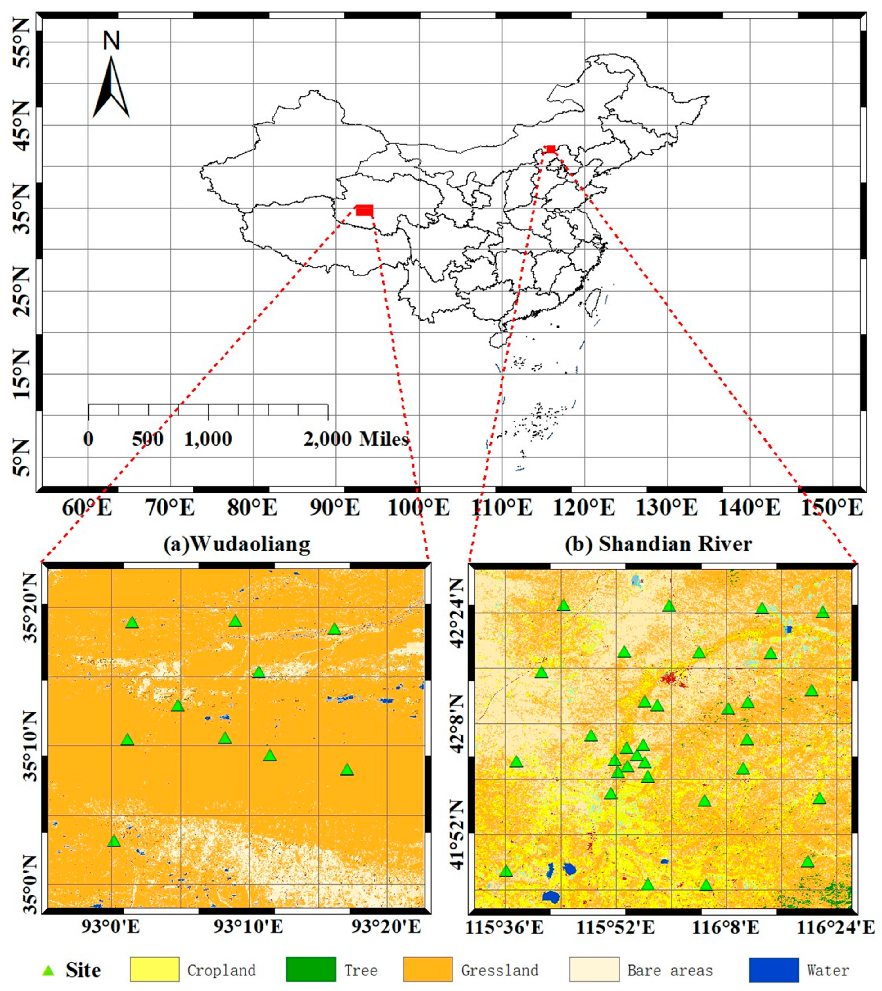
Figure 2.
Flowchart for data processing and soil moisture downscaling.
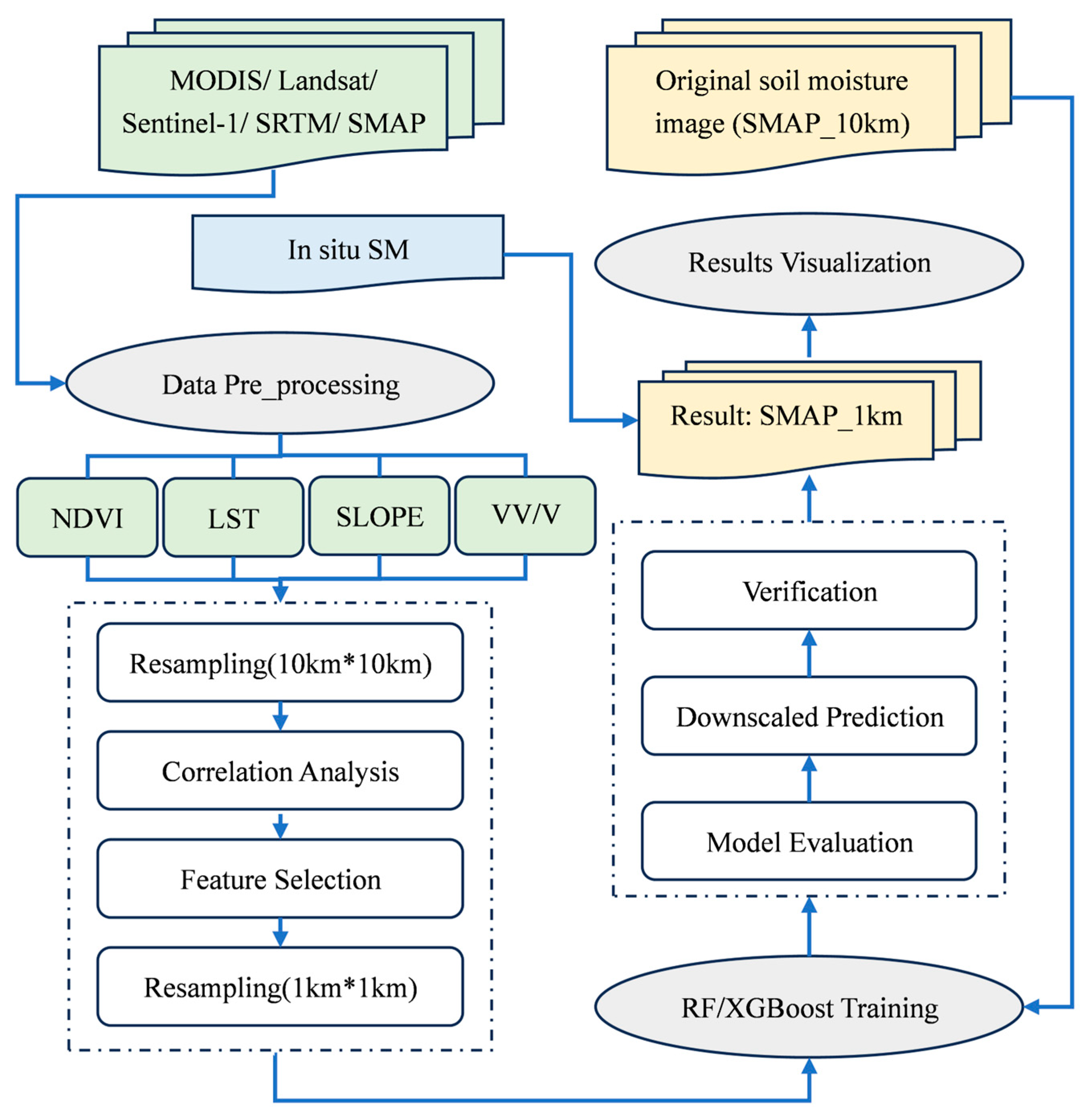
Figure 3.
Heatmap of the R for the model data used for downscaling.
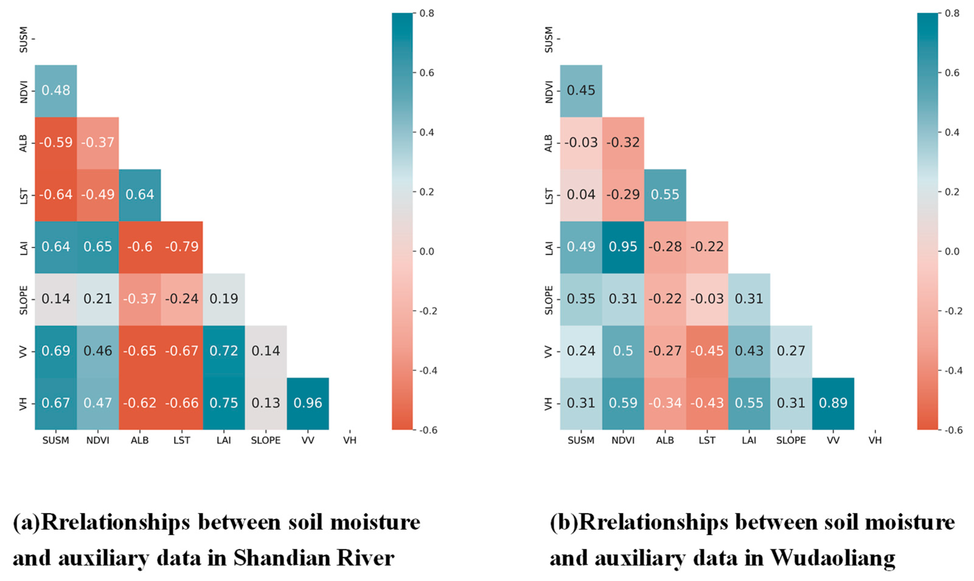
Figure 4.
Various feature weights of the RF.
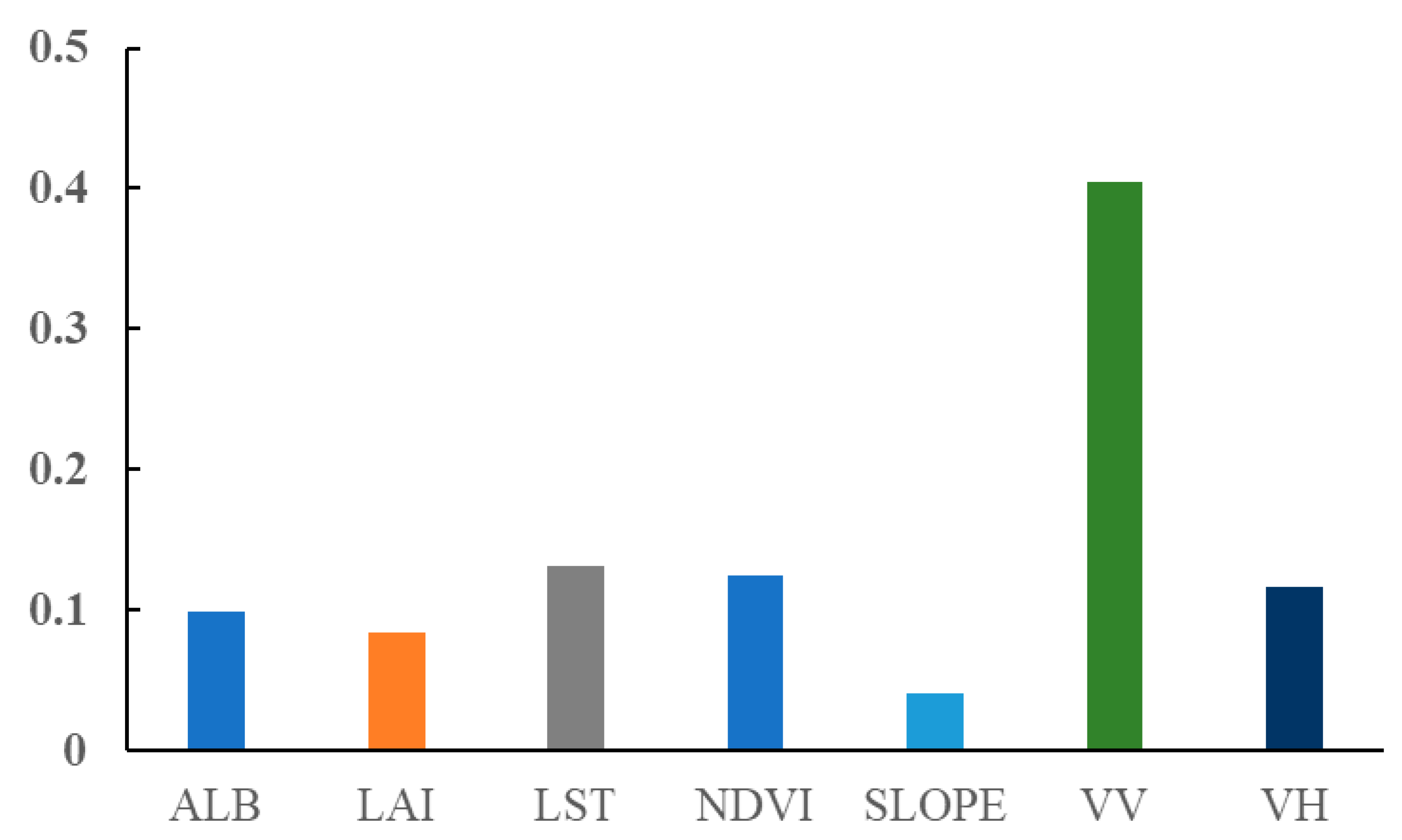
Figure 5.
Soil moisture distributions in the Shandian River Basin before and after downscaling (SMAP_10km is the original soil moisture, SMAP_NOVV_1km is the downscaled soil moisture without SAR backscattering coefficients data, SMAP_1km and SMAP_100m are downscaled soil moisture with adding SAR backscattering coefficients data. The same meaning as below.).
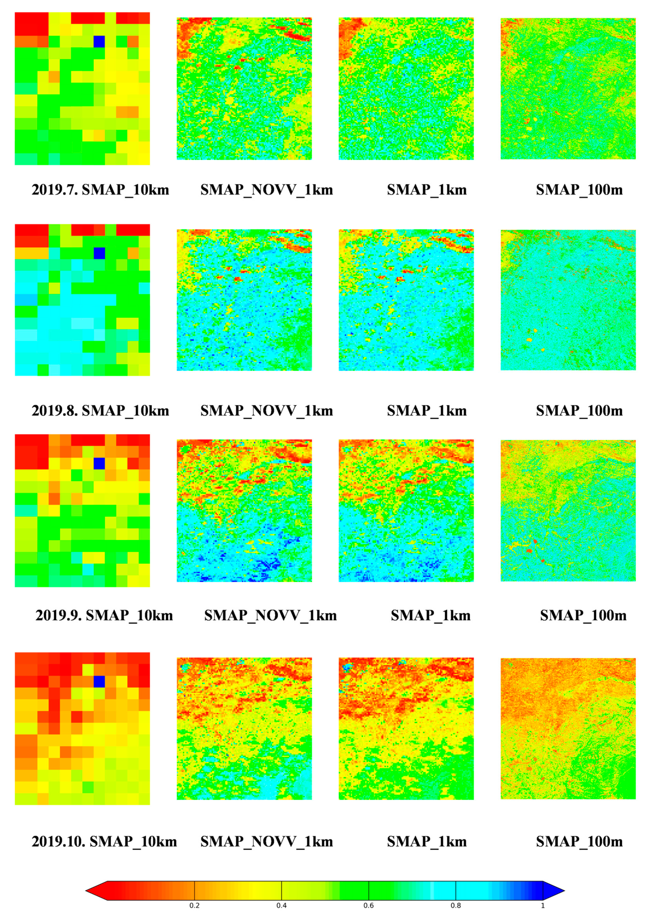
Figure 6.
Soil moisture distributions in the Shandian River Basin before and after downscaling.
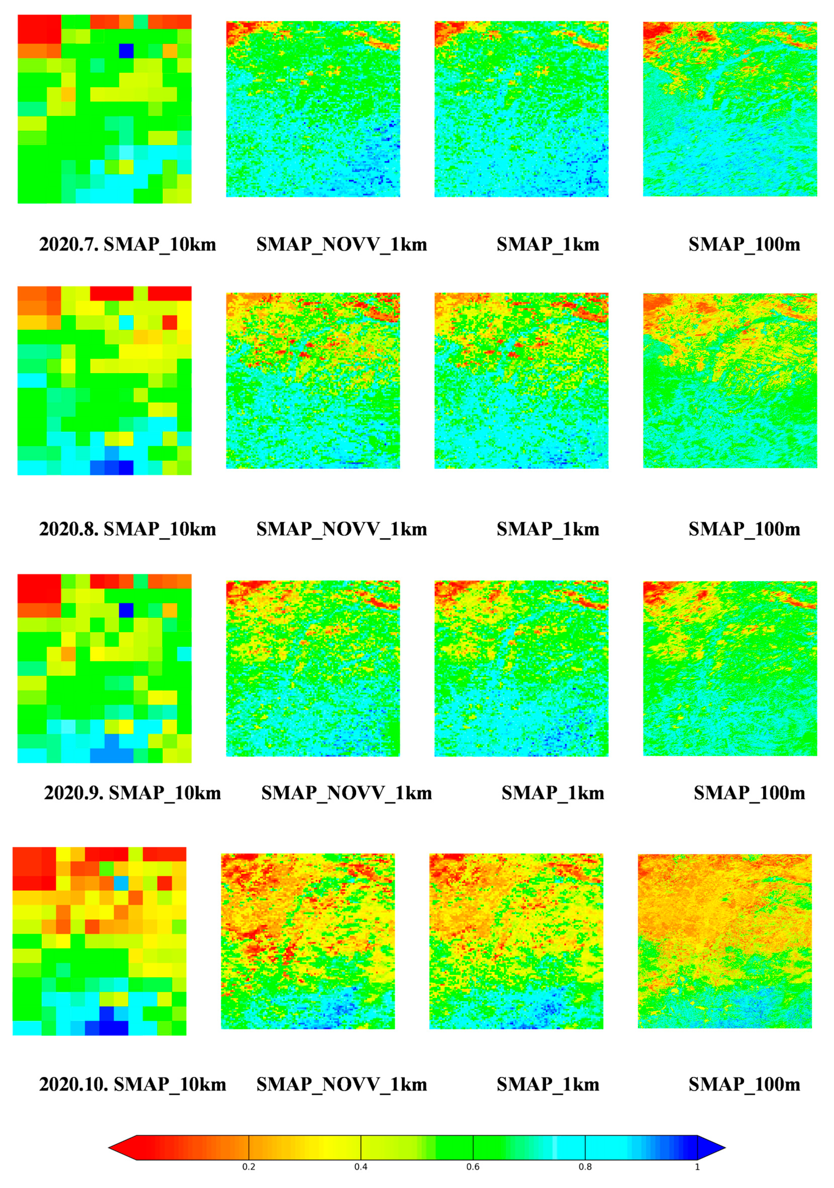
Figure 7.
Soil moisture distributions before and after downscaling in the Wudaoliang area.
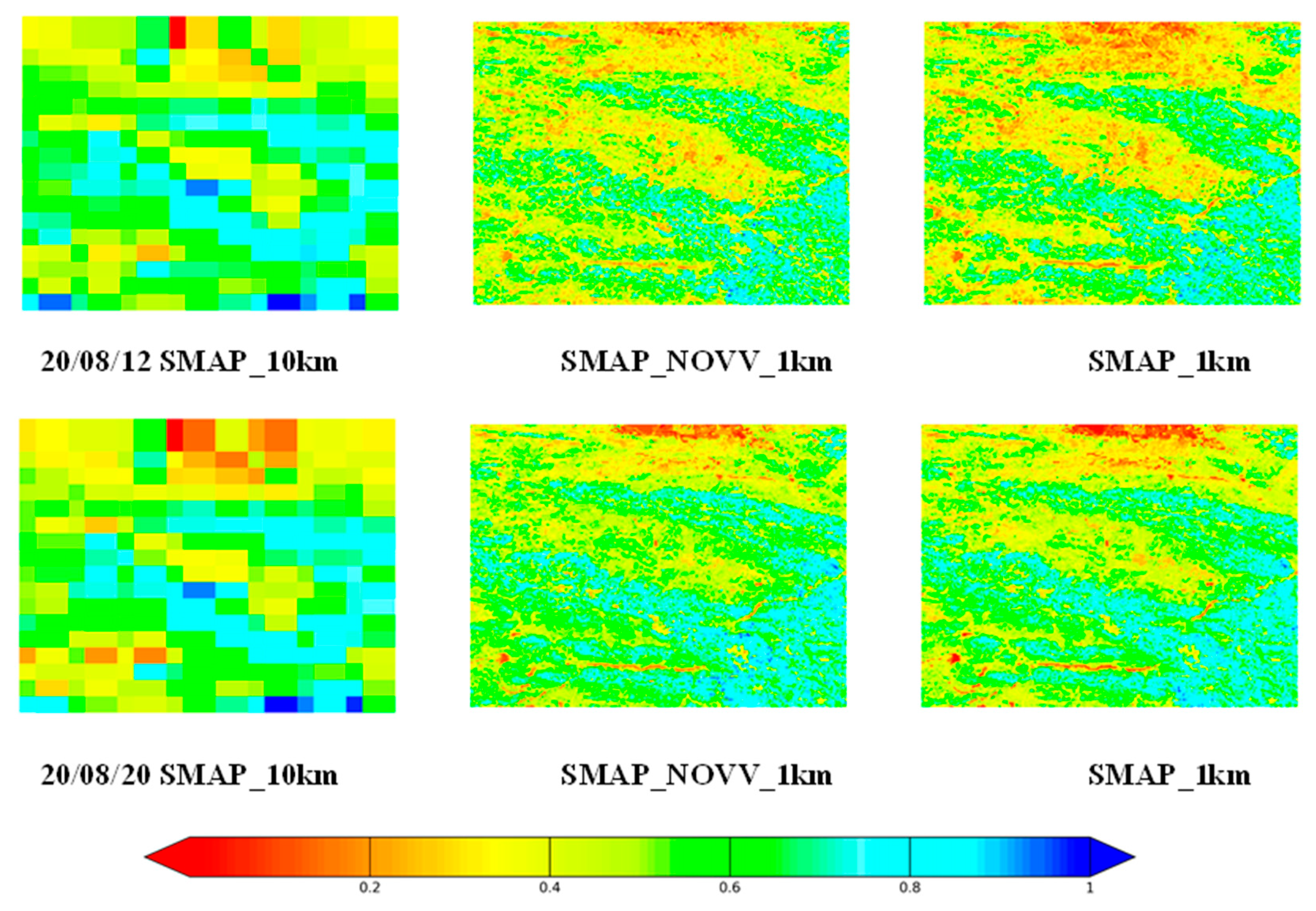
Figure 8.
Scatter plot of before and after downscaling in the Shandian River Basin.
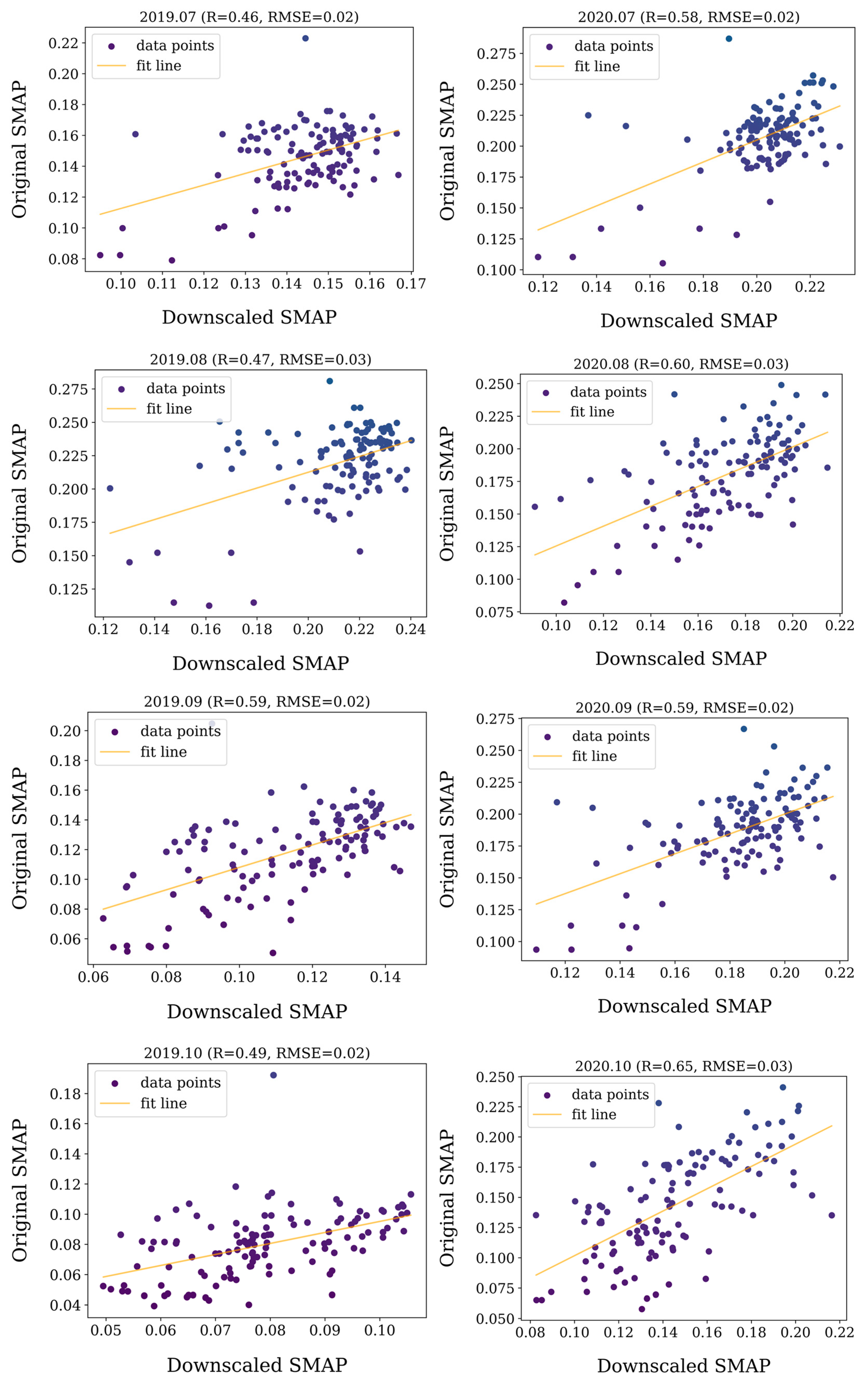
Figure 9.
Comparison of Taylor diagrams before and after downscaling in the Wudaoliang area.
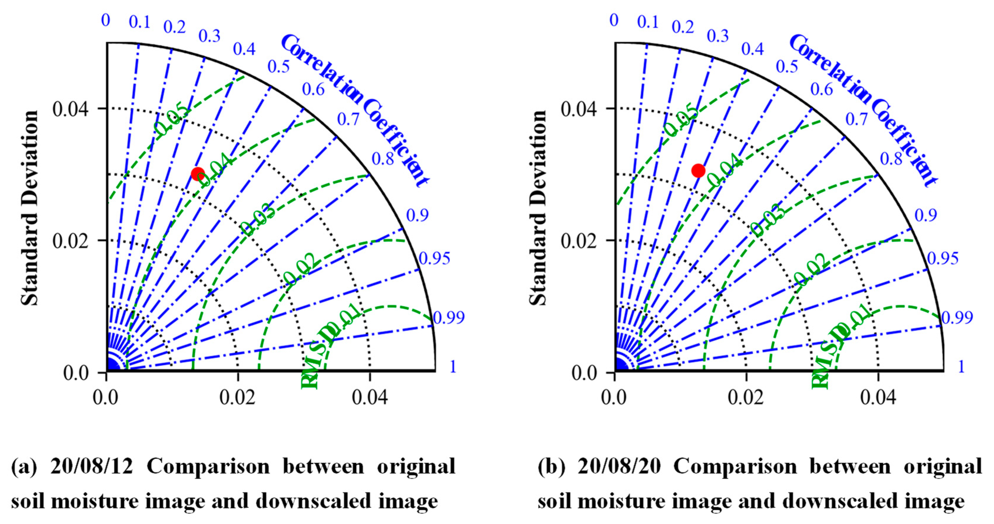
Figure 10.
Scatter plots of downscaled soil moisture and In-situ SM.
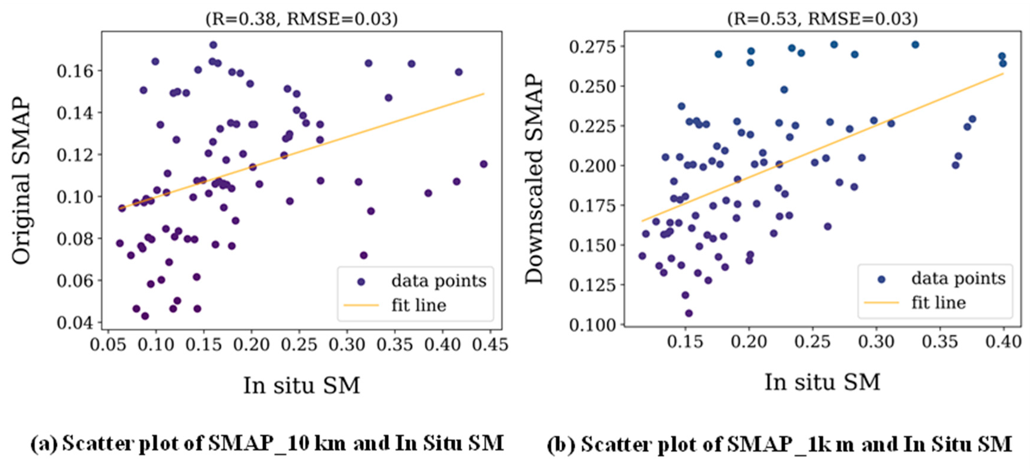
Table 1.
Data.
| Dataset | abbreviation | Spatial resolution/m | Time resolution/day | Aggregation |
|---|---|---|---|---|
| SPL4SMGP MODIS/061/MCD43A3 MODIS/061/MOD15A2H MODIS/061/MCD12Q1 MODIS/061/MOD11A1 MODIS/061/MOD13A2 COPERNICUS/S1_GRD COPERNICUS/S1_GRD CGIAR/SRTM90_V4 LANDSAT/LC08/C02/T1_L2 |
SMAP ALB LAI LC LST NDVI VV VH SLOPE NDVI/LST |
10000 500 500 500 1000 1000 10 10 90 100 |
1 1 1 365 8 16 12 12 15 |
mean mean max mean mean max mean mean mean max/mean |
| Periods | 2019.7-2019.10/2020.7-2020.10 | |||
Table 2.
Model parameter setting details.
| RF | XGB | ||
|---|---|---|---|
| Parameter name | Parameter range | Parameter name | Parameter range |
| n_estimators max_features max_depth min_samples_split min_samples_leaf bootstrap |
[5,20,30,60,80,100] [‘auto’, ‘sqrt’] [10,20,30 ...120] [2,6,12] [1.3,4] [True, False] |
learning_rate n_estimators reg_alpha reg_lambda max_depth min_child_weight seed |
[0.2,0.3] [20,50,60] [0.1,10,20] [0.1,1,10] [2,3] [1,2,4,6] [17,27] |
Table 3.
Comparison of the maximum and mean values of the image before and after downscaling.
| Min(cm3/cm3) | Max(cm3/cm3) | Mean(cm3/cm3) | |
|---|---|---|---|
| Before downscaling | 0.120 | 0.313 | 0.245 |
| After downscaling | 0.137 | 0.300 | 0.227 |
Table 4.
Correlations between remote sensing images and in situ observation (R).
| SDR In-situ SM | WDL In-situ SM | ||
|---|---|---|---|
| 2019 | 2020 | 2020 | |
| 7 8 9 10 | 7 8 9 10 | 08.12 08.20 | |
| SMAP_10km | 0.17 0.20 0.38 -0.13 | 0.26 0.15 0.29 0.22 | -0.6 -0.57 |
| SMAP_NOVV_1km | 0.38 0.27 0.32 -0.12 | 0.24 0.27 0.42 0.38 | 0.46 0.61 |
| SMAP_1km | 0.59 0.42 0.45 0.24 | 0.18 0.35 0.48 0.41 | 0.64 0.75 |
| SMAP_100m | 0.44 0.45 0.53 0.28 | 0.54 0.39 0.27 0.33 |
Disclaimer/Publisher’s Note: The statements, opinions and data contained in all publications are solely those of the individual author(s) and contributor(s) and not of MDPI and/or the editor(s). MDPI and/or the editor(s) disclaim responsibility for any injury to people or property resulting from any ideas, methods, instructions or products referred to in the content. |
© 2024 by the authors. Licensee MDPI, Basel, Switzerland. This article is an open access article distributed under the terms and conditions of the Creative Commons Attribution (CC BY) license (http://creativecommons.org/licenses/by/4.0/).
Copyright: This open access article is published under a Creative Commons CC BY 4.0 license, which permit the free download, distribution, and reuse, provided that the author and preprint are cited in any reuse.


