
Submitted:
21 November 2024
Posted:
25 November 2024
You are already at the latest version
Abstract
This study presents a detailed analysis of various machine learning models for predicting the interfacial bond strength of fiber-reinforced polymer (FRP) concrete, utilizing multiple linear regression, an ensemble of regression trees, Gaussian Process Regression (GPR), Support Vector Regression (SVR), Multigene Genetic Programming (MGGP), and neural network models. The models were evaluated based on their accuracy. The optimal model identified was the GPR ARD model, which achieved a mean absolute error (MAE) of 1.8953 MPa and a correlation coefficient (R) of 0.9658. Analysis of this optimal model highlighted that the three most influential variables affecting the bond strength are the length of the FRP strip (Lf), the thickness of the strip ( tf), and the compressive strength of the concrete to which the strip is applied (fc'). Additionally, the research identified several models with lower expression complexity and reduced accuracy, which may still be applicable in practical scenarios.
Keywords:
Fiber-reinforced polymer
; Bond strength
; Machine learning models
1. Introduction
Fiber-Reinforced Polymers (FRPs) are essential in modern construction due to their high strength-to-weight ratio, corrosion resistance, and ease of application, making them ideal for retrofitting concrete and masonry structures. Retrofitting unreinforced masonry (URM) buildings in earthquake-prone regions with FRPs effectively improves seismic resistance, enhances load-bearing capacity, and increases ductility, addressing vulnerabilities caused by outdated construction techniques [1,2].
Traditional empirical models for predicting FRP-concrete bond strength have shown limitations in accurately capturing the complex interactions between these materials. This has led to a growing interest in applying machine learning (ML) techniques, which are capable of handling large datasets and uncovering intricate patterns that might be missed by conventional approaches. Recent studies have demonstrated the effectiveness of machine learning algorithms.
Wu and Jiang's research (2013) focused on quantifying and modeling interfacial bond parameters through both experimental and analytical studies. They developed a comprehensive database comprising 628 shear tests of externally bonded FRP joints. Their analysis identified key factors affecting bond parameters, particularly focusing on the bond strength and fracture energy. Additionally, they derived new models for the width factor as a function of width ratio and concrete strength, offering more accurate bond strength and fracture energy predictions. This work contributed to understanding how bond behavior is influenced by variables such as the width of the FRP and the strength of the concrete [3].
Zhou et al. (2020) developed an artificial neural network (ANN) model to predict the interfacial bond strength between FRP and concrete. Utilizing a substantial database of 969 test results, they trained the ANN model using backpropagation neural networks (BPNN), incorporating weighted values, biases, and transfer functions. Their model demonstrated higher accuracy than 20 existing models, with significantly lower predictive errors. The study also provided an explicit formula derived from the ANN model, which can be used in practical design applications for predicting bond strength [4].
In their research, Li et al. (2020) compiled a large dataset to assess the bond strength and bond stress-slip behavior of FRP-reinforced concrete members. Their study also incorporated an evaluation of environmental durability factors that could affect bond performance. The study is crucial for its contribution to understanding how reduction factors in bond strength are influenced by both the environment and material properties [5].
Su et al. (2021) explored the potential of machine learning approaches, including multiple linear regression, support vector machine (SVM), and artificial neural networks (ANN), for predicting the interfacial bond strength (IBS) between FRP and concrete. Two datasets were used: Dataset 1 (122 IBS values), and Dataset 2 (136 IBS values). The variables in Dataset 1 include FRP properties such as elastic modulus, tensile strength, and bond length, while Dataset 2 uses fewer input features but focuses on stiffness and groove dimensions. Among the machine learning models, the SVM model demonstrated superior predictive ability with R² values of 0.79 for Dataset 1 and 0.85 for Dataset 2. This research highlights the capability of advanced machine learning models in predicting FRP-concrete bond strength [6].
The study by Haddad and Haddad (2021) employed an artificial neural network (ANN) technique to predict the bond strength between FRP and concrete. The researchers compiled an extensive dataset comprising over 440 data points, allowing the ANN model to assess various parameters such as FRP properties, concrete compressive strength, and bond length. The model demonstrated impressive predictive accuracy, achieving high correlation coefficients (R² nearing 0.98), and significantly outperformed traditional empirical methods. This study underscores the effectiveness of ANN models in predicting complex interactions between FRP and concrete in structural applications [7].
Chen et al. (2021) developed a prediction model using the ensemble learning method known as Gradient Boosted Regression Trees (GBRT) to estimate the interfacial bond strength between FRP and concrete. Their model was trained using a comprehensive database of 520 tested samples. The GBRT model demonstrated superior accuracy, with R² values of 0.9627 during training and 0.9269 during testing. The model outperformed both ANN and SVM models, making it a robust tool for predicting FRP-concrete bond strength in practical engineering applications [8].
Barkhordari et al. (2022) introduced hybrid models that combine population-based algorithms (Bald Eagle Search, Manta Ray Foraging Optimization, and Runge-Kutta optimizer) with ANNs to estimate FRP-concrete interfacial bond strength. The study utilized a dataset of 969 experimental samples and found that the RUN-ANN model achieved the best performance, with an R² value of 0.92. Moreover, the Shapley Additive exPlanations (SHAP) method was used to interpret the model, identifying FRP bond length and width as key factors influencing bond strength predictions [9].
Alabdullh et al. (2022) applied a hybrid ensemble machine learning approach to predict the bond strength of FRP laminates bonded to concrete. Using a database of 136 samples, the team trained and validated several standalone machine learning models, including ANN, Extreme Learning Machine, and GPR. The hybrid ensemble model (HENS) achieved superior predictive accuracy, with an R² value of 0.9783 for training and 0.9287 for testing, demonstrating its effectiveness in overcoming overfitting issues common in traditional machine learning models [10].
In their study, Kim et al. (2022) employed ensemble machine learning techniques to predict FRP-concrete interfacial bond strength. Using a dataset of 855 single-lap shear tests, they evaluated various ensemble methods, with the CatBoost algorithm achieving the best performance. The algorithm showed a root mean square error of 2.310, a covariance of 21.8%, and an R² value of 96.1%, suggesting its high accuracy and potential for practical applications [11].
This research aims to advance existing methodologies by developing a robust machine learning model specifically designed to predict FRP-concrete bond strength, utilizing a comprehensive dataset of experimental results. The study evaluates several machine learning models to identify the most significant input variables and further interprets their predictions using advanced methods for feature importance analysis. Through this approach, the study aims to contribute to the ongoing efforts in optimizing FRP applications in civil engineering, ensuring more reliable and efficient reinforcement solutions.
2. Materials and Methods
2.1. Multiple Linear Regression
Linear regression analysis is a statistical method used to determine the causal effect of one or more independent variables on a dependent variable. When the problem involves one dependent variable () and multiple independent variables (), multiple linear regression can be used. The model can be described by the equation (1):
In this equation is the intercept, are the coefficients of the independent variables, represents the error term.
To estimate the parameters (, ) of the linear model, it is used the least squares method. The goal is to minimize the sum of the squares of the differences between the observed values and the values predicted by the model. This is done using the following equation (2):
where is the vector of estimated parameters, is the matrix of input variables, and is the vector of observed output values.
2.2. Regression Trees Ensembles: Boosted Trees, Bagging and Random Forest
Regression trees are a subset of decision trees tailored to predict continuous outcomes. These models partition the input space into regions using binary recursive splitting, where each leaf represents a specific numerical prediction (Figure 1).
The objective at each node is to select the best split by minimizing the residual sum of squares between the predicted and actual values in the resulting regions [12,13,14].
For a given dataset containing N observations with p input variables, denoted as , where represents an input vector and the corresponding output, the tree construction aims to minimize the following expression (3):
where and are the two regions after splitting on the j-th variable at point s, and are the mean predictions within these regions.
Once the input space is divided into M regions, the prediction for any new observation is the mean of the outcomes for the region to which belongs, given by (4):
where represents the average output in region and is an indicator function that is 1 if and 0 otherwise.
Regression trees, while interpretable and flexible, tend to suffer from high variance, meaning that even small changes in the training data can result in significant differences in the structure and predictions of the tree. This instability makes regression trees prone to overfitting, especially when the model becomes too complex by learning specific noise in the training data.
2.2.1. Boosting Methodology
Boosting is an ensemble learning technique in which models are trained sequentially. Each successive model aims to improve the performance of the ensemble by correcting errors from previous iterations (Figure 2). Specifically, Gradient Boosting focuses on minimizing a predefined loss function by iteratively adding new models to an ensemble [12,13,14]. Each newly added regression tree optimizes its predictions based on the residuals, the differences between the actual and predicted values of the preceding models.
Mathematically, for a given set of training data , where represents the input features and are the target variable, the objective of Gradient Boosting is to minimize a differentiable loss function where is the predicted output. The general form of the model can be expressed as (5):
where represents the final model prediction, is the weight of each weak learner, and is the prediction from the m-th weak learner, typically a regression tree.
At each iteration mmm, the new tree is trained to minimize the residuals from the previous iteration. The residuals at the m-th step are calculated as (6):
In the case of quadratic error (i.e., squared loss), the residuals simplify to (7):
Here, is the predicted value from the ensemble up to iteration m-1. The new regression tree is then fitted to the residuals in order to minimize the overall loss.
2.2.2. Bagging and Random Forest (RF) Methodology
To address limitation of individual regression trees and improve the predictive performance, ensemble methods such as bagging and RF are commonly used (Figure 3). These methods combine multiple decision trees to reduce variance and create more robust models. Bagging (Bootstrap Aggregating) works by generating multiple bootstrap samples from the original dataset. Each sample is created by randomly selecting data points with replacement, meaning some data points may be repeated while others are left out. For each bootstrap sample, a separate regression tree is trained independently. Instead of relying on a single tree, bagging reduces variance by averaging the predictions from all trees in the ensemble, thus providing a more stable and accurate prediction [15,16,17,18,19].
Mathematically, if represents the prediction from the b-th bootstrap sample, the final prediction from bagging is given by the average of all individual predictions (8):
where B is the total number of bootstrap samples, and is the prediction from the b-th regression tree. By averaging the predictions, bagging significantly reduces the model's variance, making it less sensitive to the idiosyncrasies of individual training datasets. This leads to improved generalization on unseen data, while still maintaining the flexibility and interpretability of individual decision trees.
RF build upon bagging by introducing an additional layer of randomness. Instead of considering all variables for each split, RF select a random subset of the variables at each node, which decorrelates the trees and further reduces variance. This process ensures that no single variable dominates the tree-building process.
2.3. Support Vector Regression (SVR)
Support Vector Regression (SVR) is an adaptation of the Support Vector Machines (SVM) algorithm, designed for continuous output prediction tasks. SVR transforms the input space into a higher-dimensional feature space using kernel functions, allowing for the linear separation of data points that may not be linearly separable in the original input space [20,21,22].
Given a dataset where and are the corresponding continuous output values, the goal of SVR is to find a function that has at most an deviation from the actual output for all training data while maintaining a balance between model complexity and prediction error. The regression function in SVR is given by (9):
where is a non-linear transformation of the input into a higher-dimensional space, is the weight vector, and b is the bias term. This model aims to minimize the following objective (10):
where is the regularization term that controls the model complexity, is a regularization parameter that determines the trade-off between the model’s complexity and its tolerance to deviations, and is the loss function with an -insensitive zone, defined as (11):
This loss function ensures that deviations within are ignored, focusing only on larger errors.
Minimizing is equivalent to minimizing (12):
where and are the slack variables, which are shown in Figure 4.
The optimization problem in SVR is typically solved using Lagrange multipliers, transforming the problem into its dual form. The dual form allows the incorporation of kernel functions, which can compute inner products in the high-dimensional feature space without explicitly mapping the input vectors to that space. This is crucial for handling non-linear relationships within the data.
The dual optimization problem can be expressed as (13):
subject to the constraints (14):
where and are Lagrange multipliers, is the kernel function that computes the dot product in the feature space without explicitly performing the transformation. The kernel function can take various forms which facilitate the mapping of input data into higher-dimensional spaces suitable for separation.
The prediction function for new data points in SVR is then given by (15):
Commonly used kernel functions in SVR include:
- Linear kernel
- Sigmoid kernel:
- Radial Basis Function (RBF) kernel .
The performance of the SVR model depends heavily on selecting appropriate hyper parameters, such as: regularization parameter C, ϵ, kernel-specific parameters, where for instance, γ in the RBF kernel, which controls the width of the Gaussian function etc. Tuning these hyper parameters is crucial for ensuring the model generalizes well to unseen data. This is typically achieved using grid search techniques to identify the optimal values for C, ϵ, and any kernel-specific parameters.
2.4. Gaussian Process Regression (GPR)
Gaussian Process Regression (GPR) is a Bayesian regression technique that offers a probabilistic framework for modeling the relationship between input features and continuous output variables. One of the significant advantages of GPR is its ability to quantify uncertainty in predictions [23].
In GPR, it is assumed that the underlying function mapping inputs to outputs is sampled from a Gaussian Process. A Gaussian Process is characterized as a collection of random variables where any finite number of these variables have a joint Gaussian distribution.
Consider the nonlinear regression problem (16):
Here, is an unknown function mapping the input to the output , and represents normally distributed noise with mean zero and variance . GPR assumes that the unknown function follows a Gaussian Process, which is specified by a mean function and a covariance function (or kernel)
Given a dataset with observations, , these observations are modeled as a sample from a multivariate Gaussian distribution (17):
where:
is the vector of mean values.
K is the covariance matrix, where the element , with being the Kronecker delta function.
For a new test input , GPR predicts its corresponding output . The joint distribution of both the training data outputs and the new output is a multivariate Gaussian distribution (18):
where:
- is the mean vector.
- is the covariance matrix, which can be divided into blocks (19):
In this matrix:
- is the covariance between the test point and training points.
- is the variance at the test point.
The conditional distribution of given the training data is also Gaussian, with mean and variance values, respectively (20), (21):
The covariance function (kernel) plays a key role in defining the properties of the functions that the GP can model. A commonly used kernel is the Squared Exponential (SE) kernel with Automatic Relevance Determination (ARD) (22):
In this equation controls the length scale for each input dimension, indicating how much influence each dimension has on the prediction. A large means the corresponding input dimension is less important.
The parameters and the noise variance are called hyper parameters. These can be optimized by maximizing the log marginal likelihood of the observed data (23):
2.5. Multi Gene Genetic Programming
Genetic Programming (GP) is an evolutionary algorithm-based methodology used for modeling and optimization. It generates models by simulating the process of natural selection, where a population of potential solutions evolves over time, with the best solutions "surviving" and "reproducing." This methodology is particularly suited to problems where the functional form of the model is not known beforehand.
In regression tasks, GP evolves models that predict continuous outputs based on input variables. The objective is to find a symbolic representation (a mathematical formula) that best approximates the relationship between input and output data. The flexibility of GP allows it to discover complex, non-linear relationships that may be difficult to capture using traditional regression techniques [24,25].
The process starts by generating an initial population of random solutions (Figure 5). Each individual in this population represents a possible model for the problem and it is structured using one or more decision trees. In the initial iteration, the tree model is generated by randomly selecting mathematical functions, constants, and model variables. Within this framework, each tree can be thought of as representing a single "gene" in the model. The trees culminate in terminal nodes, which are assigned either as input variables from the model or as fixed constants. All other intermediate nodes in the tree serve as functional nodes.
Each model in the population is evaluated based on a fitness function, which quantifies how well the model performs in predicting the desired output. Commonly used metrics include the Root Mean Square Error (RMSE), Mean Absolute Error (MAE), and other error-based criteria.
Selection process of models is based on their fitness and models with better performance have a higher probability of being selected, but some randomness is introduced to maintain diversity within the population.
Selected models are paired to create new "offspring" models by exchanging parts of their structures (Figure 6). In constructing new models, the best-performing models from the previous generation are utilized to generate a new population through processes such as crossover, mutation, and direct copying. In practice, the selection of models for reproduction is probabilistic, based on their fitness score or the complexity of the model structure. Model complexity is often determined by the number of nodes and subtrees within a tree, reflecting the expressive capacity of the model.
During the crossover process, genetic material from two parent models can be exchanged entirely or partially (Figure 6). For example, suppose the model contains the genes and another model contains the genes . If we select a random set of genes for crossover, the models may look like (24), (25):
The bolded genes represent those selected for crossover, and their exchange results in the following offspring (26), (27):
This high-level crossover process enables the creation of new models that inherit features from both parent models.
Additionally, crossover can occur at the gene level, known as low-level crossover, where only a portion of a gene is exchanged.
In such cases, only part of the tree is altered (as seen in Figures 6a and 6b). Mutation can also occur at this level, where a node within a gene is randomly selected, and a newly created subtree is inserted at that location (Figures 6c and 6d). These evolutionary procedures are repeated over multiple generations to refine the model.
The resulting model is pseudo-linear, as it represents a linear combination of non-linear components modeled as trees. Mathematically, this multigene regression model is represented as [24,25]:
where is the bias term, are the scaling parameters, and are the outputs from the i-th tree (gene).
The overall gene response matrix is denoted by:
with dimensionality , and the coefficient vector is:
The vector b is estimated using the least-squares method, and its solution is computed as:
Thus, the final multigene regression model can be written as:
The process of selection, crossover, and mutation is repeated over many generations. Over time, the population evolves, and the models typically improve in performance. The algorithm terminates when a stopping criterion is met. This criterion could be a pre-defined number of generations, reaching a certain fitness threshold, or convergence in the population.
2.6. Artificial Neural Networks
A Multi-Layer Perceptron (MLP) is a type of feedforward neural network designed for supervised learning tasks (Figure 7). Its architecture consists of an input layer, one or more hidden layers, and an output layer. Each layer is composed of neurons that receive signals, process them through weighted synaptic connections, and apply a non-linear activation function to generate an output [14,26].
The input layer receives the data, which is then propagated through the network. Each neuron in the hidden layers processes the inputs by computing a weighted sum of its inputs, adding a bias term, and applying a non-linear activation function such as the hyperbolic tangent function. The output layer neurons typically use a linear activation function when the model is applied to regression tasks.
Mathematically, the activation of a neuron a hidden layer can be expressed as (33):
where are the input variables, represent the weights for neuron , is the bias term, and ϕ is the activation function.
The number of neurons in the hidden layers is a critical parameter in MLP design. The selection of this number can influence the model’s performance and its ability to generalize to unseen data. The number of neurons is typically determined through experimental tuning, following various heuristic guidelines that relate the number of neurons to the dimensions of the input and output data.
The maximum number of neurons was selected as the upper limit, and various network architectures were explored, beginning with a single neuron in the hidden layer. Subsequent architectures incrementally increased the number of neurons up to the maximum value determined by the following equation (34) [12]:
The choice of activation function plays a pivotal role in the learning capacity of the MLP. In this model, a hyperbolic tangent (tanh) activation function is employed in the hidden layer neurons. For the output layer, a linear activation function is utilized, which is suitable for regression problems.
The MLP model can be trained using LM algorithm, where weights are updated iteratively through gradient descent. The loss function, the mean squared error (MSE), is minimized during training to improve the accuracy of the model.
3. Dataset
The database consists of 855 test results collected from 38 research studies (Table 1), focusing on the key parameters that influence bond strength [2]. The single-lap shear test (Figure 8), recognized as one of the most effective methods for evaluating the bond strength at the FRP-concrete interface, forms the foundation of this study.
The collected dataset includes critical material properties and geometric parameters. Material properties encompass the compressive strength of a concrete cylinder (), and the elastic modulus of FRP sheets. Geometric parameters include the thickness () and width () of the FRP sheet, the bond length () of the FRP sheet, and the width of the concrete substrate (). The compressive strength of concrete cubes samples () was converted to cylinder strength ().
The filtered dataset was divided into a training set (70% of the data) for model development and a test set (30% of the data) for assessing model performance. Depending on the model, MSE (Mean Squared Error) or RMSE (Root Mean Squared Error) was used as the primary metric during training. Model accuracy on the test set was evaluated using four metrics: two absolute measures (RMSE and MAE) and two relative measures (MAPE and the correlation coefficient R). This process is illustrated in Figure 9.
The Mean Squared Error (MSE) is calculated using (35):
where:
- actual value (target),
- predicted value,
N – total number of training samples.
The Root Mean Squared Error (RMSE) is a measure of overall model accuracy, expressed in the same units as the predicted variable (36):
RMSE is sensitive to larger errors due to the squaring process, making it effective for identifying significant prediction discrepancies.
The Mean Absolute Error (MAE) measures the average absolute difference between predicted and actual values (37):
Unlike RMSE, MAE gives equal importance to all errors, regardless of their size.
The Mean Absolute Percentage Error (MAPE), sometimes referred to as the Mean Absolute Percentage Deviation (MAPD), is a metric for assessing prediction accuracy and is calculated as follows (38):
In this formula (38), the absolute difference between each observed value () and predicted value () is divided by the observed value. This ratio is summed for all samples, averaged by dividing by the total number of samples, and finally multiplied by 100. MAPE is not suitable if any observed values are zero.
The Pearson correlation coefficient (R) is used as a relative measure to evaluate the relationship between observed and predicted values (39):
where:
- average of predicted values,
- average of actual values.
The division of the complete dataset for machine learning models should be conducted in a manner that ensures similar statistical characteristics across subsets. This approach aims to create training, validation, and test sets with comparable distributions and statistical indicators, such as mean, standard deviation, and data range, thereby preserving data integrity and enhancing the model's ability to generalize effectively (Table 2, Table 3).
The following flowchart presents a step-by-step procedure for building a machine learning model to predict the output variable (kN). Each model is evaluated to determine the one that best meets the desired accuracy, making it a candidate for potential deployment.
4. Results and Discussion
A linear regression framework, enhanced not only with main effects but also with various interaction and polynomial terms, was employed to capture the complexities in bond strength prediction.
Interaction terms, such as , etc. allow us to examine how pairs of variables jointly influence bond strength, capturing multi-variable dependencies essential when one variable’s effect is modified by another.
Polynomial terms (squares of the variables), like , , etc. addressed nonlinear relationships between predictors and bond strength, enabling the model to fit complex trends while retaining the interpretability of linear regression.
By broadening the model to include these interaction and polynomial terms, we achieved improved predictive accuracy, as validated by RMSE, MAE, MAPE, and R metrics.
The Table 4. presents the estimated coefficients, standard errors, t-statistics, and p-values for each parameter in the developed linear regression model. The most significant predictors of bond strength are the interaction between FRP thickness and sheet width (), the interaction between FRP elastic modulus and thickness (), FRP elastic modulus (), and concrete compressive strength (), along with their interactions.
Polynomial terms indicate that the relationship between certain variables and bond strength is not strictly linear, with diminishing effects observed at higher values.
Performance metrics including Root Mean Squared Error (RMSE), Mean Absolute Error (MAE), Mean Absolute Percentage Error (MAPE), and the correlation coefficient (R) were calculated to assess the model's (defined by equation (40)) accuracy.
The obtained regression equation is defined by the following expression (40):
In this research, a Gradient Boosted Trees (GBT) ensemble was employed, with a grid search approach used to systematically explore and optimize the model’s key parameters. The grid search was applied to various combinations of learning rates and tree complexities to identify the best-performing configuration. Following values were investigated:
- Number of Generated Trees (NumLearningCycles = 100): The ensemble was limited to 100 trees to balance model complexity and prevent overfitting. This parameter was kept constant during the grid search to evaluate the impact of the learning rate and tree depth more precisely.
- Learning Rate (λ): Grid search was used to explore learning rates ranging from 0.001 to 1.0. The search revealed that a learning rate of 0.1 provided the best trade-off between fast convergence and error minimization.
- Number of Splits (MaxNumSplits): Tree depth, represented by the maximum number of splits, was also varied in the grid search. The search evaluated depths ranging from 1 split (shallow trees) to 512 splits (deep trees). Tree complexity was controlled by adjusting the maximum number of splits (MaxNumSplits), calculated in relation to dataset size. The maximum depth of the trees was determined using the formula , where n is the number of data points and rounded to a whole number. The term n - 1 is used because the number of possible splits equals n - 1, which considers the total number of internal nodes required to split between adjacent points. Taking the logarithm of n−1 for base 2 helps determine the approximate number of splits required for full separation of the dataset. This value is then rounded to the nearest whole number to represent the maximum depth of the decision tree in terms of the number of splits. This depth calculation ensures that the trees are not too deep relative to the dataset size, which helps prevent overfitting.
The grid search identified the combination of 64 splits and a learning rate of 0.25 as the best, achieving the lowest RMSE of 3.3427 and the highest R value of 0.9536. The best MAE of 2.2542 was achieved with 128 splits and a learning rate of 0.1. The lowest MAPE was observed with 64 splits and a learning rate of 0.1, yielding a value of 0.1503 (Figure 10).
The optimal number of splits can be adopted to be 64, where the model achieved its best performance across several metrics. Beyond 64 splits, further increases in tree depth yielded diminishing returns, as seen by the leveling off of improvements in RMSE and R-squared value. Learning curve for optimal model is represented with purple color in Figure 11.
In this study, permutation error was employed to determine the relative importance of each input variable in the GBT model developed to predict the output variable . The permutation importance method quantifies variable significance by assessing the increase in prediction error when the values of each variable are randomly shuffled, thereby disrupting its relationship with the target variable. This technique is particularly advantageous for understanding the contribution of each predictor in complex, nonlinear models like gradient boosting. The results, illustrated in Figure 12, reveal that variables (width of the FRP) and (bond length) have the highest importance, significantly influencing the model's accuracy. In contrast, variables such as (concrete width) and (concrete compressive strength) have a lesser impact on the predictive power.
Bagging (Bootstrap Aggregation) is the primary method used to implement the ensemble model in this research. Depending on whether we use only a subset of the input variables or the entire set of variables, a RF or TreeBagger model will be created, respectively. This method involves creating multiple decision trees (500 trees in your case) on different bootstrap samples of the data and averaging their predictions to improve model robustness and reduce variance.
The research specified 500 learning cycles (NumLearningCycles = 500), meaning 500 base decision trees are trained, and their predictions are aggregated to form the final output. This large number of trees stabilizes the model and helps capture complex patterns in the data.
Two hyper parameters are tuned during the training process: Min Leaf Size and Number of Variables to Sample at each split.
- Min Leaf Size: This parameter controls the minimum number of observations required to form a leaf in a decision tree. Smaller leaf sizes result in deeper trees, allowing the model to capture more detailed patterns in the data but also increasing the risk of overfitting. In this implementation, Min Leaf Size is varied from 1 to 10.
- Number of Variables to Sample: At each split in a decision tree, a subset of predictor variables is randomly selected for consideration. The number of variables sampled at each split (NumVariablesToSample) is varied from 1 to 6.
Across all metrics (RMSE, MAE, MAPE, and R), smaller Min Leaf Size values (especially 1 and 2) consistently lead to better results (Figure 13). This suggests that deeper trees, which allow for more detailed splits, are necessary to capture the complexity in the data. The best-performing models used 3 or 4 variables for splitting at each node. This aligns with the idea that a moderate number of variables strikes a balance between simplicity and model complexity.
The best configurations identified are:
- Best RMSE: 3.7860, with Min Leaf Size = 1 and Number of Variables = 3.
- Best MAE: 2.5821, with Min Leaf Size = 1 and Number of Variables = 4.
- Best MAPE: 0.1778, with Min Leaf Size = 1 and Number of Variables = 4.
- Best R-squared: 0.9415, with Min Leaf Size = 1 and Number of Variables = 3.
There is consistency in the best-performing configurations across the different evaluation metrics (RMSE, MAE, MAPE, and R). The model with Min Leaf Size = 1 and Number of Variables = 3 or 4 appears to be a robust choice for optimal performance across various metrics.
The SVR used a radial basis function (RBF), linear and sigmoid kernel and applied grid search cross-validation to optimize the hyper parameters of the SVR model. All data were normalized. Normalization scales the data to a range between 0 and 1 by subtracting the minimum value and dividing by the range (max-min). This step is critical in SVR because the optimization process is sensitive to the scale of the input data. After normalization, the training and testing data were used in the SVR model.
Grid search is used to find the optimal values for three SVR hyper parameters:
- C (cost/regularization): This controls the trade-off between allowing slack variables (errors) and forcing the decision boundary to be as tight as possible. A higher C makes the model focus more on correctly classifying all training points but risks overfitting.
- Gamma (γ): This defines the influence of individual training examples. Smaller values of gamma imply that each training point has a far-reaching influence, while higher values imply more localized influence.
- Epsilon (ε): This defines a margin of tolerance where no penalty is given to errors within a certain range. Epsilon controls the sensitivity of the model to prediction errors.
First, the analysis of the application of the RBF kernel was performed. The parameters , , and are varied from -5 to 5 in coarse increments of 1. For each combination of C, , and , an SVR model is trained, and the MSE is calculated on the test set. The best combination of hyper parameters is identified by minimizing the MSE.
Finer grid search is applied around the best values of C, gamma, and epsilon found in the coarse grid search. The step size is reduced to half the previous value, and a smaller search range is applied around the best initial values. The model is iteratively again retrained for each combination, and MSE is recalculated to find the refined best parameters. The accuracy criterion values for the analyzed models are given in Table 5.
An analogous procedure was applied to the other two kernel functions. The optimal models were determined with following kernel parameters:
- C = 1.4513; ε = 0.0043; γ = 20.7363 for the RBF kernel;
- C = 0.3208 and ε = 0.0432 for the linear kernel;
- C = 23.6326; ε = 0.0521; γ = 0.0118 for sigmoid kernel.
In this research, various covariance functions were employed to design the GPR model, each with different strengths in modeling the relationships between the input variables and the target. The covariance functions explored included the exponential, squared exponential, Matérn (with 3/2 and 5/2 degrees of smoothness), and rational quadratic kernels. These kernels control how the model captures correlations in the data, effectively shaping how predictions are influenced by nearby points. Additionally, Automatic Relevance Determination (ARD) versions of these kernels were tested, which assign individual length scales to each input variable. This feature allows the model to automatically determine the relative importance of each predictor, improving performance in datasets with features of varying significance.
To ensure comparability between features and prevent any single feature from disproportionately affecting the model, the input data was standardized. The standardization was achieved using Z-score normalization, where each feature is rescaled to have a mean of zero and a standard deviation of one.
This transformation is essential in GPR models to ensure that all variables contribute appropriately to the prediction process, especially when using covariance functions sensitive to the scale of the input data.
The GPR model employed a constant basis function, meaning the model assumes a fixed baseline for the predictions, allowing the kernel functions to capture the complexity in the relationships. The model was trained and evaluated using a holdout validation approach.
The parameters of the covariance functions used in the analysis were optimized through gradient-based methods, applied to the log marginal likelihood expression (Table 6, Table 7)). The length scale values for each input variable offer insights into the importance of these variables concerning the model’s predictive performance (Table 7). Variables with smaller length scales tend to have a greater influence on the model, as the relationship between the input and output changes more rapidly with those features. In contrast, larger length scales indicate less significant features.
All models with ARD perform better than their non-ARD counterparts (Table 8, Table 9). The ARD mechanism allows the models to focus on the most important features, leading to better predictive performance and lower error metrics.
The provided Figure 14 uses the inverse of these length scales to visually highlight variable importance, the smaller the length scale, the larger the corresponding bar in the graph, indicating greater influence on the output. The results indicate that among all the input variables, the bond length of FRP () plays the most crucial role in predicting bond strength. This could be due to the strong relationship between the bond area and the bond strength. The thickness of FRP () and concrete compressive strength () are also important but to a lesser extent, aligning with structural engineering principles where material properties impact bonding but not as strongly as the bond length. The relatively low importance of and suggests that variations in these factors do not significantly alter the model’s predictions for bond strength, potentially because their influence is overshadowed by the more dominant variables.
In this study, it is implemented a Multigene Genetic Programming (MGGP) approach that involved a comprehensive analysis of different values for the number of genes and varying tree depths, both of which are critical parameters that determine the complexity and performance of the resulting models. The method aimed to explore a wide range of configurations to identify the optimal balance between model complexity and predictive accuracy.
The MGGP method was designed to iteratively search through the solution space by repeating the procedure ten times in this research. This iterative repetition was necessary to address the inherent randomness in the initialization of model parameters. Each iteration began with a random set of parameters, resulting in a unique model at the end of each run.
The parameter settings used in this study are summarized in Table 10, which provides key details such as the function set, population size, number of generations, maximum number of genes, and maximum tree depth. These parameters were carefully chosen to enable an extensive exploration of possible model structures while maintaining control over computational complexity. Specifically, models were analyzed with the number of genes ranging from one to six and tree depths varying from one to six. These settings allowed the study to capture a wide range of model structures, from simple to highly complex.
During the training process, two main objectives were prioritized: minimizing RMSE and minimizing the expression complexity of the models. These two factors were treated as part of a multi-objective function, balancing prediction accuracy with interpretability. RMSE was used as a standard measure with weight of 0.7 of model accuracy, indicating how well the model predictions aligned with the actual data. Meanwhile, expression complexity with weight of 0.3 was an important metric for ensuring that the resulting models remained interpretable, avoiding overly complex expressions that would be difficult to understand or deploy.
To enhance the robustness of the results, the process was repeated over 1000 generations, allowing the evolutionary process to refine the models over time. The population size initially was set to 100, ensuring that a diverse range of solutions could be explored in each generation. After all number of generations is achieved process is restarted and repeated and new models are created. These multiple models, derived from ten independent runs, were ultimately merged to form one final population that was representative of the most promising solutions.
These models were then subjected to a detailed evaluation, focusing on their correlation coefficients and expression complexities. The models that exhibited superior correlation coefficients, indicating strong predictive power, and lower complexity were selected for further analysis. This selection formed what is known as the Pareto front (as depicted in Figure 11). The Pareto front represents the set of models that provide the best possible trade-offs between competing objectives namely, accuracy and complexity. By selecting models along this front, we ensured that the final set of models included those that were both effective in making accurate predictions and interpretable due to their reduced complexity.
The use of a tournament selection mechanism, with a size of 2, allowed for a balance between exploration and exploitation of the solution space. The elitism rate of 0.05% ensured that the best individuals from each generation were preserved, preventing the loss of high-quality solutions. Crossover and mutation probabilities were set to 0.84 and 0.14, respectively, to encourage diversity within the population and prevent premature convergence.
The MGGP approach used in this study involved an extensive analysis of different model configurations, focusing on balancing accuracy and complexity. By iteratively generating and evaluating models, and ultimately selecting those along the Pareto front, we were able to identify models that were both accurate and interpretable (Figure 15). This approach ensured that the final model was not only effective in terms of predictive performance but also practical for real-world applications due to its manageable complexity.
The analytical expression of the optimal Pareto front model (Model ID 7961) is defined by the following equation (41):
Analytical expressions for individual genes are given in the Table 11.
Each of the symbolic analytical expressions or genes listed in the Table 11 is also structurally represented in the form of a tree in Figure 16.
The relationship between the accuracy of the obtained model which consists of a population of 800 individuals and two parameters, namely the Number of Genes and the Depth of the Tree, is illustrated in the Figure 17. The Pareto front depicted in the Figure 15 is defined using two criteria: the values RMSE and the coefficient of determination R². It represents a set of non-inferior (Pareto-optimal) solutions based on these criteria. The GPTIPS software used for model creation in this research highlights the optimal model according to RMSE and R² criteria with a green circle outlined in red. Since the analysis in this study was conducted using the criteria of RMSE, MAE, MAPE, and Correlation Coefficient R, each model from the aforementioned set of non-inferior solutions was further analyzed concerning all defined criteria. This was done to identify a potential model with lower complexity.
From the Table 12, it can be observed that the optimal model from the set of non-inferior solutions, with a complexity of 95, has very similar accuracy to the model labeled as Model ID 6959, which has a complexity of 42. Regarding the three defined criteria MAE, MAPE, and R, the differences are almost negligible, while in terms of RMSE, the difference appears in the first decimal place.
By applying this lower-complexity model, a mathematical expression significantly simpler for practical use is obtained, whose accuracy is only slightly less than that of the optimal model.
By employing the MGGP model using the GPTIPS software [22 ,65}, models were developed where only variables significant to the problem which is researched were retained through evolutionary processes.
Throughout this evolutionary process, variables that do not significantly contribute to the model's accuracy are generally eliminated, resulting in a final model comprising only the most relevant predictors. However, in this particular analysis, all six input variables were found to contribute to the model's accuracy and thus need to be incorporated into the model formulation.
The analytical expression of the model (Model 6959) with reduced complexity is defined by the following equation (42):
Analytical expressions for individual genes for Model 6959 (MGGP simplified) are given in Table 13.
The neural network model architecture was established through a trial-and-error method. In this study, the input layer comprises 6 neurons, and the output layer consists of a single neuron.
The optimal number of neurons in the hidden layer was determined experimentally. Beginning with a single neuron, the number of neurons was incrementally increased, with each configuration assessed based on RMSE, MAE, R, and MAPE metrics. Models utilizing the Levenberg-Marquardt (LM) algorithm were tested, with data divided into same training and test sets for analysis.
All model variables underwent linear transformation to ensure all variables were scaled to the range [−1,1]. Here, the minimum value was mapped to -1 and the maximum to 1, with intermediate values scaled linearly. Scaling was applied to equalize the influence of each variable, as a variable’s absolute size may not reflect its actual impact. The same standard settings in MATLAB were applied across all model architectures during training (Table 14).
As guidelines for estimating the upper limit of the neuron count in the hidden layer, the previously mentioned expressions were used, with a recommendation to adopt the lower value as follows:
The RMSE, MAE, MAPE, and R values for different network architectures, tested with up to 23 neurons, are illustrated in the Figure 18.
These metrics indicate that the model with 13 neurons in the hidden layer achieved optimal performance, close to the upper boundary of the initially tested range. Consequently, the range was expanded to evaluate the impact of additional neurons. However, adding more neurons did not enhance accuracy; rather, it highlighted a risk of overfitting. Beyond this limit, the model began to fit too closely to the training data, reducing its ability to generalize effectively to unseen data.
A comparative analysis of all analyzed models according to the adopted accuracy criteria is given in the Table 15.
Table 15 presents a comparative analysis of several machine learning models used for predicting bond strength, evaluated based on four key accuracy metrics: Root Mean Squared Error (RMSE), Mean Absolute Error (MAE), Mean Absolute Percentage Error (MAPE), and the correlation coefficient (R). Among the models evaluated, the GPR ARD Exponential model outperforms all others, with the lowest RMSE (2.8671 MPa), MAE (1.9319 MPa), and MAPE (0.1329%) while achieving the highest correlation coefficient (R = 0.9658). This indicates its superior accuracy and predictive power.
The Gradient Boosted model also shows strong performance, with an RMSE of 3.3427 MPa and an R of 0.9536, making it a competitive alternative for situations requiring complex, non-linear modeling. Similarly, RF and TreeBagger models also perform well, with RMSE values of 3.7860 MPa and 3.8302 MPa, respectively, and R values above 0.939. These models are effective in reducing variance and offer robustness through ensemble learning.
The SVR RBF model, while slightly less accurate than the tree-based models, still achieves reasonable results with an R of 0.9332 and a relatively low MAE (3.5352 MPa), suggesting its applicability in scenarios where a simpler model is preferred.
On the other hand, the MGGP and MGGP simplified models, despite their interpretability, show lower accuracy with higher RMSE values (4.4436 MPa and 4.6829 MPa, respectively). This indicates that while these models may be useful for applications requiring simple, symbolic expressions, they may not be the best choice when high accuracy is critical.
Finally, the Neural Network (NN 6-13-1) model, with an RMSE of 4.0992 MPa and R of 0.9293, offers a balanced trade-off between model complexity and accuracy. However, it still falls short compared to the top-performing models like GPR and Gradient Boosted.
In summary, the GPR ARD Exponential model is the optimal choice based on all evaluated metrics, though simpler models such as Gradient Boosted or RF may still be valuable depending on the application, especially in terms of balancing complexity and performance.
Figure 19 shows a regression plot, comparing the target values with the predicted values from the model. This plot illustrates the accuracy of the model's predictions, with the closer the predicted values are to the target values, the better the model's performance. The regression plot reflects a strong correlation between the actual and predicted results, indicating the model's ability to effectively capture the relationship between the input features and bond strength.
Figure 20 provides a direct comparison between the target and predicted values for the optimal GPR ARD Exponential model. This visual further demonstrates how well the model predicts the bond strength, with the predictions closely matching the target values across the dataset. The closeness of the predicted values to the target values confirms the high accuracy and reliability of the model in predicting bond strength.
While the model is relatively complex, a MATLAB Graphical User Interface (GUI) was developed to facilitate practical implementation by experts. The model's code includes a built-in database, making it easy to adapt the model through the expansion of the database with additional data. The MATLAB code is provided in the Appendix A1. The GUI functions by allowing the user to input the corresponding values for the six input variables, and the prediction is obtained by clicking the 'Predict Bond Strength' button (Figure 21).
5. Conclusions
In this research, a comprehensive evaluation of machine learning models was conducted to predict the interfacial bond strength of fiber-reinforced polymer (FRP) applied to concrete. Using an extensive dataset of 855 experimental results from 38 studies, the study assessed multiple advanced algorithms, including multiple linear regression with interactions, ensemble methods (Gradient Boosted Trees, TreeBagger, Random Forest), Support Vector Regression (SVR), Gaussian Process Regression (GPR), Multigene Genetic Programming (MGGP), and neural networks.
Among the models evaluated, GPR with Automatic Relevance Determination (ARD) proved to be the most accurate, achieving an RMSE of 2.8671 MPa, MAE od 1.8953 MPa and a correlation coefficient (R) of 0.9658. This model identified the FRP bond length, FRP thickness, and concrete compressive strength as the most significant predictors of bond strength, emphasizing their roles in effective FRP-concrete reinforcement.
The Gradient Boosted Trees ensemble model also showed high accuracy with an RMSE of 3.3427 MPa, MAE of 2.2603 MPa and R of 0.9536, especially when optimized through grid search for learning rate and tree depth, making it a strong candidate for complex, non-linear interactions between variables. While MGGP achieved slightly lower accuracy, it provided interpretable models that balance predictive performance with simplicity, which is advantageous for practical applications.
This analysis demonstrated that the choice of machine learning model impacts predictive accuracy, with ensemble methods and GPR offering robust, high-performing options for predicting FRP-concrete bond strength.
Additionally, by leveraging interaction terms and polynomial features for linear regression, the study enhanced the models' ability to capture the non-linear relationships inherent to FRP-concrete interactions, resulting in a direct and straightforward expression that is practically applicable.
This research underscores the potential of machine learning to enhance the reliability of FRP applications in structural engineering, contributing valuable insights to civil engineering reinforcement techniques.
Supplementary Materials
The supplementary materials accompanying the article include a detailed MATLAB model for implementing the optimal Gaussian Process Regression with Automatic Relevance Determination (GPR ARD) model. This package is complemented by a user-friendly graphical user interface (GUI) that allows users to interactively explore the model’s capabilities, adjust parameters, and visualize the results. The MATLAB model and GUI for the optimal GPR ARD model are available online at https://www.mdpi.com/article/.
Author Contributions
Conceptualization, M.K., M.H-N and P.P.; methodology, M.K, M.H-N and P.P.; software, M.K., M.H-N and P.P; validation, M.K., T.V. and M.R.; formal analysis, M.K., T.V. and M.R.; investigation, M.K.; resources, M.H-N.; data curation, M.K., T.V. and M.R.; writing—original draft preparation, M.K. and M.H.-N; writing—review and editing, M.K., M.H-N and P.P.; visualization, M.K., T.V. and M.R.; supervision, M.H-N.; project administration, M.H-N.; funding acquisition, M.H-N.; All authors have read and agreed to the published version of the manuscript.
Funding
This research received no external funding
Data Availability Statement
All experimental data used for developing the GPR ARD model is included in the MATLAB file for creating the model and the corresponding graphical user interface. In addition, the training and test datasets, as well as the entire database, are provided in the form of an attached Excel file.
Conflicts of Interest
The authors declare no conflicts of interest.
References
- Hadzima-Nyarko, M.; Čolak, S.; Bulajić, B.Đ.; Ademović, N. Assessment of Selected Models for FRP-Retrofitted URM Walls under In-Plane Loads. Buildings 2021, 11, 559. [CrossRef]
- Hadzima-Nyarko, M.; Ademović, N.; Pavić, G.; Kalman Šipoš, T. Strengthening techniques for masonry structures of cultural heritage according to recent Croatian provisions. Earthquakes and Structures 2018, 15, 473–485. [CrossRef]
- Wu, Y.; Jiang, C. Quantification of Bond-Slip Relationship for Externally Bonded FRP-to-Concrete Joints. J. Compos. Constr. 2013, 17, 673–686. [CrossRef]
- Zhou, Y.; Zheng, S.; Huang, Z.; Sui, L.; Chen, Y. Explicit Neural Network Model for Predicting FRP-Concrete Interfacial Bond Strength Based on a Large Database. Compos. Struct. 2020, 240, 111998. [CrossRef]
- Li, J.; Gravina, R. J.; Smith, S. T.; Visintin, P. Bond Strength and Bond Stress-Slip Analysis of FRP Bar to Concrete Incorporating Environmental Durability. Constr. Build. Mater. 2020, 261, 119860. [CrossRef]
- Su, M.; Zhong, Q.; Peng, H.; Li, S. Selected Machine Learning Approaches for Predicting the Interfacial Bond Strength between FRPs and Concrete. Constr. Build. Mater. 2021, 270, 121456. [CrossRef]
- Haddad, R.; Haddad, M. Predicting FRP-concrete bond strength using artificial neural networks: A comparative analysis study. Struct. Concr. 2021, 22, 38-49.
- Chen, S.-Z.; Zhang, S.-Y.; Han, W.-S.; Wu, G. Ensemble Learning Based Approach for FRP-Concrete Bond Strength Prediction. Constr. Build. Mater. 2021, 302, 124230. [CrossRef]
- Barkhordari, M.S.; Armaghani, D.J.; Sabri, M.M.S.; Ulrikh, D.V.; Ahmad, M. The Efficiency of Hybrid Intelligent Models in Predicting Fiber-Reinforced Polymer Concrete Interfacial-Bond Strength. Materials 2022, 15, 3019. [CrossRef]
- Alabdullh, A.A.; Biswas, R.; Gudainiyan, J.; Khan, K.; Bujbarah, A.H.; Alabdulwahab, Q.A.; Amin, M.N.; Iqbal, M. Hybrid Ensemble Model for Predicting the Strength of FRP Laminates Bonded to the Concrete. Polymers 2022, 14, 3505. [CrossRef]
- Kim, B.; Lee, D.-E.; Hu, G.; Natarajan, Y.; Preethaa, S.; Rathinakumar, A.P. Ensemble Machine Learning-Based Approach for Predicting of FRP–Concrete Interfacial Bonding. Mathematics 2022, 10, 231. [CrossRef]
- Elith, J.; Leathwick, J.R.; Hastie, T. A working guide to boosted regression trees. J. Anim. Ecol., 2008, 77, 802–813. [CrossRef]
- Hastie, T.; Tibsirani, R.; Friedman, J. The Elements of Statistical Learning; Springer: Berlin/Heidelberg, Germany, 2009.
- Kovačević, M.; Ivanišević, N.; Petronijević, P.; Despotović, V. Construction cost estimation of reinforced and prestressed concrete bridges using machine learning. Građevinar, 2021, 73, 1-13. [CrossRef]
- Breiman, L.; Friedman, H.; Olsen, R.; Stone, C.J. Classification and Regression Trees; Chapman and Hall/CRC: Wadsworth, OH, USA, 1984.
- Breiman, L. Bagging predictors. Mach. Learn. 1996, 24, 123–140. [CrossRef]
- Breiman, L. Random forests. Mach. Learn. 2001, 45, 5–32. [CrossRef]
- Freund, Y.; Schapire, R.E. A decision-theoretic generalization of on-line learning and an application to boosting. J. Comput. Syst. Sci., 1997, 55, 119–139. [CrossRef]
- Friedman, J.H. Greedy function approximation: A gradient boosting machine. Ann. Stat. 2001, 29, 1189–1232.
- Vapnik, V. The Nature of Statistical Learning Theory; Springer: New York, NY, USA, 1995.
- Kecman, V. Learning and Soft Computing: Support. In Vector Machines, Neural Networks, and Fuzzy Logic Models; MIT Press: Cambridge, MA, USA, 2001.
- Smola, A.J.; Sholkopf, B. A tutorial on support vector regression. Stat. Comput. 2004, 14, 199–222.
- Rasmussen, C.E.; Williams, C.K. Gaussian Processes for Machine Learning; The MIT Press: Cambridge, MA, USA, 2006.
- Searson, D.P.; Leahy, D. E.; Willis , M.J. GPTIPS: An Open Source Genetic Programming Toolbox For Multigene Symbolic Regression, Proceeding of International MultiConference of Engineers and Computer Scieintist Vol. I, IMECS 2010, March 17 – 19, 2010, Hong Kong.
- Kovačević, M.; Lozančić, S.; Nyarko, E.K.; Hadzima-Nyarko, M. Application of Artificial Intelligence Methods for Predicting the Compressive Strength of Self-Compacting Concrete with Class F Fly Ash. Materials 2022, 15, 4191. [CrossRef]
- Hagan, M.T.; Menhaj, M.B., Training Feedforward Networks with Marquardt Algorithm. IEEE Transactions on Neural Networks,1994, 5(6), 989-993.
- Adhikary, B.; Mutsuyoshi, H. Study on the Bond between Concrete and Externally Bonded CFRP Sheet. In Proceedings of the 5th International Symposium on Fiber Reinforced Concrete Structures (FRPRCS-5); Thomas Telford Publishing: London, 2001; pp. 371–378.
- Bilotta, A.; Di Ludovico, M.; Nigro, E. FRP-to-Concrete Interface Debonding: Experimental Calibration of a Capacity Model. Compos. Part B Eng. 2011, 42, 1539–1553. [CrossRef]
- Bilotta, A.; Ceroni, F.; Di Ludovico, M.; Nigro, E.; Pecce, M.; Manfredi, G. Bond Efficiency of EBR and NSM FRP Systems for Strengthening Concrete Members. J. Compos. Constr. 2011, 15, 629–638. [CrossRef]
- Bimal, B.A.; Hiroshi, M. Study on the Bond Between Concrete and Externally Bonded CFRP Sheet. In Proceedings of the 5th International Symposium on FRP Reinforcement for Concrete Structures; University of Cambridge: Cambridge, 2001; pp. 371–378.
- Pellegrino, C.; Tinazzi, D.; Modena, C. Experimental Study on Bond Behavior Between Concrete and FRP Reinforcement. J. Compos. Constr. 2008, 12, 180–188. [CrossRef]
- Chajes, M.J.; Finch, W.W., Jr.; Januszka, T.F.; Thomson, T.A., Jr. Bond and Force Transfer of Composite-Material Plates Bonded to Concrete. Struct. J. 1996, 93, 209–217. [CrossRef]
- Czaderski, C.; Olia, S. EN-Core Round Robin Testing Program – Contribution of Empa. In Proceedings of the 6th International Conference on FRP Composites in Civil Engineering (CICE 2012); Rome, Italy, June 13–15, 2012; pp. 1–8. Available online: https://www.dora.lib4ri.ch/empa/islandora/object/empa:9237.
- Dai, J.-G.; Sato, Y.; Ueda, T. Improving the load transfer and effective bond length for FRP composites bonded to concrete. Proc. Jpn. Concr. Inst. 2002, 24(1), 1423–1428.
- Faella, C.; Nigro, E.; Martinelli, E.; Sabatino, M.; Salerno, N.; Mantegazza, G. Aderenza tra calcestruzzo e Lamine di FRP utilizzate come placcaggio di elementi inflessi. Parte I: Risultati sperimentali. In Proceedings of the XIV Congresso C.T.E., Mantova, Italy, 2002; pp. 7–8.
- Fen, Z.L.; Gu, X.L.; Zhang, W.P.; Liu, L.M. Experimental study on bond behavior between carbon fiber reinforced polymer and concrete. Structural Engineering 2008, 24(4).
- Hosseini, A.; Mostofinejad, D. Effective Bond Length of FRP-to-Concrete Adhesively-Bonded Joints: Experimental Evaluation of Existing Models. Int. J. Adhes. Adhes. 2014, 48, 150–158. [CrossRef]
- Kanakubo, T.; Nakaba, K.; Yoshida, T.; Yoshizawa, H. A Proposal for the Local Bond Stress–Slip Relationship between Continuous Fiber Sheets and Concrete. Concrete Research and Technology 2001, 12(1), 33–43. [In Japanese. [CrossRef]
- Kamiharako, A.; Shimomura, T.; Maruyama, K. The Influence of the Substrate on the Bond Behavior of Continuous Fiber Sheet. Proc. Jpn. Concr. Inst. 2003, 25(3), 1735–1740.
- Ko, H.; Matthys, S.; Palmieri, A.; Sato, Y. Development of a simplified bond stress–slip model for bonded FRP–concrete interfaces. Construction and Building Materials 2014, 68, 142–157. [CrossRef]
- Liu, J. Effect of Concrete Strength on Interfacial Bond Behavior of CFRP–Concrete; Ph.D. Thesis, Shenzhen University, Shenzhen, China, 2012. [In Chinese.].
- Lu, X.Z.; Ye, L.P.; Teng, J.G.; Jiang, J.J. Meso-Scale Finite Element Model for FRP Sheets/Plates Bonded to Concrete. Engineering Structures 2005, 27(4), 564–575. [CrossRef]
- Maeda, T.; Asano, Y.; Sato, Y.; Ueda, T.; Kakuta, Y. A study on bond mechanism of carbon fiber sheet. Proceedings of the 3rd International Symposium on Non-Metallic (FRP) Reinforcement for Concrete Structures, Japan, 1997; pp. 279–285.
- Nakaba, K.; Kanakubo, T.; Furuta, T.; Yoshizawa, H. Bond behavior between fiber-reinforced polymer laminates and concrete. ACI Struct. J. 2001, 98(3), 359–367.
- Pham, H.B.; Al-Mahaidi, R. Modelling of CFRP–Concrete Shear-Lap Tests. Construction and Building Materials 2007, 21(4), 727–735. [CrossRef]
- Ren, H. Study on Basic Mechanical Properties and Long-Term Mechanical Properties of Concrete Structures Strengthened with Fiber Reinforced Polymer; Ph.D. Thesis, Dalian University of Technology, Dalian, China, 2003. [In Chinese.].
- Savoia, M.; Ferracuti, B. Strengthening of RC Structure by FRP: Experimental Analyses and Numerical Modelling; Ph.D. Thesis, DISTART, University of Bologna, Bologna, Italy, 2006.
- Savoia, M.; Bilotta, A.; Ceroni, F.; Di Ludovico, M.; Fava, G.; Ferracuti, B.; et al. Experimental Round Robin Test on FRP–Concrete Bonding. In Proceedings of the 9th International Symposium on Fiber Reinforced Polymer Reinforcement for Concrete Structures (FRPRCS-9); Sydney, Australia, 13–15 July 2009.
- Sharma, S.K.; Mohamed Ali, M.S.; Goldar, D.; Sikdar, P.K. Plate–Concrete Interfacial Bond Strength of FRP and Metallic Plated Concrete Specimens. Composites Part B: Engineering 2006, 37(1), 54–63. [CrossRef]
- Tan, Z. Experimental Study on the Performance of Concrete Beams Strengthened with GFRP; Master's Thesis, Tsinghua University, Beijing, China, 2002. [In Chinese.].
- Taljsten, B. Plate Bonding: Strengthening of Existing Concrete Structures with Epoxy Bonded Plates of Steel or Fibre Reinforced Plastics; Ph.D. Thesis, Luleå University of Technology, Luleå, Sweden, 1994.
- Takeo, M.; Tanaka, T. Analytical solution for bond-slip behavior in FRP-concrete systems. Compos. Struct. 2020, 240, 111998.
- Toutanji, H.; Saxena, P.; Zhao, L.; Ooi, T. Prediction of Interfacial Bond Failure of FRP–Concrete Surface. J. Compos. Constr. 2007, 11(4), 427–436. [CrossRef]
- Ueda, T.; Sato, Y.; Asano, Y. Experimental Study on Bond Strength of Continuous Carbon Fiber Sheet. In Proceedings of the 4th International Symposium on Fiber Reinforced Polymer Reinforcement for Reinforced Concrete Structures; ACI: Farmington Hills, MI, USA, 1999; pp. 407–416.
- Ueno, S.; Toutanji, H.; Vuddandam, R. Introduction of a Stress State Criterion to Predict Bond Strength between FRP and Concrete Substrate. Journal of Composites for Construction 2015, 19(1), 04014028. [CrossRef]
- Wu, Y.-F.; Jiang, C. Quantification of Bond-Slip Relationship for Externally Bonded FRP-to-Concrete Joints. Journal of Composites for Construction 2013, 17(5), 673–686. [CrossRef]
- Wu, Z.S.; Yuan, H.; Yoshizawa, H.; Kanakubo, T. Experimental/Analytical Study on Interfacial Fracture Energy and Fracture Propagation Along FRP–Concrete Interface. In Fracture Mechanics for Concrete Materials: Testing and Applications; SP-201; American Concrete Institute: Farmington Hills, MI, USA, 2001.
- Woo, H.; Lee, H. Bond strength degradation in FRP-strengthened concrete under cyclic loads. Compos. Struct. 2004, 64, 7–16.
- Fu, Q.; Xu, J.; Jian, G.G.; Yu, C. Bond Strength between CFRP Sheets and Concrete. In FRP Composites in Civil Engineering; Teng, J.G., Ed.; Proceedings of the International Conference on FRP Composites in Civil Engineering (CICE 2001), Hong Kong, China, 12–15 December 2001; Elsevier Science: Oxford, UK, 2001; pp. 357–364.
- Yao, J. Debonding in FRP-Strengthened RC Structures; Ph.D. Thesis, The Hong Kong Polytechnic University, Hong Kong, China, 2004.
- Yuan, H.; Wu, Z.S.; Yoshizawa, H. Theoretical solutions on interfacial stress transfer of externally bonded steel/composite laminates. JSCE 2001, 18, 27–39.
- Zhang, H.; Smith, S.T. Fibre-Reinforced Polymer (FRP)-to-Concrete Joints Anchored with FRP Anchors: Tests and Experimental Trends. Can. J. Civ. Eng. 2013, 40(8), 731–742. [CrossRef]
- Zhao, H.D.; Zhang, Y.; Zhao, M. Study on Bond Behavior of Carbon Fiber Sheet and Concrete Base. In Proceedings of the First Chinese Academic Conference on FRP-Concrete Structures; Building Research Institute of Ministry of Metallurgical Industry: Beijing, China, 2000. [In Chinese.].
- Zhou, Y.W. Analytical and Experimental Study on the Strength and Ductility of FRP–Reinforced High Strength Concrete Beam; Ph.D. Thesis, Dalian University of Technology, Dalian, China. [In Chinese.].
- Searson, D.P. GPTIPS 2: An Open-Source Software Platform for Symbolic Data Mining. In Handbook of Genetic Programming Applications; Gandomi, A.H., Ed.; Springer: New York, NY, USA, 2015; Chapter 22.
Figure 1.
Region-based space partitioning a) and 3D regression surface in a regression tree b).
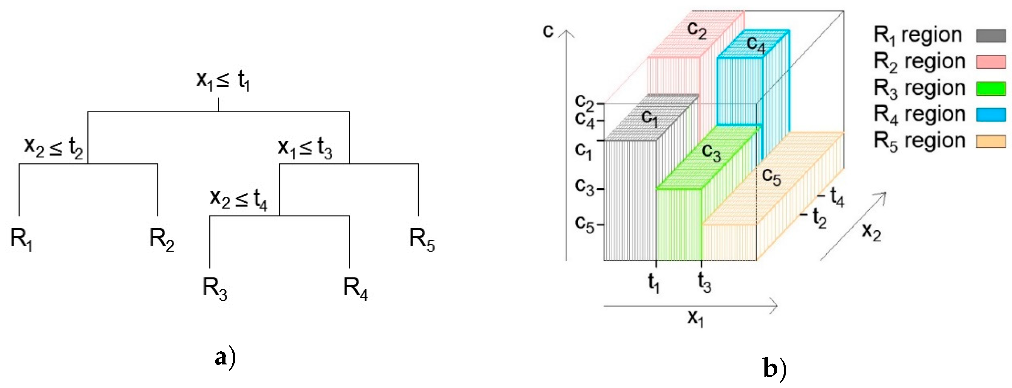
Figure 2.
Gradient boosting ensemble model.
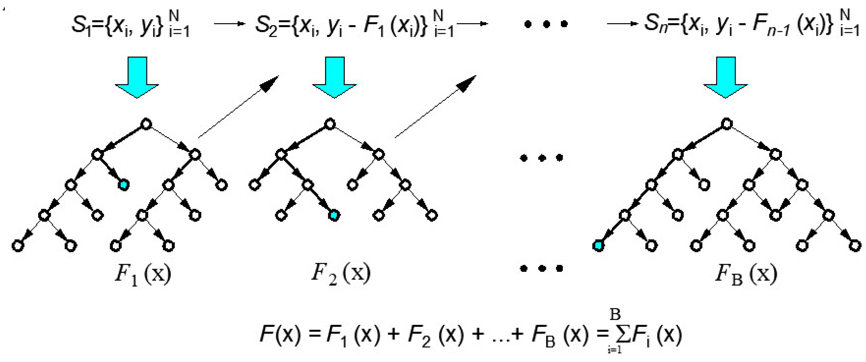
Figure 3.
Bootstrap aggregation (Bagging) in regression tree ensembles.
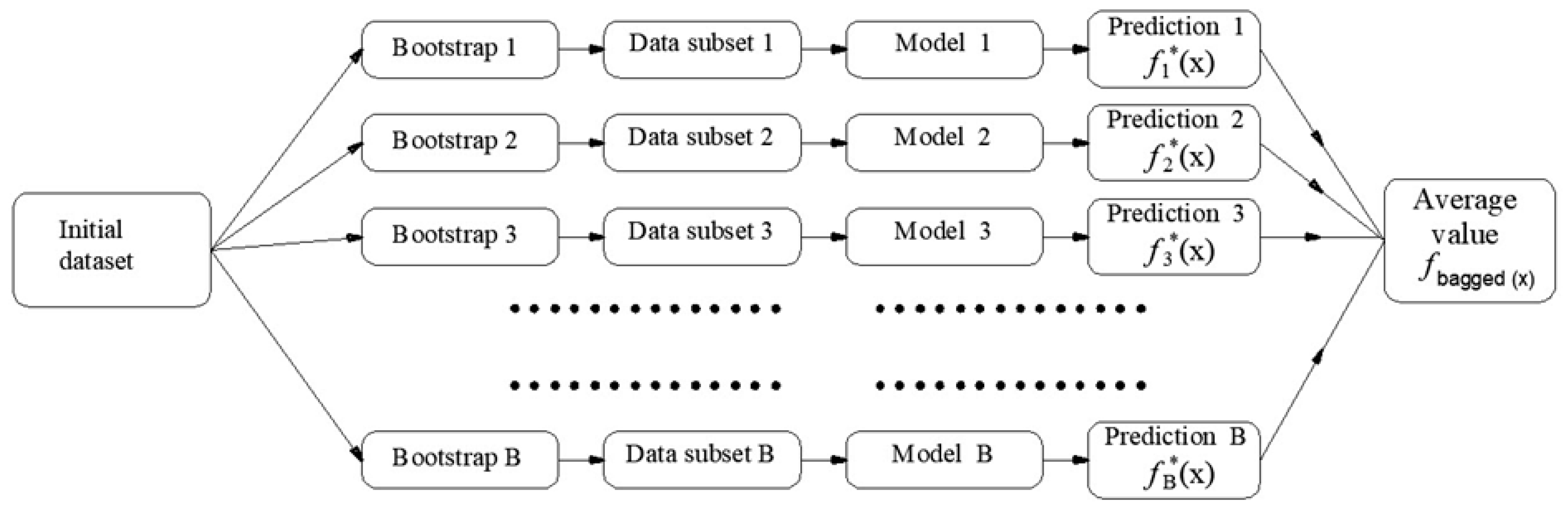
Figure 4.
Nonlinear support vector regression with ε-insensitivity zone [14].
Figure 4.
Nonlinear support vector regression with ε-insensitivity zone [14].
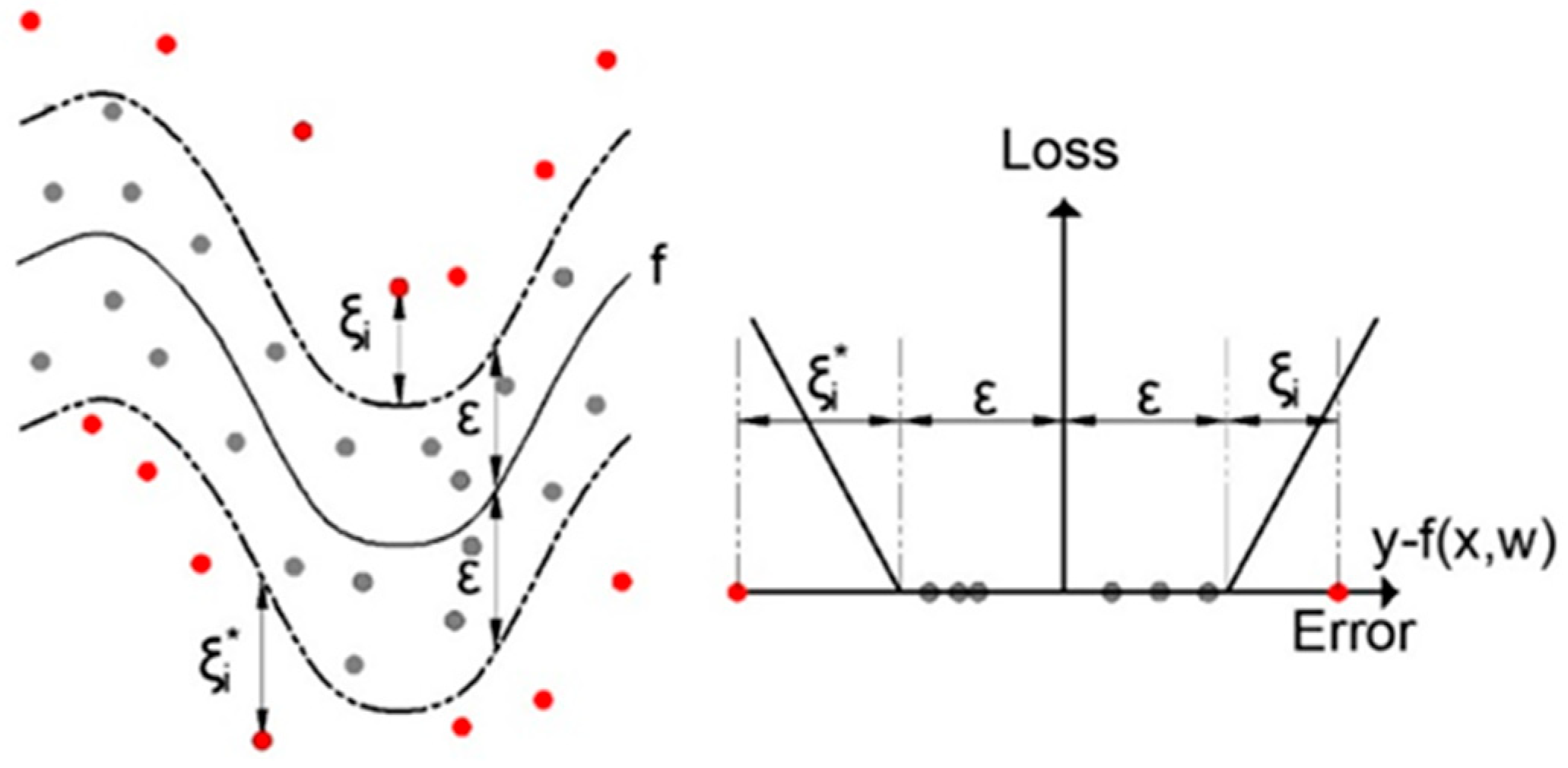
Figure 5.
Example of an MGGP model with two genes [25].
Figure 5.
Example of an MGGP model with two genes [25].
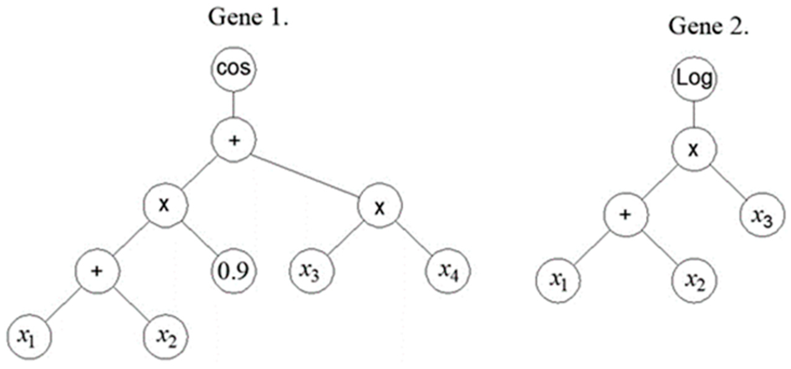
Figure 6.
Gene combination and mutation in MGGP models [25].
Figure 6.
Gene combination and mutation in MGGP models [25].
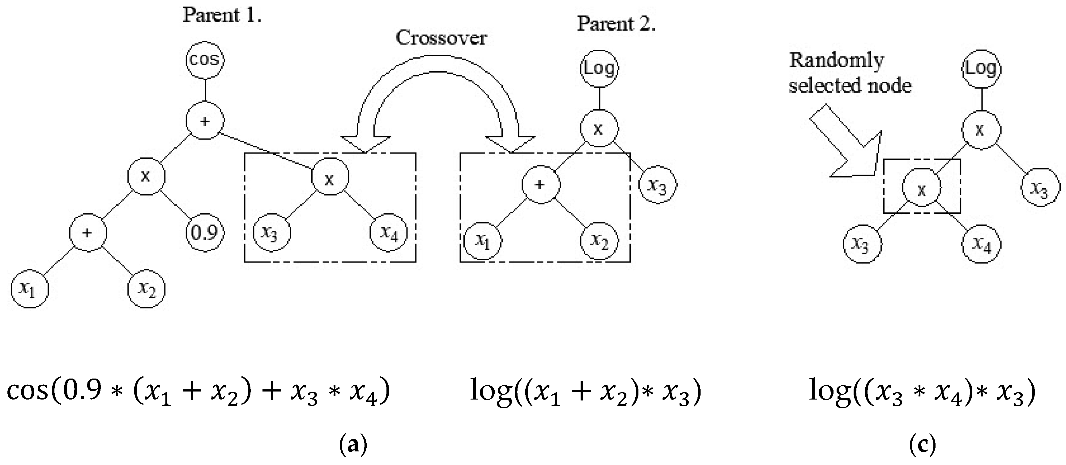
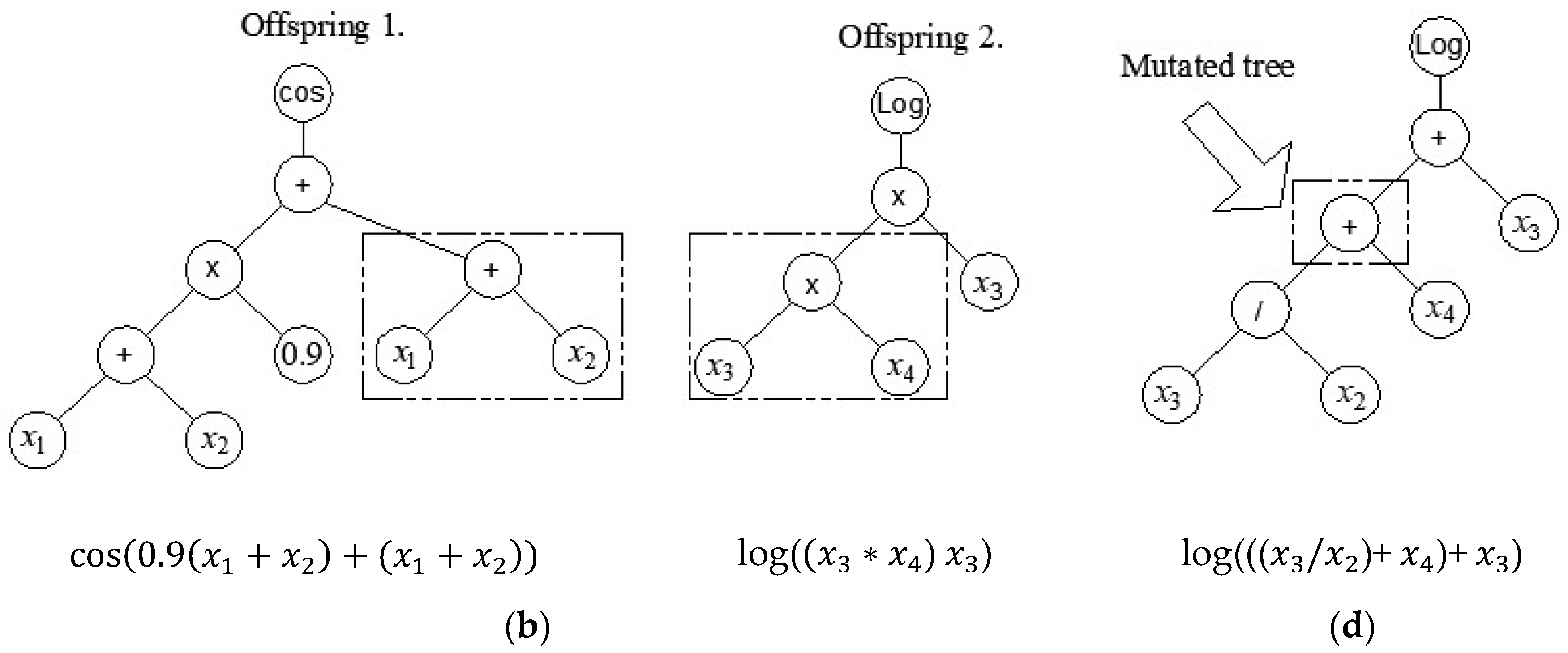
Figure 7.
Multi-layer perceptron (MLP) model [12].
Figure 7.
Multi-layer perceptron (MLP) model [12].
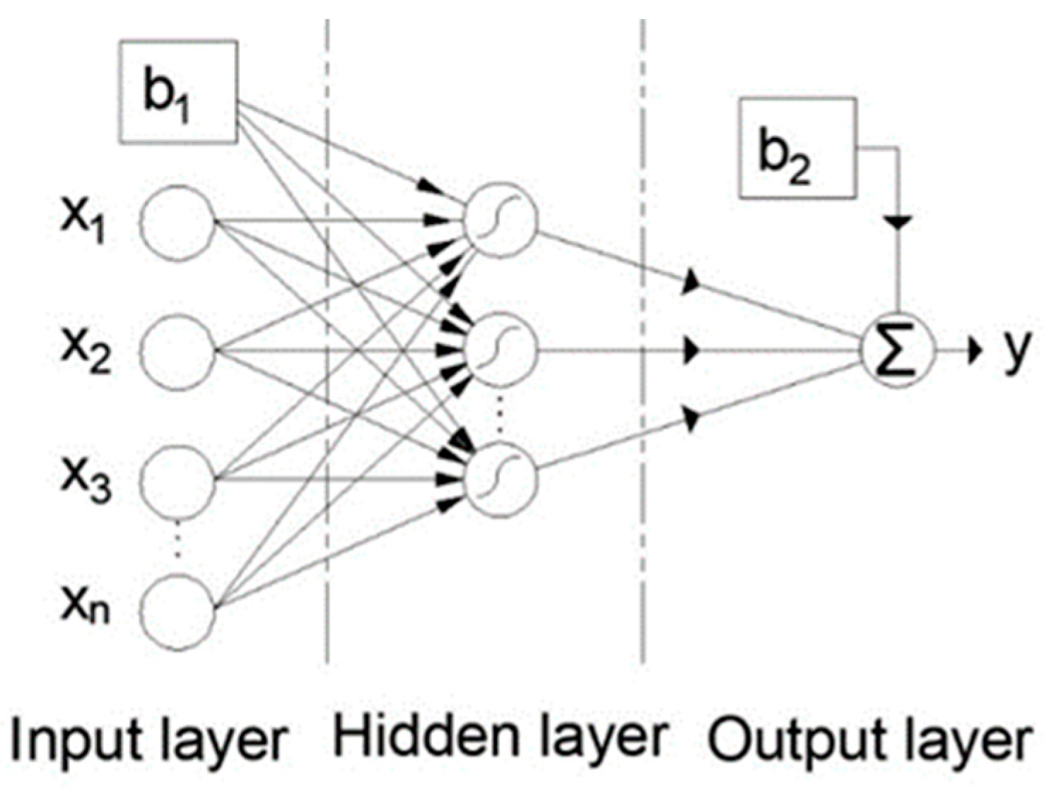
Figure 8.
Single-lap shear bond test configuration.
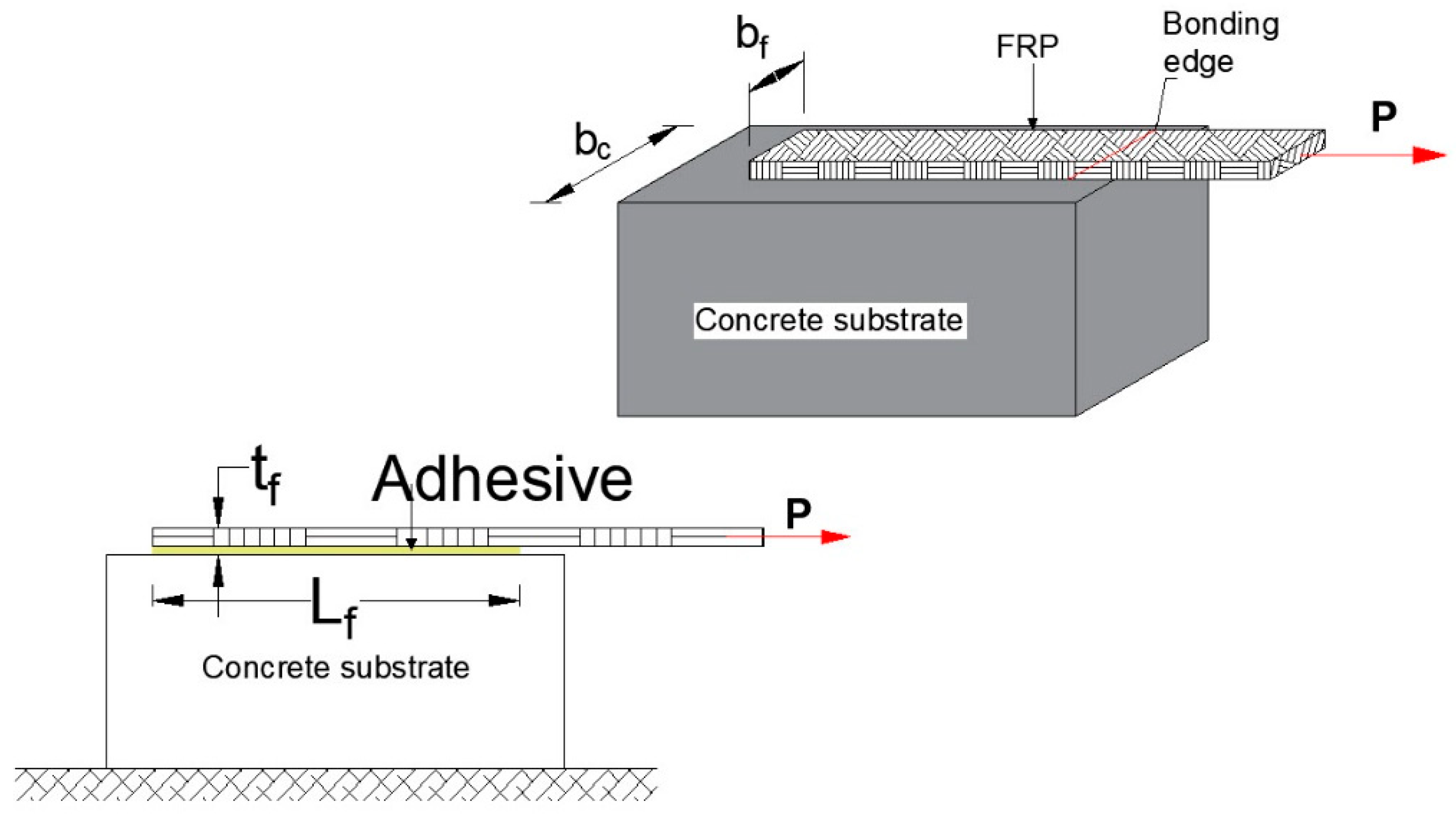
Figure 9.
Comprehensive procedure for building a machine learning model to predict the output variable (kN).
Figure 9.
Comprehensive procedure for building a machine learning model to predict the output variable (kN).
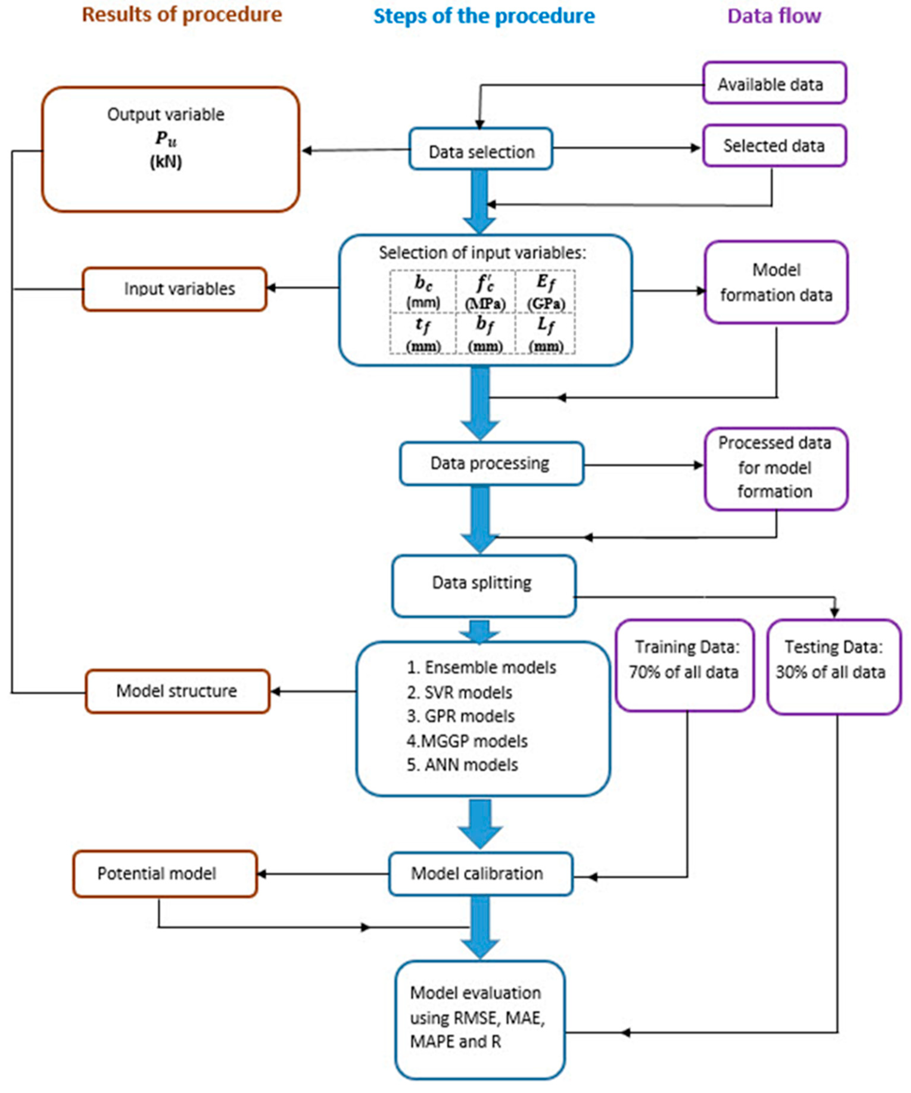
Figure 10.
Dependence of the accuracy criteria on the hyper parameters of the boosted trees models.
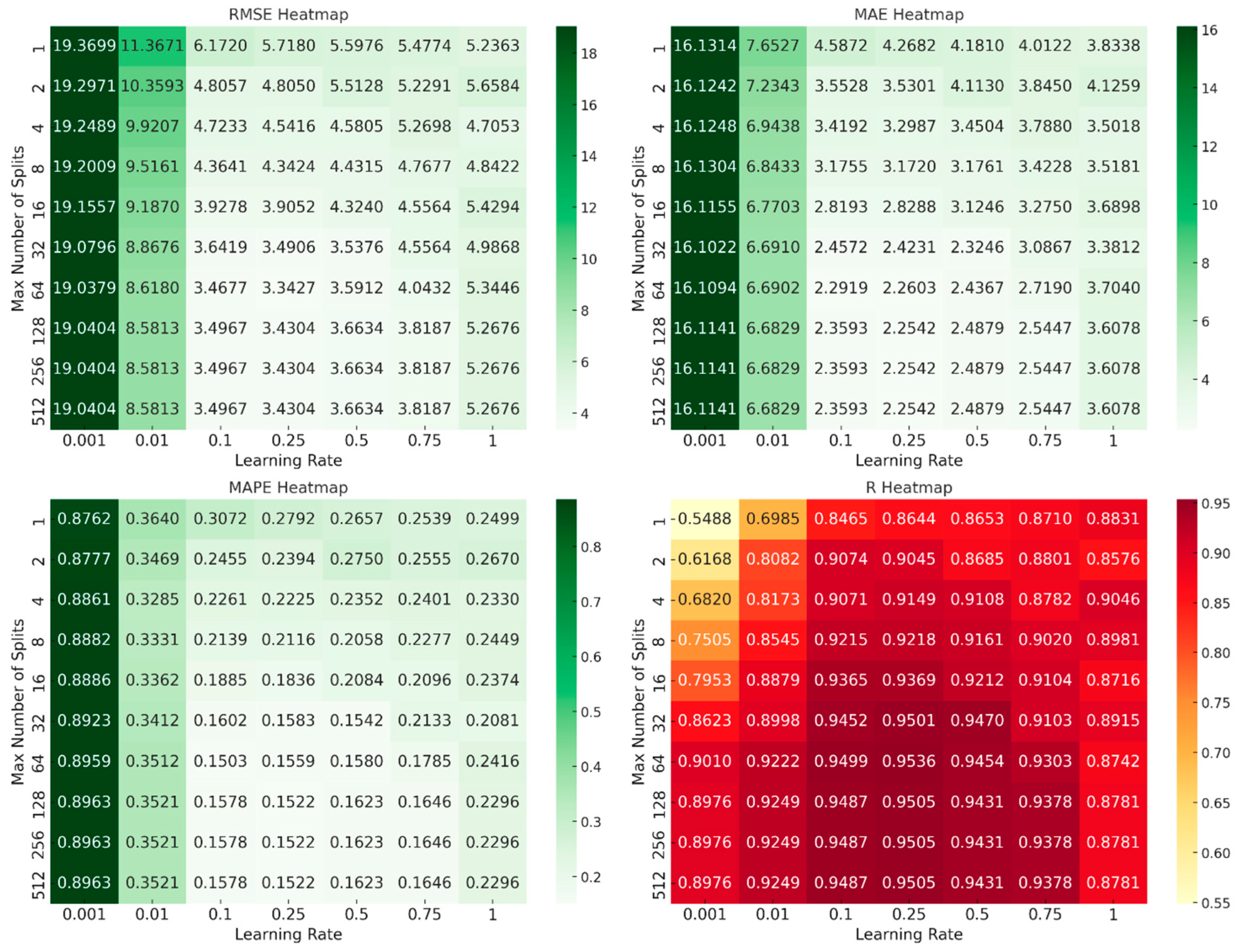
Figure 11.
Relationship between MSE and the learning rate parameter λ and number of trees in the boosted trees model.
Figure 11.
Relationship between MSE and the learning rate parameter λ and number of trees in the boosted trees model.
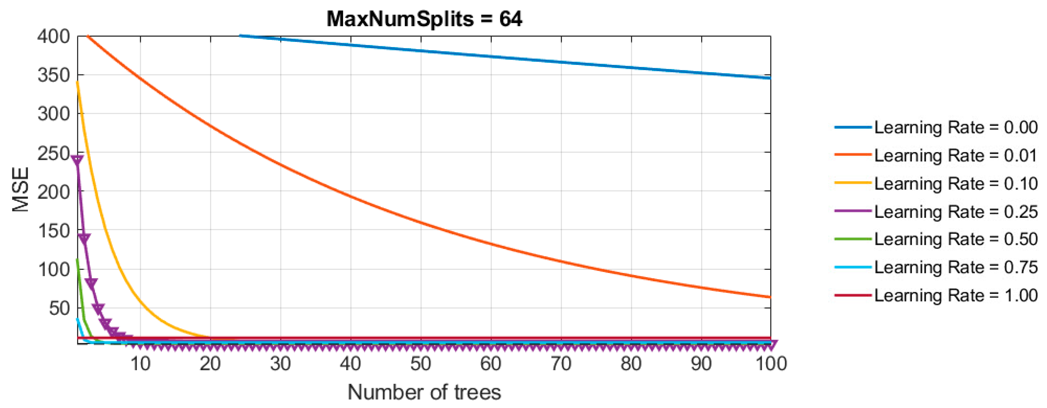
Figure 12.
Significance of input variables for boosted trees model.
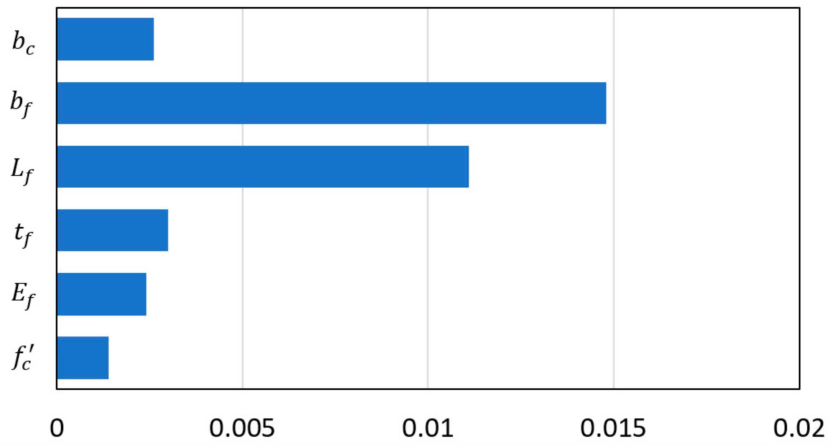
Figure 13.
Dependence of the accuracy criteria on the hyper parameters of the Random Forest and TreeBagger models.
Figure 13.
Dependence of the accuracy criteria on the hyper parameters of the Random Forest and TreeBagger models.
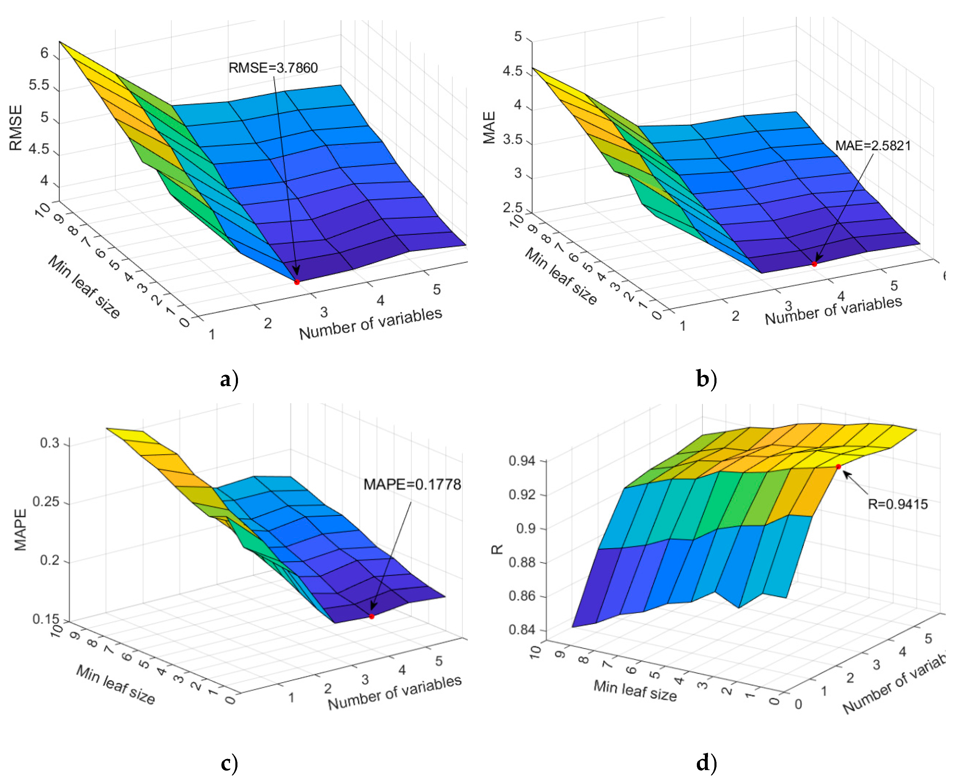
Figure 14.
Variable importance in GPR model with ARD exponential function.
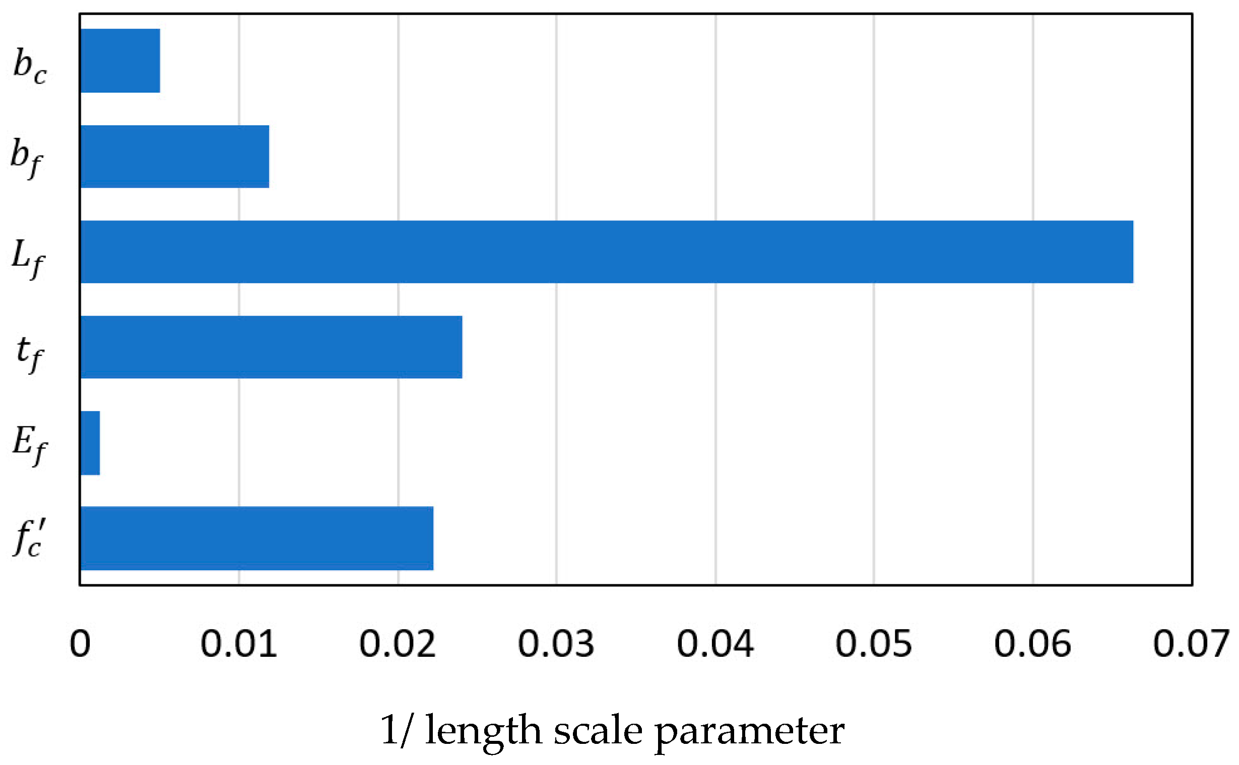
Figure 15.
Graphic representation of the Pareto front for the initial population of 800 models (individuals).
Figure 15.
Graphic representation of the Pareto front for the initial population of 800 models (individuals).
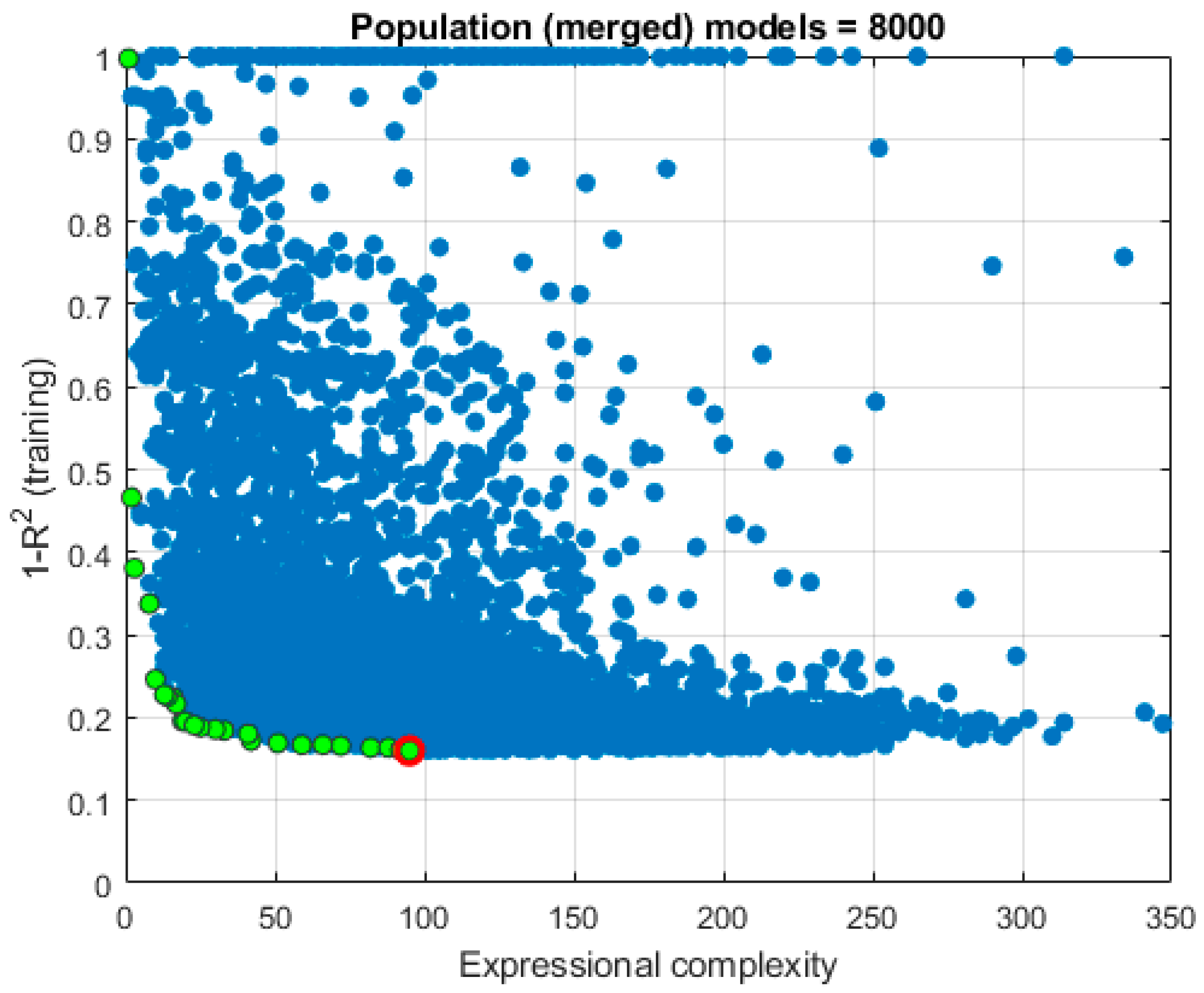
Figure 16.
Tree structure representation of genes from the optimal MGGP model.
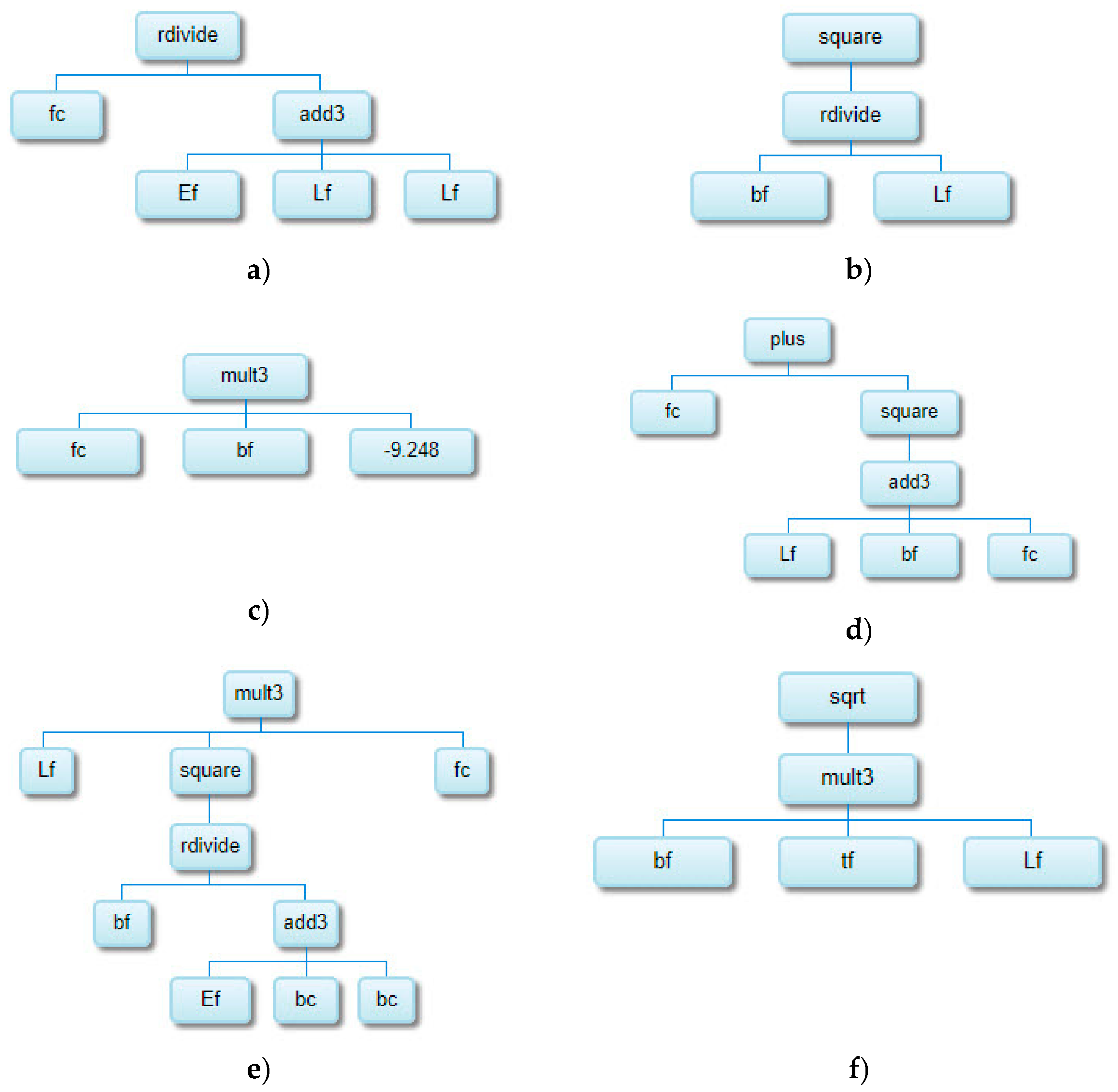
Figure 17.
Dependence of accuracy criteria on hyper parameters for the MGGP model.
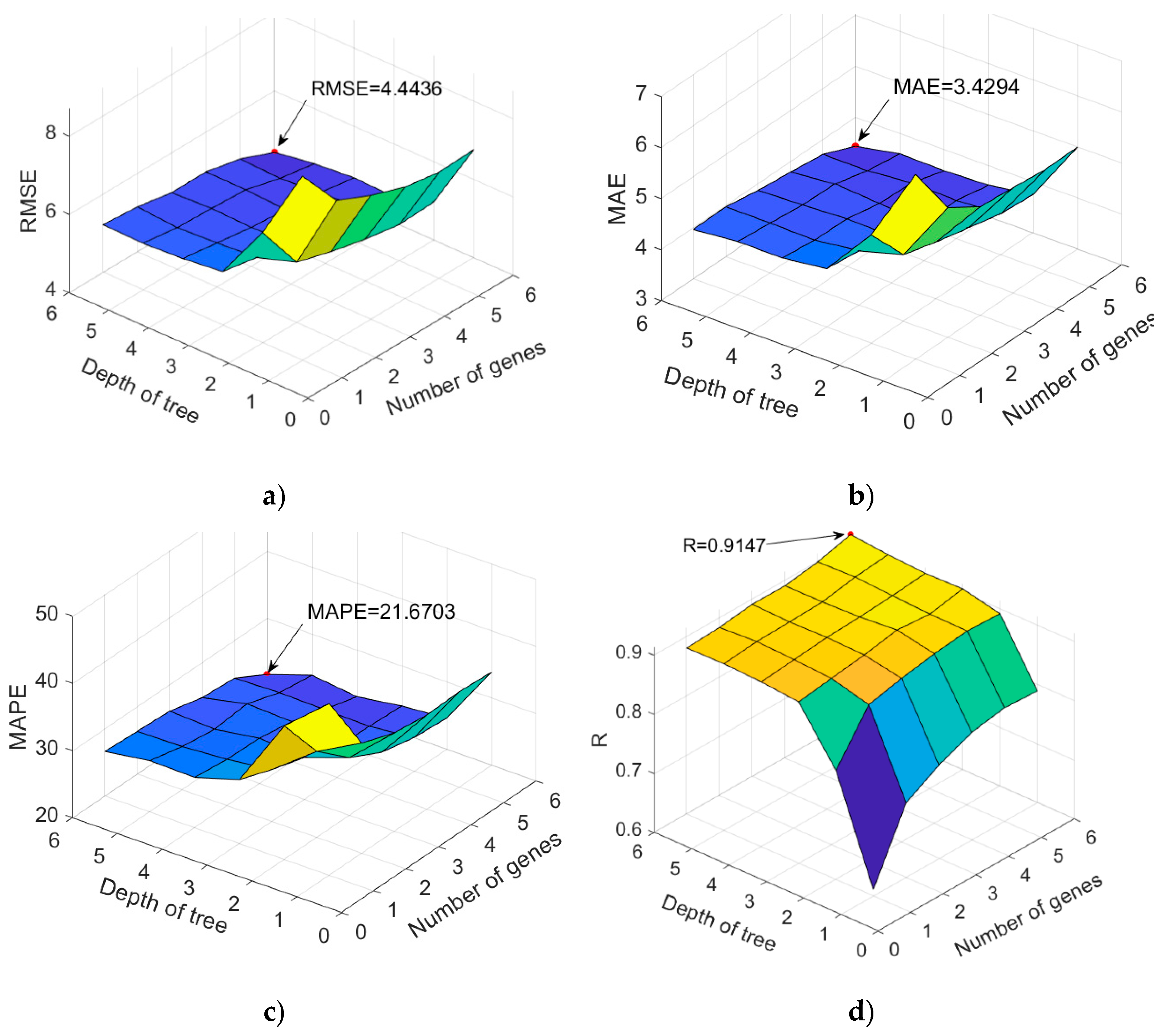
Figure 18.
Relationship between accuracy criteria and number of hidden neurons.
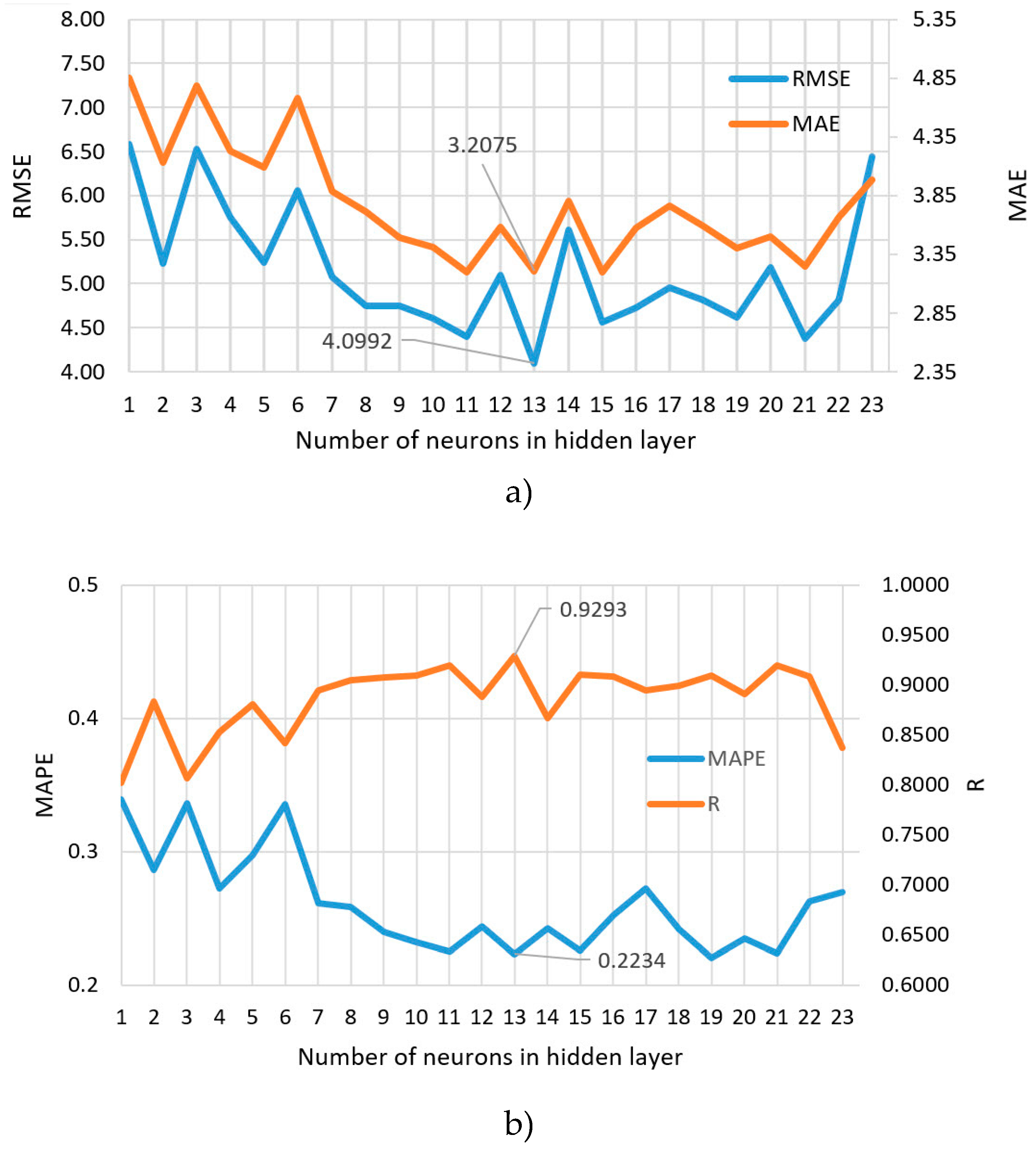
Figure 19.
Regression plot of target and predicted values for the GPR ARD Exponential model.
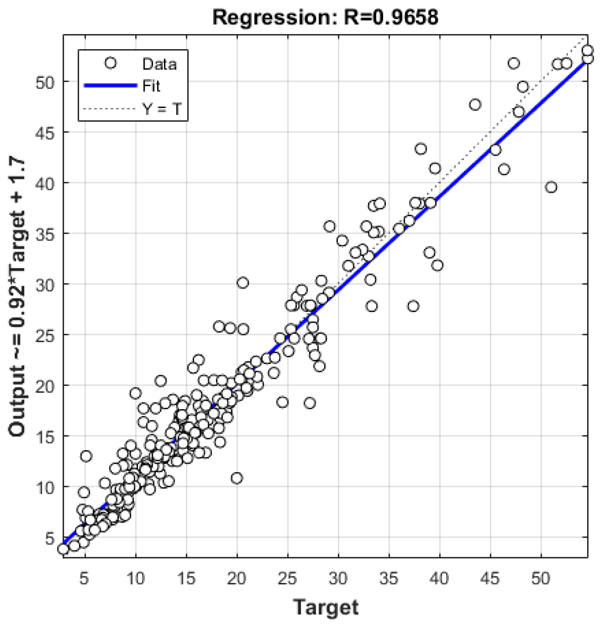
Figure 20.
Diagram of target values and predictions for the optimal GPR ARD Exponential model.
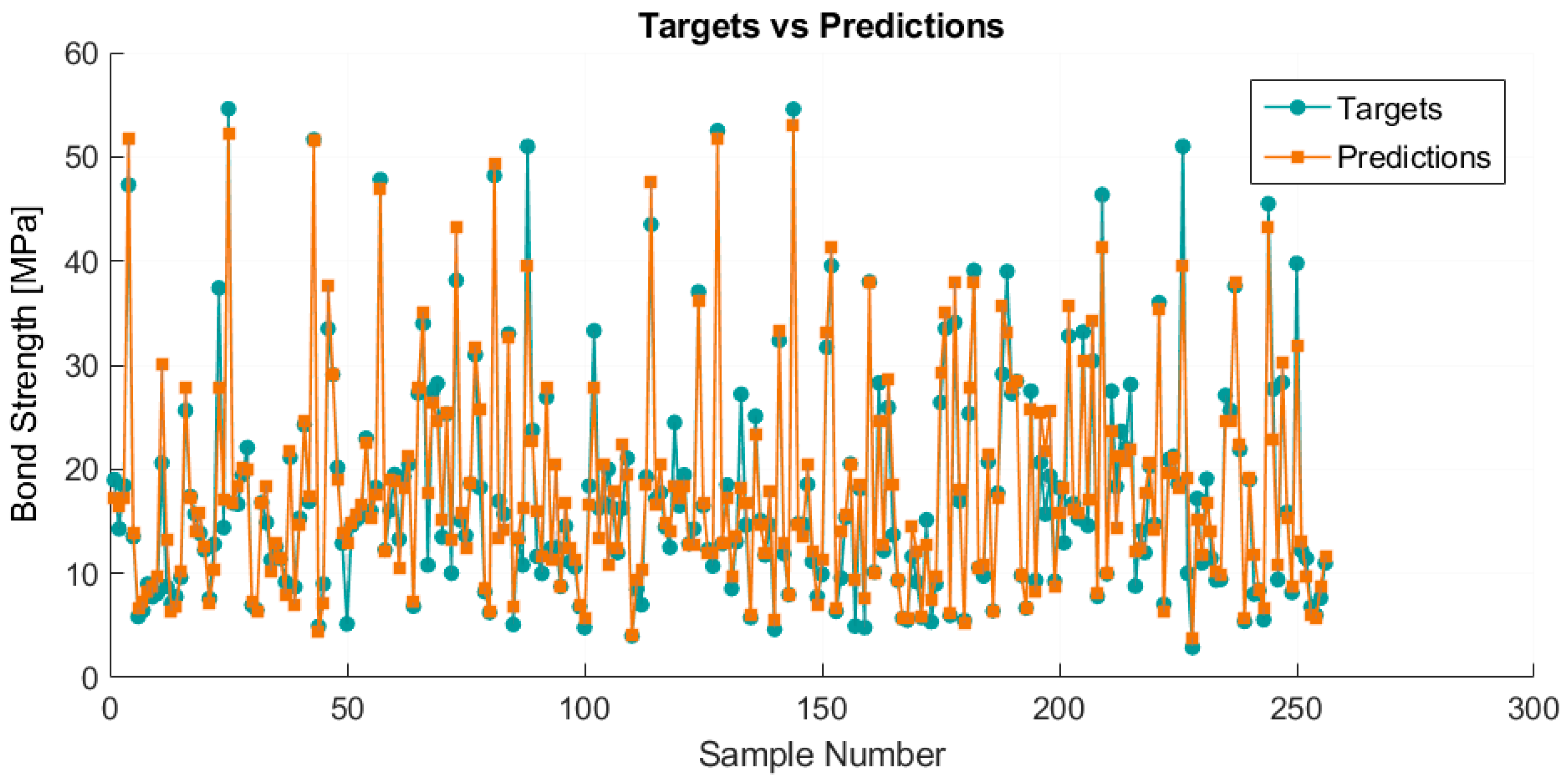
Figure 21.
MATLAB Graphical User Interface (GUI).
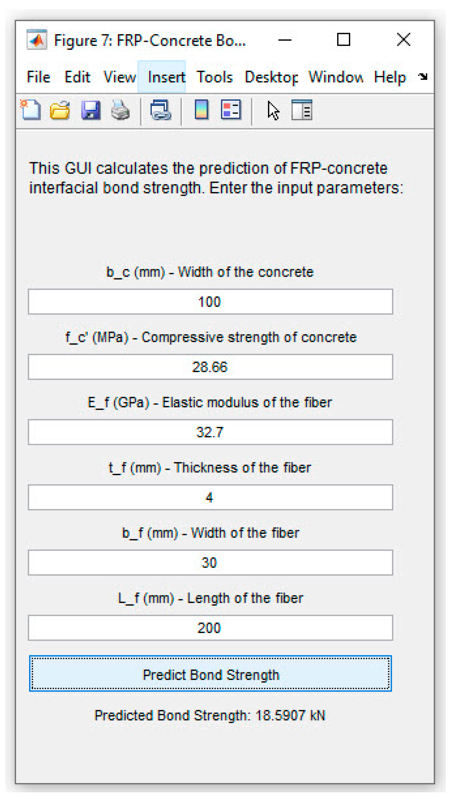

Table 1.
Comprehensive compilation of published experimental data [2].
Table 1.
Comprehensive compilation of published experimental data [2].
| Reference | Num.of tests |
(MPa) |
GPa) |
(mm) |
(mm) |
(mm) |
(mm) |
(kN) |
| Adhikary and Mutsuyoshi [27] | 7 | 24-36.5 | 230 | 0.11-0.33 | 100-150 | 100 | 150 | 16.75-28.25 |
| Bilotta et al. [28] | 29 | 21.46-26 | 170-241 | 0.166-1.4 | 100-400 | 50-100 | 150 | 17.24-33.56 |
| Bilotta et al. [29] | 13 | 19 | 109-221 | 1.2-1.7 | 300 | 60-100 | 160 | 29.86-54.79 |
| Bimal and Hiroshi [30] | 7 | 24-36.5 | 230 | 0.111-0.334 | 100-150 | 100 | 150 | 16.8-28.3 |
| Carlo et al. [31] | 14 | 58-63 | 230-390 | 0.165-0.495 | 65-130 | 50 | 100 | 12.1-29.8 |
| Chajes et al. [32] | 15 | 24-48.87 | 108.48 | 1.016 | 51-203 | 25.4 | 152.4-228.6 | 8.09-12.81 |
| Czaderski and Olia [33] | 8 | 32-33 | 165-175 | 1.23-1.68 | 300 | 100 | 150 | 43.5-56.1 |
| Dai et al. [34] | 19 | 33.1-35 | 74-230 | 0.11-0.59 | 210-330 | 100 | 400 | 15.6-51 |
| Faella et al. [35] | 3 | 32.78-37.55 | 140 | 1.4 | 200-250 | 50 | 150 | 31-39.78 |
| Fen et al. [36] | 11 | 8-36 | 240.72-356.75 | 0.111 | 50-120 | 50-100 | 150 | 7.13-17.34 |
| Hoseini and Mostofinejad [37] | 22 | 36.5-41.1 | 238 | 0.131 | 20-250 | 48 | 150 | 7.58-10.12 |
| Kanakubo et al. [38] | 12 | 23.8-57.6 | 252.2-425.1 | 0.083-0.334 | 300 | 50 | 100 | 7-25.6 |
| Kamiharako et al. [39] | 17 | 34.9-75.5 | 270 | 0.111-0.222 | 100-250 | 10-90 | 100 | 3.1-14.9 |
| Ko et al. [40] | 13 | 27.7-31.4 | 165-210 | 1-1.4 | 300 | 60-100 | 150 | 27.5-56.5 |
| Liu [41] | 57 | 16-51.6 | 272.66 | 0.167 | 50-300 | 50 | 100 | 10.97-23.87 |
| Lu et al. [42] | 3 | 47.64-64.08 | 230-390 | 0.22-0.501 | 200-250 | 40-100 | 100-500 | 14.1-38 |
| Maeda et al. [43] | 5 | 40.8-44.91 | 230 | 0.11-0.22 | 65-300 | 50 | 100 | 5.8-16.25 |
| Nakaba et al. [44] | 41 | 24.41-65.73 | 124.5-425 | 0.167-2 | 250-300 | 40-50 | 100 | 8.73-27.24 |
| Pham and Al-Mahaidi [45] | 23 | 44.57 | 209 | 0.176 | 60-220 | 70-100 | 140 | 18.8-42.8 |
| Ren [46] | 28 | 22.96-46.07 | 83.03-207 | 0.33-0.507 | 60-150 | 20-80 | 150 | 4.61-22.8 |
| Savoia and Ferracuti [47] | 14 | 52.6 | 165-291.02 | 0.13-1.2 | 200-400 | 50-80 | 150 | 14.4-41 |
| Savoia et al. [48] | 20 | 26 | 180-241 | 0.166-1.2 | 100-400 | 80-100 | 150 | 18.97-40 |
| Sharma et al. [49] | 24 | 23.76-28.66 | 32.7-300 | 1.2-4 | 100-300 | 30-50 | 100 | 12.5-46.35 |
| Tan [50] | 6 | 30.8 | 97-235 | 0.111-0.169 | 70-130 | 50 | 100 | 6.46-11.43 |
| Täljsten [51] | 5 | 41.2-68.33 | 162-170 | 1.2-1.25 | 100-300 | 50 | 200 | 17.3-35.1 |
| Takeo et al. [52] | 25 | 24.7-29.25 | 230-373 | 0.111-0.501 | 100-300 | 40 | 100 | 6.75-14.35 |
| Toutanji et al. [53] | 10 | 17.0-61.5 | 110 | 0.495-0.99 | 100 | 50 | 200 | 11.64-19.03 |
| Ueda et al. [54] | 15 | 23.79-48.85 | 230-372 | 0.11-0.55 | 65-300 | 10-100 | 100-500 | 2.4-38 |
| Ueno et al. [55] | 40 | 23-74.5 | 42.625-43.537 | 1.03-1.8 | 200-230 | 40 | 80 | 9.52-18.29 |
| Wu and Jiang [56] | 65 | 25.3-59.02 | 238.1-248.3 | 0.167 | 30-400 | 50 | 150 | 7.38-30.15 |
| Wu et al. [57] | 22 | 65.73 | 23.9-390 | 0.083-1 | 250-300 | 40-100 | 100 | 11.8-27.25 |
| Woo and Lee [58] | 51 | 24-40 | 152.2 | 1.4 | 50-300 | 10-50 | 200 | 4.55-27.8 |
| Xu et al. [59] | 24 | 24.1-70 | 230 | 0.17-0.84 | 50-300 | 30-70 | 100 | 7.8-31.13 |
| Yao [60] | 59 | 19.12-27.44 | 22.5-256 | 0.165-1.27 | 75-240 | 25-100 | 100-150 | 4.75-19.07 |
| Yuan et al. [61] | 1 | 23.79 | 256 | 0.165 | 190 | 25 | 150 | 5.74 |
| Zhang et al. [62] | 20 | 38.9-43.5 | 94-227 | 0.262-0.655 | 250 | 50-150 | 200-250 | 13.03-52.49 |
| Zhao et al. [63] | 5 | 16.4-29.36 | 240 | 0.083 | 100-150 | 100 | 150 | 11-12.75 |
| Zhou [64] | 102 | 48.56-74.67 | 71-237 | 0.111-0.341 | 20-200 | 15-150 | 150 | 3.75-28 |
Table 2.
Statistical summary and descriptive characteristics of variables in the training Set.
|
(mm) |
(MPa) |
(GPa) |
(mm) |
(mm) |
(mm) |
(kN) |
|
| min | 80.00 | 8.00 | 22.50 | 0.08 | 10.00 | 20.00 | 2.40 |
| max | 500.00 | 74.67 | 425.10 | 4.00 | 150.00 | 400.00 | 56.50 |
| average | 144.31 | 39.38 | 203.66 | 0.50 | 57.62 | 175.42 | 17.80 |
| mode | 150.00 | 48.56 | 230.00 | 0.17 | 50.00 | 100.00 | 11.90 |
| median | 150.00 | 36.50 | 230.00 | 0.17 | 50.00 | 150.00 | 15.73 |
| std | 56.93 | 15.23 | 77.97 | 0.53 | 26.57 | 102.31 | 10.13 |
Table 3.
Statistical summary and descriptive characteristics of variables in the test Set.
|
(mm) |
(MPa) |
(GPa) |
(mm) |
(mm) |
(mm) |
(kN) |
|
| min | 56.93 | 8.00 | 22.50 | 0.08 | 10.00 | 20.00 | 2.40 |
| max | 500.00 | 74.67 | 425.10 | 4.00 | 150.00 | 400.00 | 56.50 |
| average | 144.84 | 38.94 | 208.34 | 0.53 | 57.50 | 180.23 | 18.55 |
| mode | 150.00 | 65.73 | 230.00 | 0.17 | 50.00 | 100.00 | 12.75 |
| median | 150.00 | 36.27 | 230.00 | 0.17 | 50.00 | 162.50 | 16.47 |
| std | 68.25 | 15.03 | 75.95 | 0.58 | 25.21 | 105.20 | 9.85 |
Table 4.
Detailed regression results: Estimates, Standard Errors, t-Statistics, and p-Values for model parameters.
Table 4.
Detailed regression results: Estimates, Standard Errors, t-Statistics, and p-Values for model parameters.
| Parameter | Estimate | Standard Error | tStat | pValue |
| (Intercept) | -15.9200 | 2.8688 | -5.5492 | 4.3568× |
| -0.0393 | 0.0138 | -2.8525 | 0.0045 | |
| 0.3682 | 0.0702 | 5.2473 | 2.1625× | |
| 0.0695 | 0.0098 | 7.0878 | 3.9461× | |
| 0.0654 | 0.0476 | 1.3739 | 0.1700 | |
| 0.0574 | 0.0112 | 5.1353 | 3.8429× | |
| 0.0443 | 0.0054 | 8.2612 | 9.6963× | |
| 0.0014 | 0.0002 | 6.0212 | 3.0620× | |
| 0.1313 | 0.0145 | 9.0761 | 1.7139× | |
| -0.0005 | 0.0001 | -3.9565 | 8.5421× | |
| -0.0001 | 0.0001 | -2.4285 | 0.0155 | |
| -0.0025 | 0.0007 | -3.3629 | 8.2189× | |
| -0.0001 | 0.0000 | -4.3966 | 1.3068× | |
| -0.0009 | 0.0002 | -3.8854 | 1.1386× | |
| -0.00007 | 0.0000 | -3.4915 | 5.1660× |
Table 5.
Comparative analysis of results using linear, RBF and sigmoid kernel in SVR method.
| Model | RMSE | MAE | MAPE/100 | R |
| Lin. kernel | 8.7154 | 6.6468 | 0.2105 | 0.7751 |
| RBF kernel | 4.9646 | 3.5352 | 0.1171 | 0.9332 |
| Sig. kernel | 8.7104 | 6.6094 | 0.2073 | 0.7718 |
Table 6.
Parameters of GPR model covariance functions.
| GP Model Covariance Function | Covariance Function Parameters | |||
| Exponential | ||||
| 48.8828 | 35.9025 | |||
| Squared Exponential | ||||
| 1.1564 | 11.6670 | |||
| Matern 3/2 | ||||
| 1.9430 | 12.5620 | |||
| Matern 5/2 | ||||
| 1.6073 | 12.0472 | |||
| Rational Quadratic | ||||
| 1.9747 | 0.0057 | 39.8560 | ||
where .
Table 7.
Parameters of GPR ARD model covariance functions.
| Covariance Function Parameters | |||||
| ARD Exponential: ;=44.4870; =0.8339 | |||||
| 45.0052 | 813.3275 | 41.5953 | 15.0703 | 83.9007 | 199.8780 |
| ARD Squared exponential: =13.0762 | |||||
| 0.1181 | 6.1165 | 0.1452 | 0.3453 | 2.0239 | 1.5321 |
| ARD Matern 3/2: =11.8722 | |||||
| 0.4342 | 10.3369 | 0.8032 | 0.2128 | 1.7551 | 3.0059 |
| ARD Matern 5/2: =11.2938 | |||||
| 0.2738 | 8.1979 | 0.6294 | 0.1177 | 1.1174 | 2.2108 |
| ARD Rational quadratic: =0.0082; =40.2700 | |||||
| 1.2252 | 23.3200 | 1.2758 | 0.3892 | 2.1230 | 5.8575 |
where .
Table 8.
Comparative analysis of results without using ARD.
| Model | RMSE | MAE | MAPE/100 | R |
| Exp. | 3.2790 | 2.1928 | 0.1498 | 0.9558 |
| Sq.Exp. | 3.8110 | 2.6042 | 0.1794 | 0.9395 |
| Mattern 3/2 | 3.5651 | 2.3879 | 0.1632 | 0.9475 |
| Mattern 5/2 | 3.6651 | 2.4752 | 0.1697 | 0.9443 |
| Rat.Quadratic | 3.3152 | 2.2421 | 0.1593 | 0.9551 |
Table 9.
Comparative analysis of results using ARD.
| Model | RMSE | MAE | MAPE/100 | R |
| ARD Exp. | 2.9039 | 1.8953 | 0.1257 | 0.9650 |
| ARD Sq.Exp. | 3.4447 | 2.3562 | 0.1590 | 0.9511 |
| ARD Mattern 3/2 | 2.8671 | 1.9319 | 0.1329 | 0.9658 |
| ARD Mattern 5/2 | 3.0073 | 2.0360 | 0.1410 | 0.9623 |
| ARD Rat.Quadratic | 2.9167 | 1.9377 | 0.1323 | 0.9647 |
Table 10.
The parameters seting for MGGP models.
| Parameter | Setting |
| Function set | times, minus, plus, rdivide, square, exp, log, mult3, sqrt, cube, power |
| Population size | From 100 to 1000 with step 100 |
| Number of generations | 1000 |
| Max number of genes | 6 |
| Max tree depth | 6 |
| Tournament size | 2 |
| Elitism | 0.05% of population |
| Crossover probability | 0.84 |
| Mutation probability | 0.14 |
| Probability of Pareto tournament | 0.70 |
Table 11.
Analytical expressions for the genes of the optimal model of the Pareto front for the initial population of 800 models.
Table 11.
Analytical expressions for the genes of the optimal model of the Pareto front for the initial population of 800 models.
Table 12.
Accuracy criterion values for 10 models on the Pareto front.
| Model ID | Model complexity |
RMSE | MAE | MAPE/100 | R |
| 7961 | 95 | 4.4436 | 3.4294 | 0.2167 | 0.9147 |
| 7570 | 92 | 4.6349 | 3.6170 | 0.2417 | 0.9079 |
| 1766 | 82 | 4.8264 | 3.7418 | 0.2456 | 0.9004 |
| 3867 | 88 | 4.8137 | 3.7101 | 0.2404 | 0.9004 |
| 7161 | 72 | 4.5985 | 3.5375 | 0.2362 | 0.9095 |
| 7164 | 66 | 4.6936 | 3.6328 | 0.2407 | 0.9056 |
| 7167 | 59 | 4.6545 | 3.5922 | 0.2383 | 0.9056 |
| 6726 | 51 | 4.6894 | 3.5855 | 0.2383 | 0.9059 |
| 6959 | 42 | 4.6829 | 3.5373 | 0.2292 | 0.9061 |
| 7292 | 41 | 4.9642 | 3.7915 | 0.2514 | 0.8941 |
Table 13.
Analytical expressions for the genes of the Model 6959 of the Pareto front for the initial population of 800 models.
Table 13.
Analytical expressions for the genes of the Model 6959 of the Pareto front for the initial population of 800 models.
|
|
|
Table 14.
Parameter settings for model calibration in MATLAB.
| Parameter | Value |
| Epoch limit | 1000 |
| MSE target (performance) | 0 |
| Gradient limit | 1.00 × |
| Mu value | Range from 0.005 to 1.00 × |
Table 15.
Comparative analysis of all optimal analyzed models based on selected accuracy criteria.
| Model | RMSE | MAE | MAPE/100 | R |
| Linear with interaction | 4.9278 | 3.8491 | 0.2748 | 0.8955 |
| Gradient Boosted | 3.3427 | 2.2603 | 0.1559 | 0.9536 |
| Random Forest (64 splits) | 3.7860 | 2.5821 | 0.1778 | 0.9415 |
| TreeBagger | 3.8302 | 2.5847 | 0.1790 | 0.9399 |
| SVR RBF | 4.9646 | 3.5352 | 0.1171 | 0.9332 |
| GPR Exponential | 3.2790 | 2.1928 | 0.1498 | 0.9558 |
| GPR ARD Exponential | 2.8671 | 1.9319 | 0.1329 | 0.9658 |
| MGGP | 4.4436 | 3.4294 | 0.2167 | 0.9147 |
| MGGP simplified | 4.6829 | 3.5373 | 0.2292 | 0.9061 |
| NN 6-13-1 | 4.0992 | 3.2075 | 0.2234 | 0.9293 |
Disclaimer/Publisher’s Note: The statements, opinions and data contained in all publications are solely those of the individual author(s) and contributor(s) and not of MDPI and/or the editor(s). MDPI and/or the editor(s) disclaim responsibility for any injury to people or property resulting from any ideas, methods, instructions or products referred to in the content. |
© 2024 by the authors. Licensee MDPI, Basel, Switzerland. This article is an open access article distributed under the terms and conditions of the Creative Commons Attribution (CC BY) license (http://creativecommons.org/licenses/by/4.0/).
Copyright: This open access article is published under a Creative Commons CC BY 4.0 license, which permit the free download, distribution, and reuse, provided that the author and preprint are cited in any reuse.


