
Submitted:
22 November 2024
Posted:
23 November 2024
You are already at the latest version
Abstract
Performance analysis, utilizing video technology and recent technological advancements in soccer stadiums, provides a wealth of data, including player trajectories and real-time game statistics, which are crucial for tactical evaluation and decision-making by coaches and players. This data allows for the definition of metrics that not only enriches the experience for soccer fans through enhanced visual displays, but also empowers coaching staff and managers to make informed, real-time decisions that directly impact match outcomes. Ultimately, it serves as a pivotal tool for improving team strategy based on comprehensive post-match data analysis. In this article, we present a mathematical model to study the concept of pressure between players and, subsequently, between teams. We first explore the concept in a fixed frame of a match, determining what we call {\sl influence areas} between players. We introduce the unit pressure function and analyze the total number of pressure interactions. Then, we apply these concepts to football matches, considering various factors such as players and the radius of the area of influence, examining pressure efficiency through mean unitary pressure. Lastly, a real case study is presented, showcasing visualizations like a heatmap matrix displaying individual and collective pressure, as well as team pressure balance.
Keywords:
Mathematical Modeling
; Approximation Functions
; Football metrics
; Pressure model
; Tracking data analysis
1. Introduction
Top-level soccer is an increasingly competitive sport and, as a consequence, performance analysis is becoming an important tool for supporting coaches and players in the decision-making process, providing relevant information about the play. For decades, the use of video has been a key element in the tactical analysis of teams before and after a match [1]). The technological advances developed in recent years in soccer stadiums now make it possible to obtain a large amount of data related to the game, both individually and collectively. These data, which contain the trajectories of the players, the ball or the movement of the refereeing team in real time, allow a very precise mathematical analysis of the parameters that characterize the course of the matches. In addition, broadcasters have realized that coverage of sporting events can be enhanced by providing analysis of the action, often by specialized professionals who use visual tools and dashboards to describe key events and sequences during the game. There is also an apparent consumer appetite for statistics and attractive visual data displays, and there are many websites dedicated to providing this type of information. Therefore, there is a general interest in improving the visualizations and filling them with technical content that can provide more information to soccer fans. But this is not only of interest to the fans, but also to the coaching staff and managers, who can analyze the data, even in real time, and make relevant decisions that will affect the outcome of the match. It is thus intended to give a tool for improving the strategy of the teams, based on real data, after processing the complete data describing the match.
The basic ways to obtain the real trajectories and positions of objects and players are mainly achieved by Electronic Performance and Tracking Systems (EPTS). Technologies based on Optical Tracking System (OTS) capture and can analyze 25 frames per second, which would already add up to a total of sets of values for 90 minutes of play per game, and if we consider 22 players, a game ball and the referee team constitute a big-data of the order of data vectors in euclidean space to be stored, which are not very feasible to analyze without an adequate modelling and treatment to obtain relevant and useful information for potential customers of use.
The are widely used indicators such as shots on goal, number of passes, tackle rates, team ball possession and distances covered although their use is a matter of question [2]. Then, it is a task of data science to derive indicators from raw data that describe relevant situations of the game properly ([3]). In particular, a lot of studies have analysed tactical indicators related to goal scoring in soccer (see for example [4]). In some of them, one of the concepts that recursively appears when we talk about football is the concept of pressure. Several attempts to define pressure can be found in the literature. In 1996 [5] introduce the minimum moving time pattern (MMT) of a player at any one moment as a pattern in which each point has the minimum time to move from that player’s current position to that point; and also defined the dominant region of a player at any one moment as a region where the player can arrive at earlier than all of the others.
The concept of playing style is discussed in the reference [6], with special emphasis on what variables can be measured to determine it. In particular in attacking or offensive phases of play players move into positions towards the zones of the field in order to receive the ball or score a goal and is in this phases of the play when presion, considered as limiting the passing options and limiting space available, becomes fundamental.
One of the most characteristic and essential elements of soccer defense is pressing but it has not yet received much attention from researchers in football analytics. In [7] authors analyze the automatically extraction of football events using tracking data that implies among others fact the definition of the possession of the ball to determine in-game events. For this purpose they develop a decision tree-based algorithm and in the conclusions they establish as an improvement of their algorithm extending the possession zone definition to encompass a variable radius/shape based on pitch location, proximity of opponents and player velocity. The concept of pressure (which is directly related to that of possession) proposed in this article is based on the concept of this zone around the player and addresses, among other things, the determination of this radius.
[8] proposed a computational approach to detecting and quantifying the relationships of pressure and pressing behavior emerging during a game. To support examination of team tactics in different situations, they designed and implemented an interactive visual tool named time mask that enables selection of multiple disjoint time intervals in which given conditions are fulfilled.
In 2019 [9] studied as well an approach to quantification of attacking performance in football. Their procedure determined a quantitative representation of the probability of a goal being scored for every point in time at which a player is in possession of the ball they refereed to this as dangerousness. This parametric variable was determined by means of four variables, one of them denoted as pressure which represents the possibility that the defending team prevent the player from completing an action with the ball. In determining the pressure, they assumed that a defender exerts pressure when his distance from the player is bellow some threshold value. They provided a pressure zone with covers four sub-areas with different radii which result of the angle between player and the centre of the goal. This model for defining pressure results in a rather complex formula.
In [10], in the context of tactical key performance indicators, authors introduced the Pressure Passing Efficiency Index (PPEI). It is based on the number of outplayed opponents. It aims to measure high quality through-balls by weighing passes with more than one outplayed opponent by the pressure on both pass initiator and receiver.
In [11] author introduces a novel metric to quantify its effectiveness in different contexts. He assess pressure calculating probabilities of recovering the ball and conceding a goal-scoring opportunity in the near future. They XGBoost stacked with a logistic regression model to estimate probabilities.
In [12] authors explore the area of defensive performance in football by analyzing successful defensive phases using space and time characteristics of defensive pressure. They use data from German Bundesliga games. The study distinguishes pressure on the ball-carrier, the group of attackers closest to the ball, and the entire team, finding that pressure is higher in areas closer to the ball and as the defensive play approaches its end.
In this paper we have applied our definition of pressure to the analysis of data from a real football match. These data have been obtained from Metrica company ([13]). These are two games which have been anonymized, meaning there are no references to the names of players, teams or competitions. The dimensions of the field are the same for both games: meters and tracking and event data are synchronized. A detailed information is given about the definition and explanation of all events types and subtypes.
The article is organized as follows. After this introductory section in the second one we first study the notions of pressure on a fixed frame of the match. To do that we start by introducing the concept of influence area () between two players. This function depends of the distance between the players and also on the ball radius. An approximation of this function (by using a secant line) gives the definition of pressure () between the players. This notion allows us to define the pressure between one team over a player and finally between the two teams. Since the cumulative pressure values can be very large then we introduce the unit pressure function (p) which it is computed by dividing the pressures by its maximum. Then we study the total number of pressure interactions. In the final part of this section we apply the previous formulas to study the pressure on a complete match of football. Now the pressure depends, not only on the players and on the ball radius, but also on the frame. We divide this section in three parts. In the first one we determine a ball radius in order to have a significant (but not too many) number of pressure interactions. Once this value () is fixed we study the pressure along a set of frames (): the key point here is that we sum the pressures of all players defending the ball. Since in a match not all the players play the same time in the third part of this section we study the efficiency of the pressure by introducing the mean unitary pressure ( ). This provides a number in easier to use. In the third section we present a real case study providing different visualizations using our formulas. Hence we start by showing a heatmap matrix that allows us to give (in the same table) the individual and the collective pressure (both exerted and received). In the second part a Butterfly Chart (also called Tornado Chart) is presented. This visualization allows us to study the balance of pressures of the teams of the match. In the last section we discuss the results and arrive to some conclusions.
2. Materials and Methods
2.1. Pressure Functions on a Frame of a Match
Let A and B the two teams on the pitch. In this section we first introduce the notion of pressure between the players and and also the corresponding one between one team on a player and also between the two teams. In order to simplify the computations an approximation of these functions—using a secant line—will be also given. Next we introduce the unitary concepts of pressure and we finish this section by providing the total number of pressing interactions.
Throughout this section we set a frame so there is no time dependence and the definitions depend only on the radius of the ball. In the next section we will use our results to analyze a complete match—with the corresponding time/frame dependence—and we will also look at how to determine the radius to compare the pressure between players and teams. We start by defining the notion of influence area between two players.
Definition 2.
Fixed a real number . We define theinfluence area between the players and , as the truncated area of the intersections balls . That is,
where is the euclidean distance, , and a and b stands for the coordinates of each player—in —.
Note that the objective of making the influence area function equal zero when is to take into account that when two players are far away enough this area cannot be considered. Figure 1 shows the truncated intersection areas between the balls and —that is the influence area between the players a and b—.
Thinking on the real-time computations we can approximate the influence area function on the interval by the secant line from to . This provides our notion of pressure.
Definition 2.
We define, for , thepressure exerted by player over the player as
The linear approximation provided in this case gives accurate results. In fact, it allows us to approximate the influence area function with small errors. Figure 2 shows a visualization of how the influence area and the pressure functions behaves for different values of r. With all this approximations we will speed up the calculations so that we can display the results dynamically in near real time.
In a similar way we can define the pressure between team and player and between two teams.
Definition 2.
Given , thepressure exerted by team over the player is defined as
Definition 2.
Fixed , thepressure exerted by team over the team is defined by
Note that some (actually many) players in will exert zero pressure—over the player —. In this case , and then (many) terms of the sum will be null.
Sometimes, in order to show the results and make them more understandable—note that the cumulative values can be, in general, very large—, it is interesting to use the unit pressure, which is denoted by the small letter . To define it recall the values of the pressure for the three singular situations given by r and are
To define the unit pressure it is enough to divide the pressure function by its maximum value, —that is the area of the circumference of radius r—:
We finish this section by counting the number of players of a team exerting pressure—in the sense that de pressure is different to zero—.
Definition 2.
Let . We will write for the number of players on team A who exerts (non null) pressure over the player . In other words it is defined by:
We define thetotal number of pressure interactionson the pitch as
Finally just observe that, the total number of interactions computed from each side—the pressure that all the members of B receive from the players of A, and the pressure that the members of A exert over the team B—coincide. This can be understood—and proved—by applying graph theory just thinking on two disjoint sets representing a graph consisting of vertices and N edges—see Figure 3—.
2.2. Modelling the Pressure in a Complete Football Match
Now we will use the formulas introduced in the previous section in order to analyze the pressure in a complete match. As a starting point we take a set of frames . Note that now our pressure definitions depend on the frame —since the distance between a and b depends actually of —. To simplify our notation we write
Of course if any of the players are not on the pitch in the frame then is defined as zero.
Step 1. Determining the radius. In order to obtain a useful tool to analyze a football match, first we want to determine which values of r could be optimal to obtain a metric. Let us take the first part of the game which is composed of a total of frames. The origin of these data was commented in Section 1. Figure 4 shows the positions on the pitch—in a particular frame —for four different radii— and —and the corresponding total number of pressure interactions.
In the general case we want a ball radius , which provides a large number of interactions —of course depending of the set of frames —, but avoiding that the associated pressures have large oscillations. The decision on what is the optimal value of the ball radius have to be the result of a compromise between: (a) a significant number of interactions N to allow accurate estimates, and (b) avoid considering distant players as participants in the pressure. The pressure depends on the number of interactions, as explained above. The data obtained shows quite a few outliers, with higher values: the number of high outliers is due to the frames belonging to corners and throw-ins where players tend to group together more.
Figure 5a shows a Box and Whisker plot for the pressures depending on the value of r and also on the frame set . The dotted lines show the of the pressure and the value. It can be seen that the inter quartile range increases considerably as the radius r increases. Moreover, if we look at Figure 5b, where we plot the density functions obtained by the sampling of the corresponding values of , we observe that the distributions flatten considerably as r increases. In principle, excessive flattening is not in our interest to obtain a good model, since too much dispersion would lead to a lack of precision in the results.
In order to reach a balance between high values of N—now along the set of frames —and concentrated distributions for the pressure we chose to use the shape factors of the distributions, namely the Curtosis coefficient. In Figure 6 we show the plot of the normalized mean of the interactions for each value of r and the normalized Curtosis values for each of these radii. As we see we reach the desired equilibrium point for the model for a radius on the interval —we can take, for instance, the middle point —.
Step 2. Studying the pressure. Once the parameters of the model and the corresponding approximation has been done, we want to use our pressure formulas in order to study the pressure between players and teams on the complete match. First we fix a set of frames . Let us assume is the defending team—and therefore B has possession of the ball—. Then we write that—the players of—A exert pressure over—the players of—B, or equivalently—the players of—B receive pressure over—the players of—A. Hence we make a disjoint partition where are the frames where A defends—i.e. does not have the possession of the ball—and the corresponding ones where team B is defending.
Definition 2.
Let and a set of frames. We define thepressure exerted by the player over the player along the set as
where stands for the pressure on the frame f—see (9)—.
Example 2.
Suppose we take a set where in and the team A defends—so B has the possession of the ball—and in is the team B which defends—see Figure 7—.
Then we have that
In a similar way we define the pressure exerted by the team over the player along the set as
Note that can be also be seen as the pressure received by the along the set . Also the pressure exerted by the team over the team along the set (or the received by the team along the set ) is given by
Step 3. Efficiency of the pressure. Our starting point here is that not all the players play the same time—there are players that are sent off or substituted—. To deal with this problem we study the mean unitary pressure notion. In a sense this try to explain the effectiveness of a pressure. Since the cumulative values of the individual exerted pressures during the whole match can be very high, one can use instead the unit pressures, , as defined in (6). More precisely:
Recall that we are assuming that A is the defending team—so the ball possession corresponds to B—, and are the set of frames where A defends. Hence, let us write , to the set of frames where A is defending and player is on the pitch. Note that the cardinal of this set corresponds to the time where a is on the pitch and team A defends. Actually since in our database each has 25 frames then the time is . Therefore:
Definition 2.
Let and a set of frames. We define themean unitary pressure exerted by the player over the player along the set as
Note that is a number on the interval .
3. Results: A Real Case Study: Visualizations
In this section we study the pressure exerted by the teams in one entire match of the anonymized game (Sample Game 1) offered by ([13]). We propose different visualizations for representing our notions. Visualization is of primary importance to make our results useful. As we said before since the cumulative pressures are very large we prefer to use the corresponding unitary pressure values—that is the functions —.
The first visualization proposed is based on the construction of heatmap-matrices. In Figure 8 we present the two matrices: in the figure above team A defends and in the figure below is team B the defender team. The interpretation of the tables are as follows:
- Individual exerted unitary pressure. The i row of the matrix gives the individual pressure exerted by the corresponding labelled player—marked in red colors—. For instance, the three players who have exerted the most pressure when team A defends—figure above—are the ones labelled with the numbers 2 ( units of unitary pressure against the player 23 and units of unitary pressure against the player 24), the player 3 ( units of unitary pressure against the player 24 and units of unitary pressure against the player 23) and the player 9 ( units of unitary pressure against the player 20.
- Collective exerted unitary pressure. The last column—blue balls—explains the collective exerted pressure of each player. In this case the three players exerting the most collective pressure—also for the figure above—are the numbers 3 ( units), 9 ( units) and 2 ( units).
- Collective received unitary pressure. In the first row—also blue balls—we can see the total pressure received for each player—of the attacking team—. Again in the figure above the player receiving the most collective pressure are the numbers 23 ( units), 24 ( units) and 20 ( units).
- Unitary pressure exerted along the match. Finally a grey ball—on the right corner of the table—gives de total exerting pressure of the match—which coincides with the total received pressure—. When team A defends is a total amount of units—figure above—being units when is B the defender team—figure below—. Note that the unit pressure has been calculated with a precision of 4 decimal places, so there may be small discrepancies in the total sum of the unit pressures with respect to the teams, for example, when team A is defending the respective sums of the top row and right column give values of and respectively when the sum made directly through the unit pressures amounts to (grey box), reaching an maximum absolute non-significant error of 8 units ()
Recall that a value of units in the unit pressure would be equivalent to a player having been in total contact with another player along frames, i.e., 40 seconds.
Regarding the (unitary) collective pressure—both exerted and received—we can also present a new metric: the defensive balance. Again we are using the unitary pressure, , as defined in (10). We have chosen a Butterfly Chart (https://datavizproject.com/data-type/butterfly-chart/) as it is shown in Figure 9. In order to do that, we assign to each player a minus sign to the total received unitary pressures—representing it with red color—and a plus sign to the corresponding total exerted unitary pressure—now with blue color—. Therefore the defensive balance is given by the difference between the exerted and the received unitary pressure. In Figure 9 it can be seen that A team has a global negative balance of pressure in the match: a total amount of units—see the blue box of the figure above which is the difference between the exerted unitary pressure ( units) and the received unitary pressure ( units)—.
But, much more information can be obtained from this representation. In the figure above we can see from each player of A team the total exerted unitary pressure—right part in blue color—and also the total received unitary pressure—left part in red color—. Analogously we see the same results from each player of B team—figure below—. Of course the exerted unitary pressure of a player (which is in the defender team) is the sum of the exerted unitary pressure between this player and all the players from the opposite team (which is suppose to have the ball). In a similar way we have the received unitary pressure. For example, we can see that the most pressured players where player 9 from A team ( units from figure above) and 23 from B team ( units from figure below). On the other hand player 3 from A team and player 23 from B team where the ones who exerted more pressure along the match ( and units of pressure respectively).
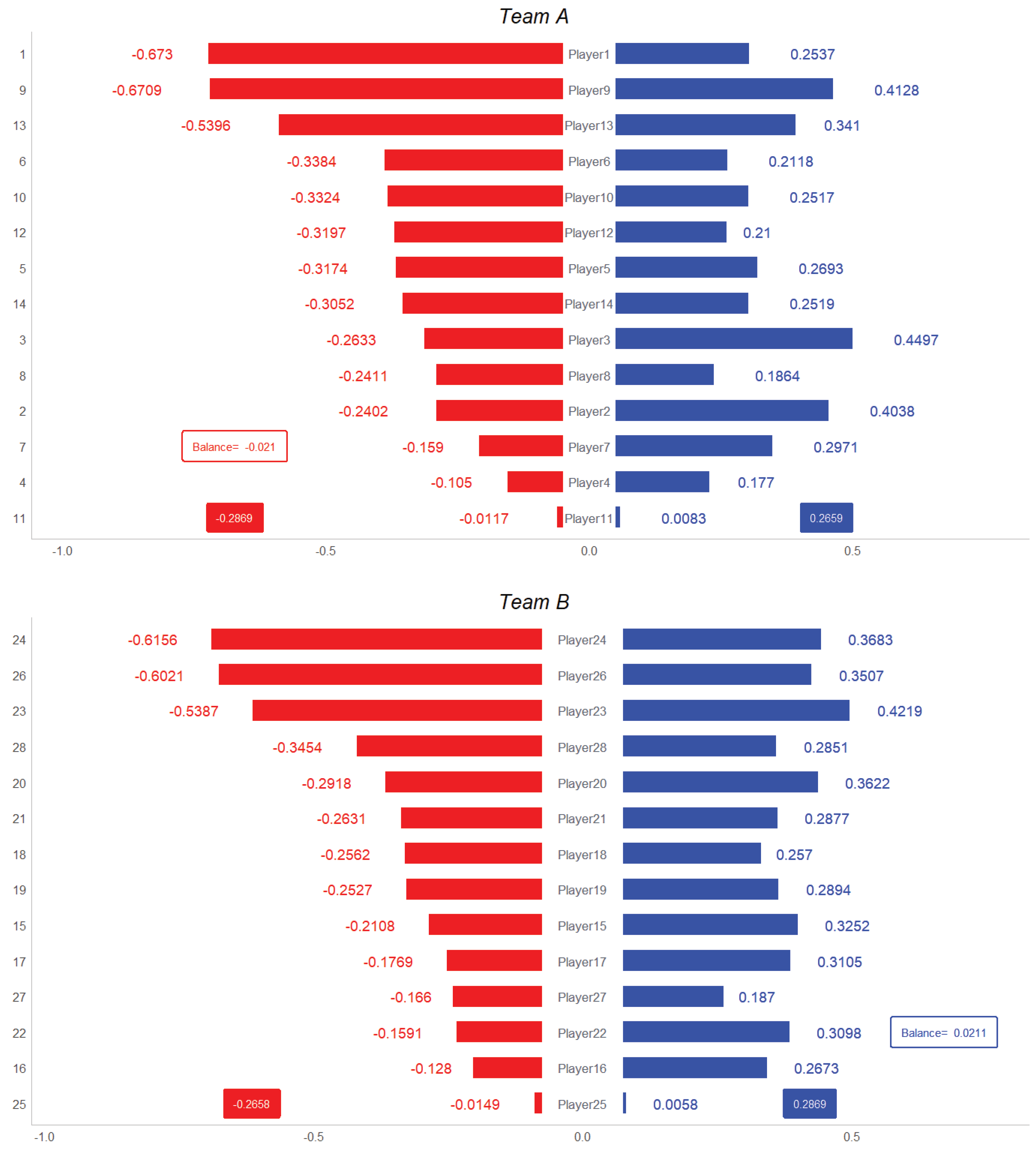
We finish with the efficiency of the pressure. As we said before not all the players play the same time. Hence we use the mean unitary pressure notion obtaining the mean defensive balance. This is shown in Figure 10. As we explain before here we use the mean unitary pressure, , as defined in (11) instead of .
During the match there were the following replacements:
• Team A: (1) ← (12), (6) ← (13), (10) ← (14).
• Team B: (22),(24) ← (26),(27), (19) ← (28).
Therefore comparing Figure 9 and Figure 10 we see that, for instance, player 3 from A team is now the player with more exerted pressure (with value ), but player 9 () is not longer the most defended player but this position has passed to player 1 (). With respect to team B, player 23 is still the player with the best pressure () but now closely followed by player 26 with value . This means that player 26 of B team has done a great deal of pressing during the time he has been on the pitch.
In addition, through Figure 9 and Figure 10 we can evaluate the goodness of the substitutions made in the match from the defensive point of view, that is, we observe that the unit pressures generated by player 12 () are lower than those of player 1 () which he has substituted but that of player 13 () has been much higher than that of player 6 () and that of player 14 () somewhat higher than those of player 10 () so that especially the substitution (6) ← (13) has been very productive for team A in terms of pressure generation.
4. Discussion
In football, the pressure exerted both between players and between teams is a very important tactical performance indicator and it comes fundamental to design game strategies, determining changes in players’ positions in the pitch, substitutions of players, spaces between lines...
Pressure evaluation is difficult because it is a metric that involves both individual players and groups of players. Therefore, having a simple and easily computable method to evaluate it from the data available in football can be useful for coaches and technical staffs.
In this paper we deal with a geometrical model of the definition of pressure. It starts from the elementary notion of area of influence, the area that is under the control of a player, which allows us to define the pressure exerted on a player based on the intersection of the areas of influence between the player who pressures and the player who is pressured. This distinction between the player exerting pressure and the player under pressure is made on the basis of which team is in possession of the ball at any given moment. This area of influence is established on the basis of a circumference centered on the player’s position with radius r. This radius, a unique value for the complete match, is determined via a compromise between in one hand a significant number of interactions N to allow accurate estimates and on the other hand avoiding to consider very distant players as participants in the pressure. We want to note that this is the only parameter of the model whose determination from the data is straightforward as explained in the SubSection 2.2.
An important advantage of our model is that, once the elementary amount of pressure between players is defined, with the same model and the same assumptions, it is very easy to obtain simultaneously pressure received by a player from the whole opponent team and also pressure exerted by a team on the whole opponent team, everything using the same dataset information on individual players. In particular, we can evaluate the goodness of the substitutions made in the match from the defensive perspective analysing the pressure exerted by the player and by the substitute. It is that we call the efficiency of the pressure.
Our pressure metrics (individual and collective) are defined frame by frame. Therefore they can also be extended to the whole duration of a football match, which implies that not only can give an static game perspective but also a time-dependent perspective on a given match. As future work we plan to explore this time dependence via this detailed frame-by-frame analysis.
We have performed an analysis of data from a real match showing the versatility of this metric. For doing that we have used tracking data with eventing that allows us to determine at each moment the position of each player in the pitch, i.e. their relative positions, as well as to know which team is in possession of the ball at each moment. In particular we have shown that in a simple way a global balance can be obtained between two teams over the course of a complete match. This analysis can be restricted to any time interval within the match, determining the balance of pressures at different instants of the game. The same analysis can be done on a player-by-player on the same conceptual basis.
In summary, the model presented here is mathematically simple, easily computable and flexible in that it supports player and team, static and dynamic time-dependent metrics and we believe it can be a useful tool for the tactical analysis of football matches by coaches and technical teams, as well as broadcasters and audiovisual media.
References
- O’Donoghue, P. The use of feedback videos in sport. International Journal of Performance Analysis in Sport 2006, 6, 1–14. [CrossRef]
- Mackenzie, R.; Cushion, C. Performance analysis in football: A critical review and implications for future research. Journal of Sports Sciences 2013, 31, 639–676. [CrossRef]
- Arnau Notari, A.R.; Calabuig, J.M.; Catalan, C.; Garcia-Raffi, L.M.; Pardo Gila, J.M.; Pons Anaya, R.; Sánchez Pérez, E.A. Using neural networks and hierarchical cluster analysis to study goal kicks in football. International Journal of Sports Science & Coaching 2023, 19, 17479541231207184, [https://doi.org/10.1177/17479541231207184]. [CrossRef]
- Smith, R.A.; Lyons, K. A strategic analysis of goals scored in open play in four fifa world cup football championships between 2002 and 2014. International Journal of Sports Science & Coaching 2017, 12, 398–403. [CrossRef]
- Taki, T.; Hasewaga, T.; Fukurama, T. Development of motion analysis system for quantitative evaluation of teamwork in soccer games. Proceedings of 3rd IEEE International Conference on Image Processing, 1996. [CrossRef]
- Hewitt, A.; Greenham, G.; Norton, K. Game style in soccer: what is it and can we quantify it? International Journal of Performance Analysis in Sport 2016, 16, 355–372. [CrossRef]
- Vidal-Codina, F.; Evans, N.; El Fakir, B.; Billingham, J. Automatic event detection in football using tracking data. Sports Engineering 2022, 25, 18. [CrossRef]
- Andrienko, G.; Andrienko, N.; Budziak, G.; Dykes, J.; Fuchs, G.; von Landesberger, T.; Weber, H. Visual analysis of pressure in football. Data Min Knowl Disc 2017, 31, 1793–1839. [CrossRef]
- Link, D.; Lang, S.; Seidenschwarz, P. Real time quantification of dangerousity in football using spatiotemporal tracking data. International Symposium on Computer Science in Sport 2019, pp. 1–16. [CrossRef]
- Memmert, D.; Raabe, D.; Schwab, S.; Rein, R. A tactical comparison of the 4-2-3-1 and 3-5-2 formation in soccer: A theory-oriented, experimental approach based on positional data in an 11 vs. 11 game set-up. PlosONE 2020. [CrossRef]
- Robberechts, P. Valuing the art of pressing. https://people.cs.kuleuven.be/~pieter.robberechts/repo/robberechts-statsbomb19-pressing.pdf, accessed on 2024.
- Forcher, L.; Forcher, L.; Altmann, S.; Jekauc, D.; Kempe, M. The keys of pressing to gain the ball – characteristics of defensive pressure in elite soccer using tracking data. Science and Medicine in Football 2022, pp. 1–9. [CrossRef]
- Metrica sports sample data. https://github.com/metrica-sports/sample-data, accessed on 2024.
Figure 1.
Influence area between players and depending on the radius r.
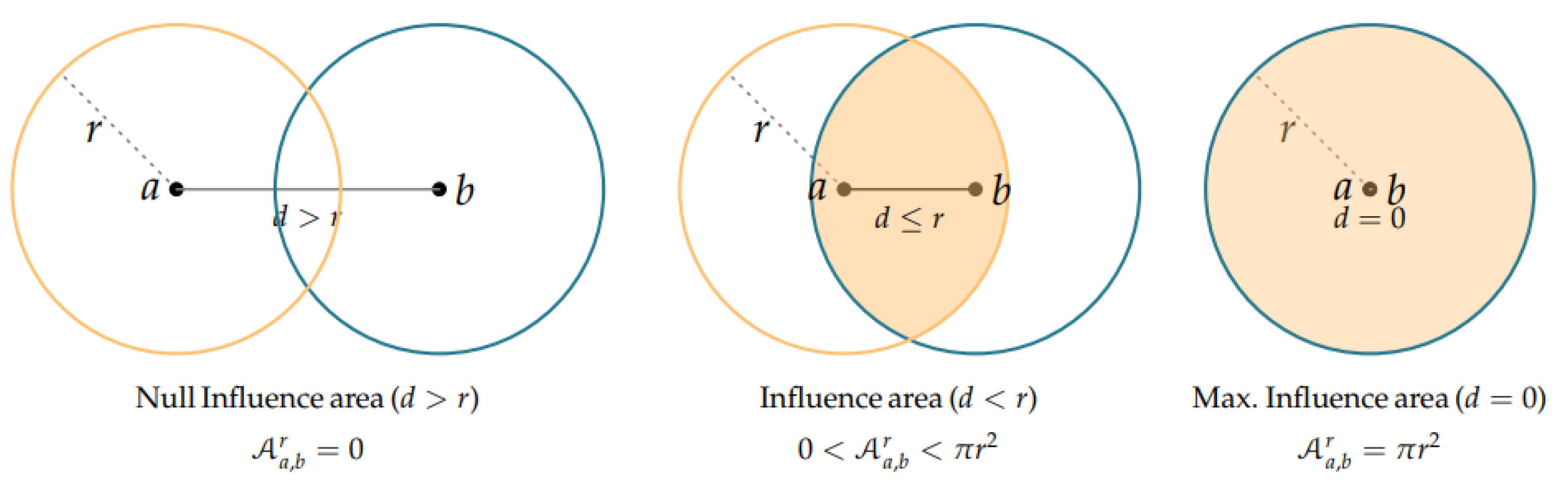
Figure 2.
Representation of the influence area function—left—and its approximations—right—for different ball sizes r— and —as a function of the distance .
Figure 2.
Representation of the influence area function—left—and its approximations—right—for different ball sizes r— and —as a function of the distance .
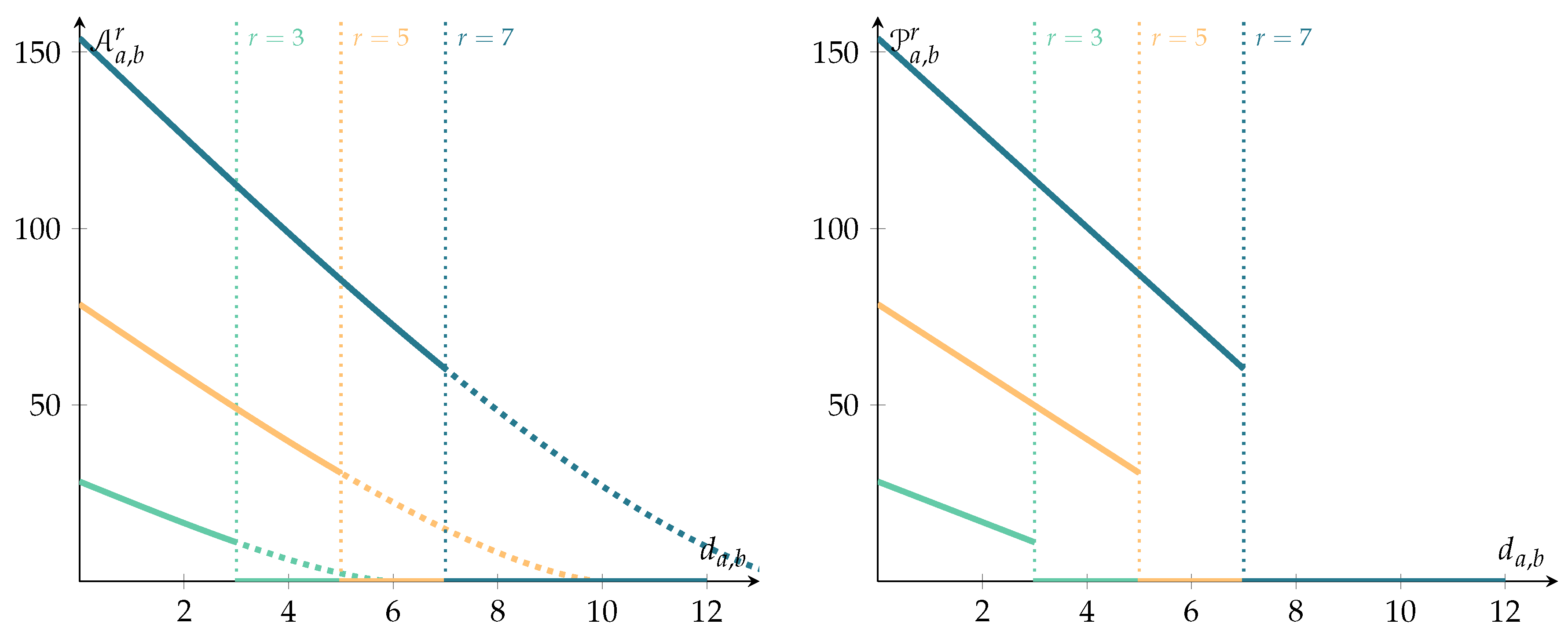
Figure 3.
Example of total number of pressure interactions between the two teams on a frame.
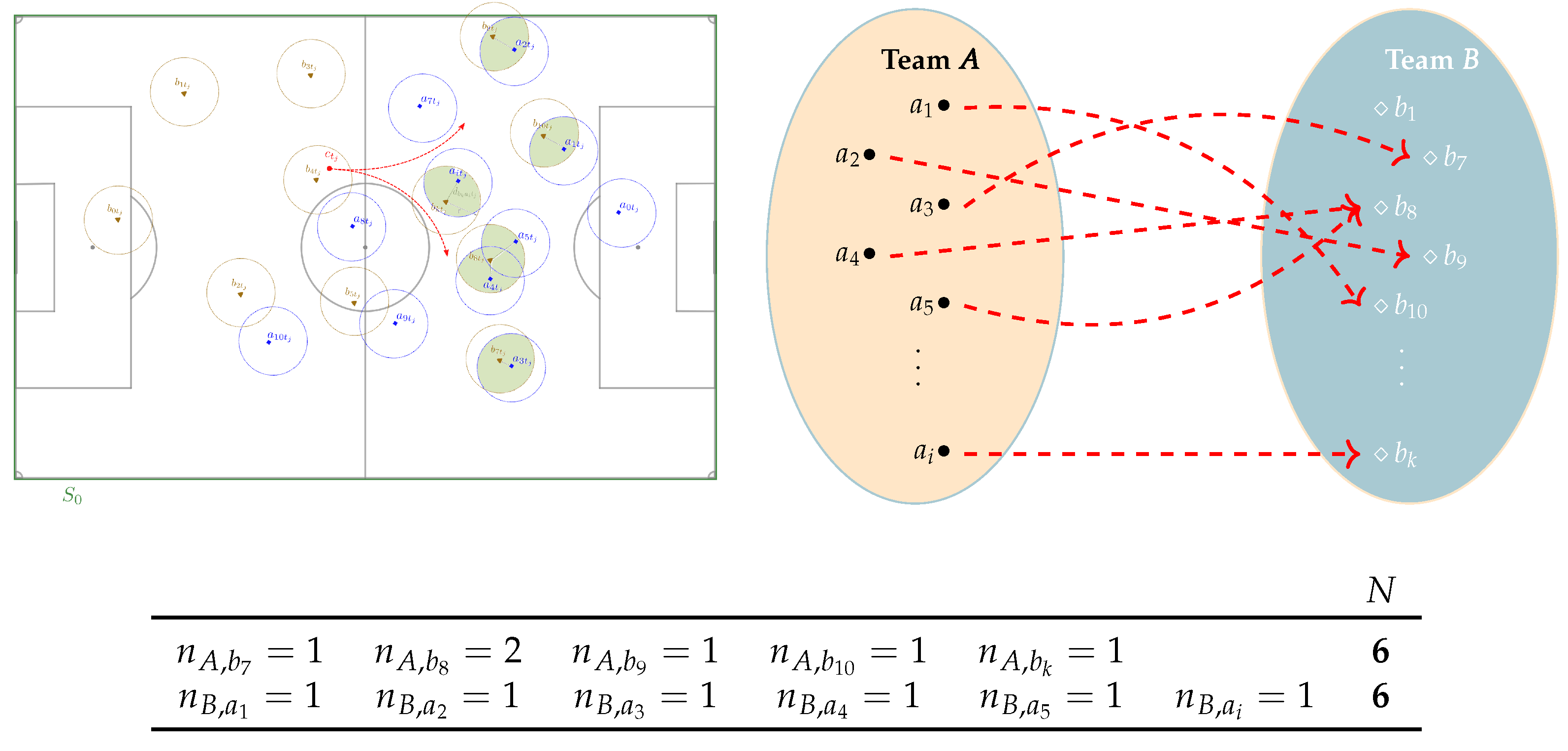
Figure 4.
sensibility to the ball radius variation in a frame .
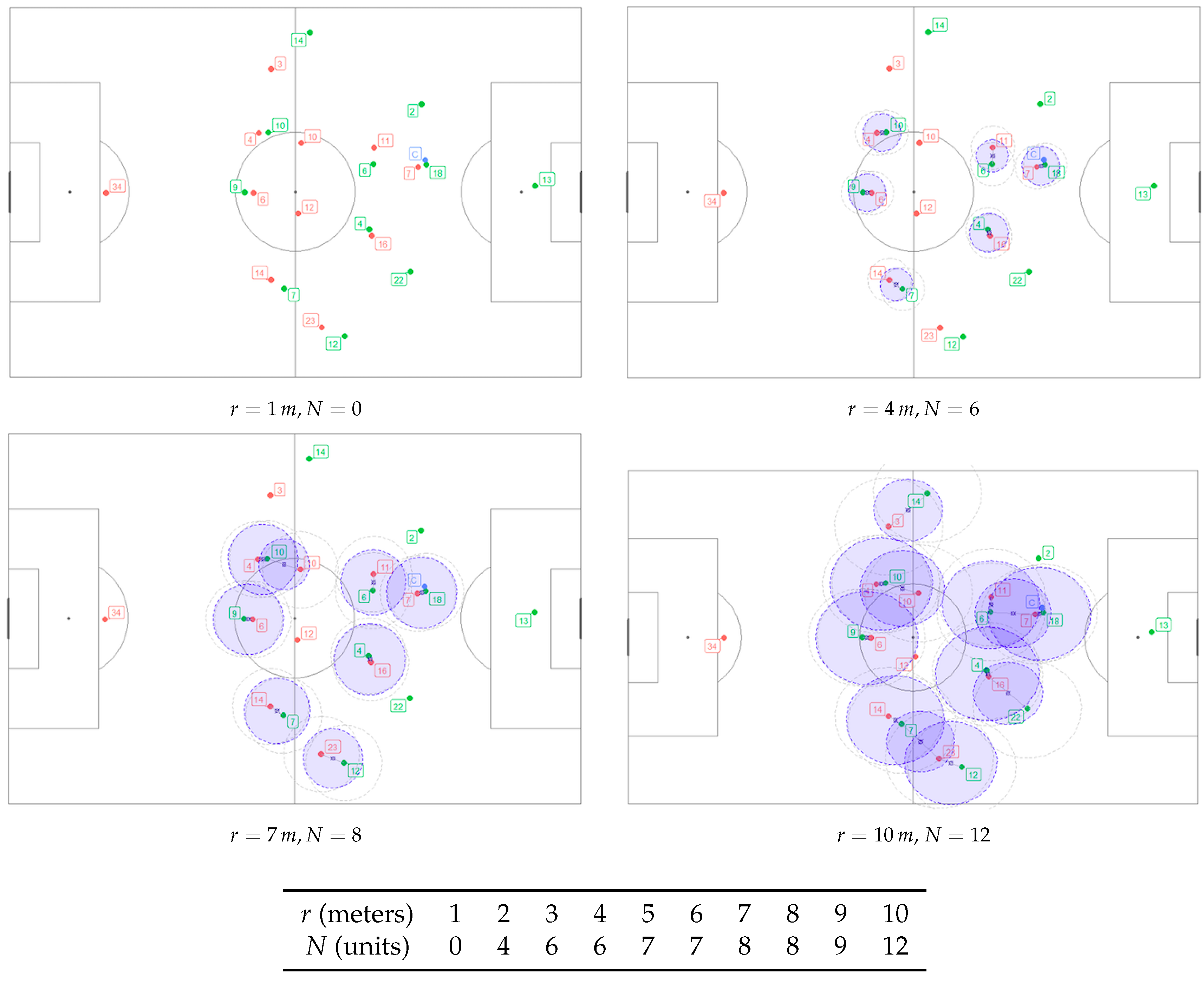
Figure 5.
Pressure distributions for different radii along the set of frames .
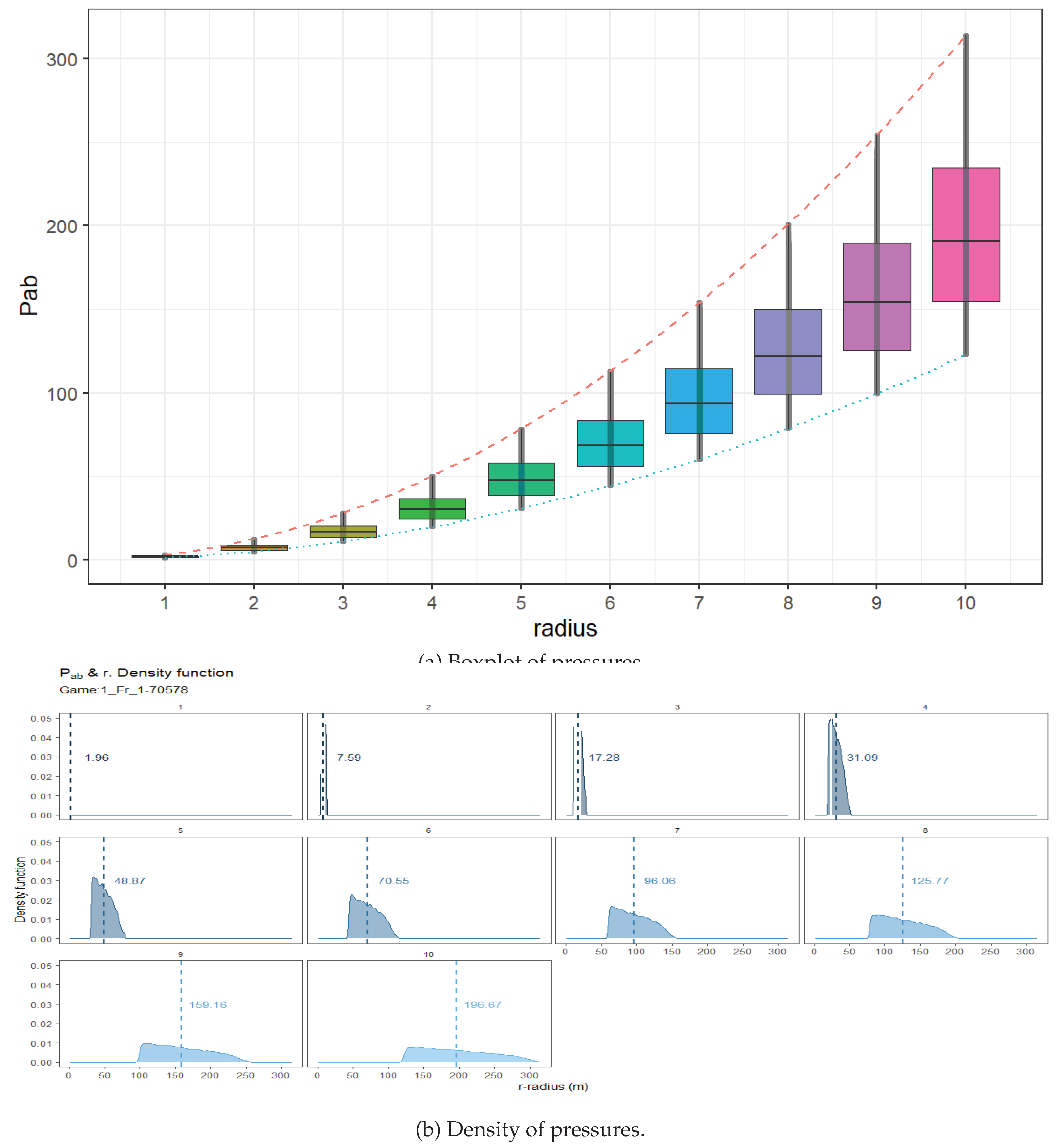
Figure 6.
Optimal ball radius using the normalized mean of the interactions and the normalized Curtosis of the number of interactions between players. We set the radius as meters.
Figure 6.
Optimal ball radius using the normalized mean of the interactions and the normalized Curtosis of the number of interactions between players. We set the radius as meters.
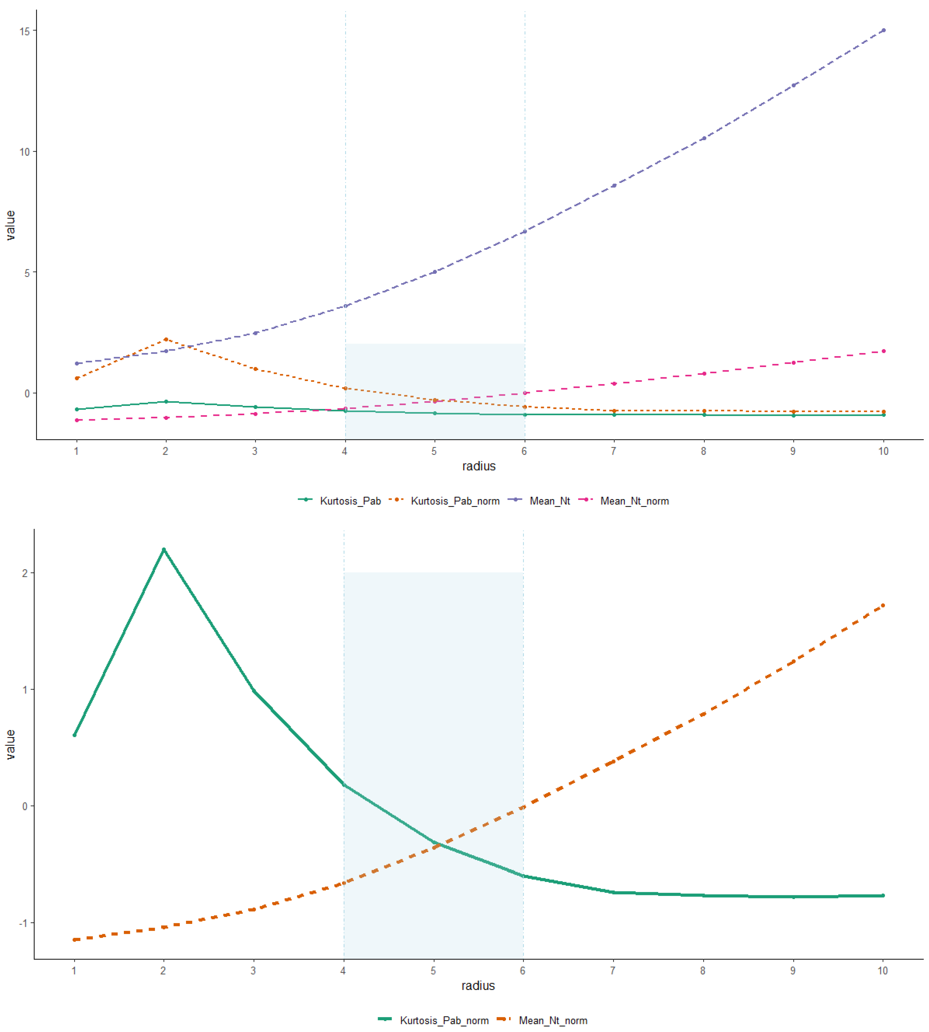
Figure 7.
Example of pressure with a set of three frames.
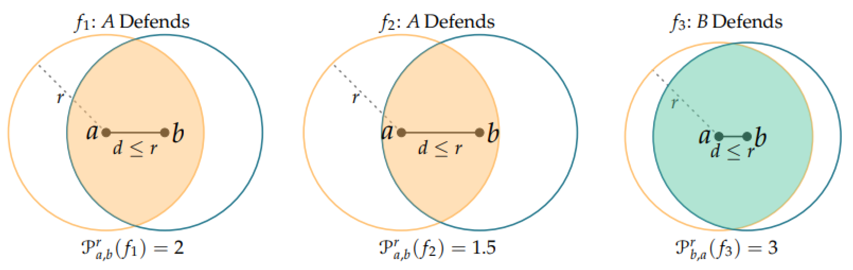
Figure 8.
Individual and collective pressure unitary metrics. Above: Exerted by team A and received by team B. Below: Exerted by team B and received by team B.
Figure 8.
Individual and collective pressure unitary metrics. Above: Exerted by team A and received by team B. Below: Exerted by team B and received by team B.
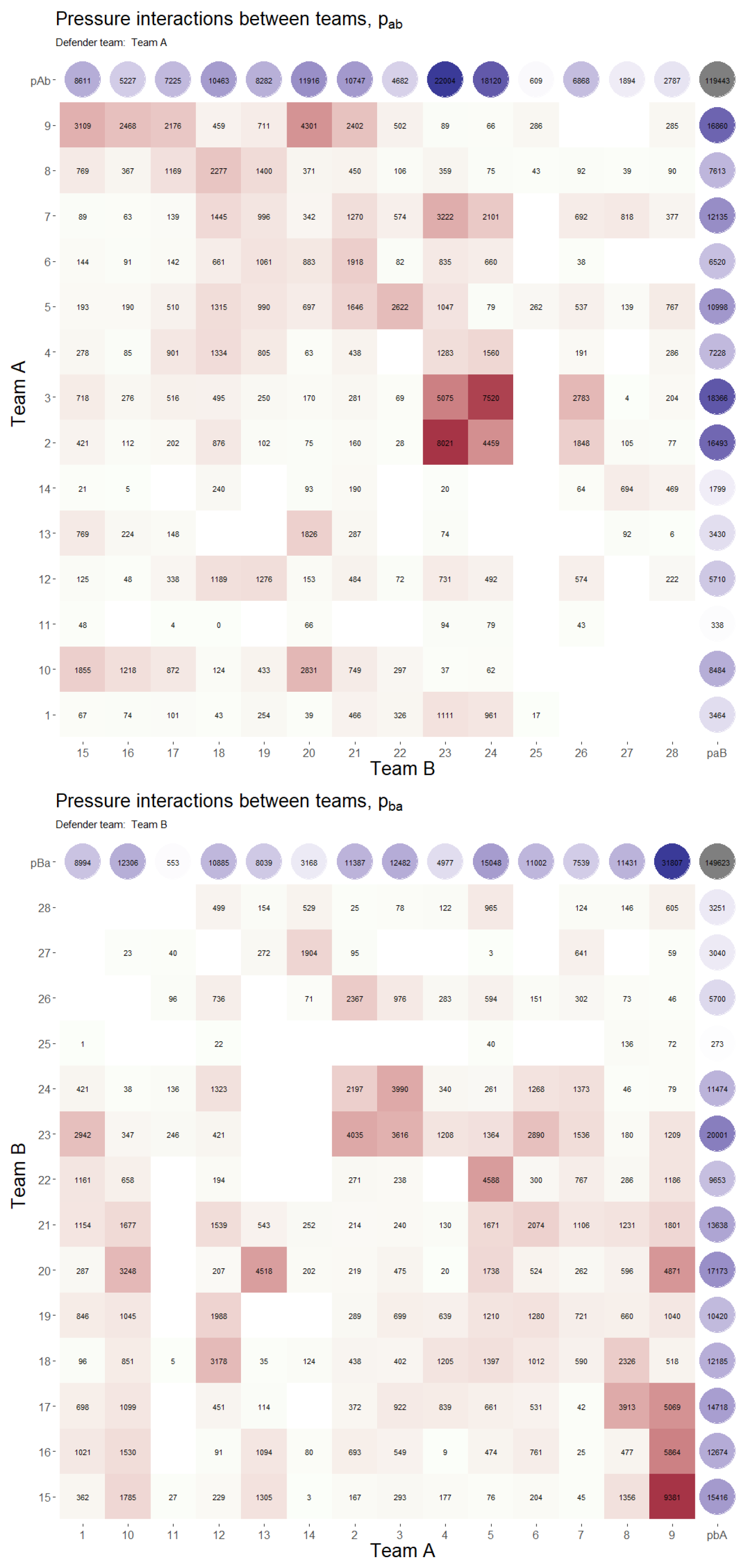
Figure 9.
Defensive balance obtained from the unitary pressure . Above: Team A players against B Team. Below: Team B players against A Team.
Figure 9.
Defensive balance obtained from the unitary pressure . Above: Team A players against B Team. Below: Team B players against A Team.
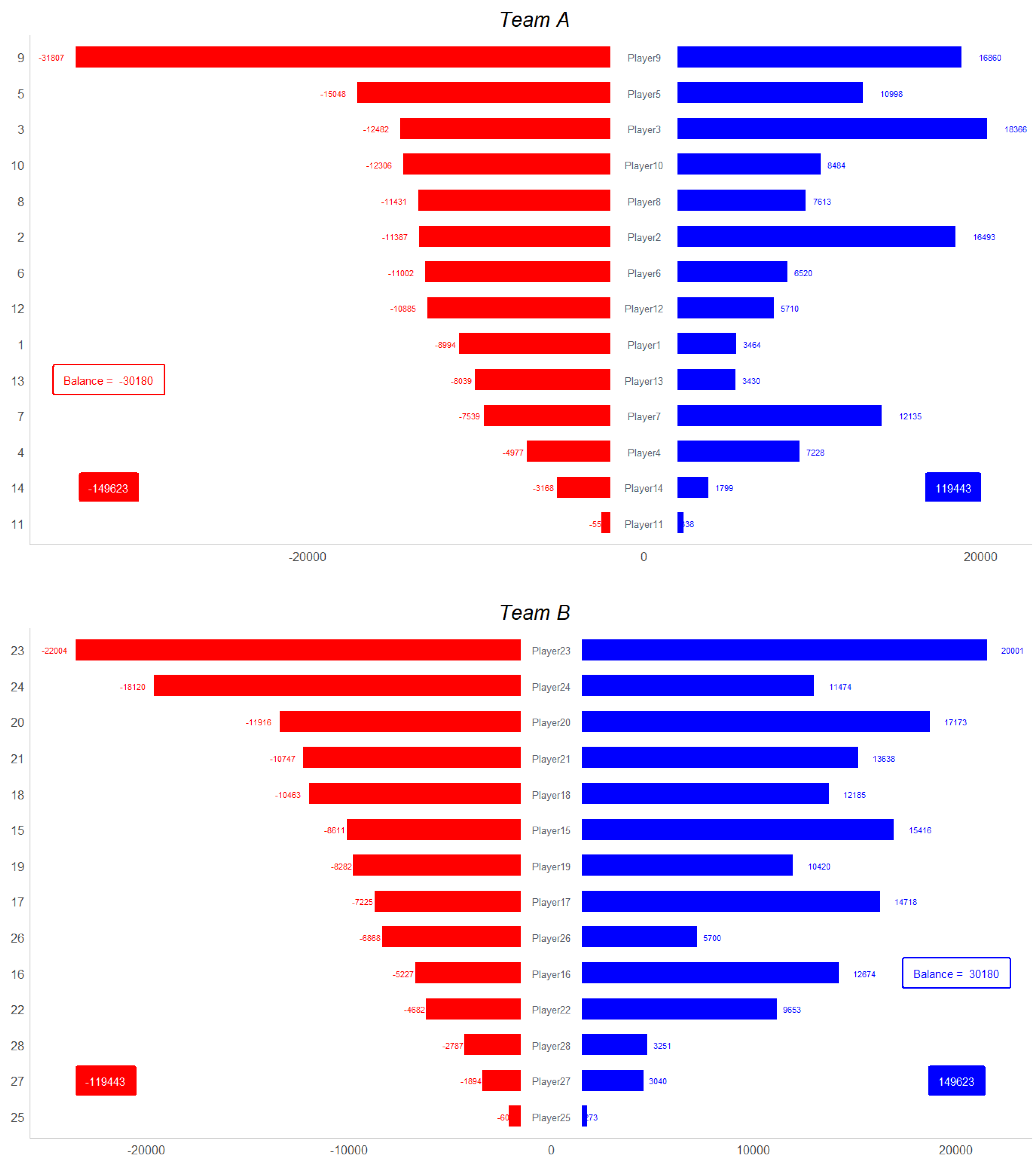
Figure 10.
Mean defensive balance obtained from the mean unitary pressure . Above: team A players against B team. Below: team B players against A team.
Figure 10.
Mean defensive balance obtained from the mean unitary pressure . Above: team A players against B team. Below: team B players against A team.
Disclaimer/Publisher’s Note: The statements, opinions and data contained in all publications are solely those of the individual author(s) and contributor(s) and not of MDPI and/or the editor(s). MDPI and/or the editor(s) disclaim responsibility for any injury to people or property resulting from any ideas, methods, instructions or products referred to in the content. |
© 2024 by the authors. Licensee MDPI, Basel, Switzerland. This article is an open access article distributed under the terms and conditions of the Creative Commons Attribution (CC BY) license (https://creativecommons.org/licenses/by/4.0/).
Copyright: This open access article is published under a Creative Commons CC BY 4.0 license, which permit the free download, distribution, and reuse, provided that the author and preprint are cited in any reuse.


