Submitted:
26 November 2024
Posted:
26 November 2024
You are already at the latest version
Abstract
This article presents the large-scale Integrated Scheduling Problem of TTC and DDT with Idle Degree Requirements (IS-TTC&DDT-IDR), which involves efficiently allocating antenna resources and scheduling tasks for tracking, telemetry, and command (TTC) as well as digital data transmission (DDT) in satellite ground stations. The problem aims to optimize task completion while managing idle resource capacity. To tackle this challenge, a Multi-Stages Local Search (MSLS) algorithm is proposed. The MSLS algorithm is designed based on the problem’s unique characteristics and is structured in three stages: the first stage uses a Forcibly Insertion Procedure (FIP) to generate a high-quality initial solution for DDT tasks, the second stage also uses the Forced Insertion Procedure (FIP) to optimize the TTC task, and the third stage enhances idle capacity through an Exchanging Procedure (EP). To design the experiments, this paper firstly extends task scale in quasi-real scenarios to ten-thousands level within a multi-satellite system, while current studies conduct their experiments in maximum 1600 tasks. Extensive empirical results based on such scenarios demonstrate that the MSLS algorithm outperforms reference algorithms on optimization value, stability, and convergence.
Keywords:
satellite scheduling
; multi-stage optimization
; integrated TTC and DDT scheduling
; heuristic methods
; local search algorithm
1. Introduction
Since artificial satellites possess a broad coverage, prolonged duration, and unique advantages unhindered by national borders or geographic constraints, they have been extensively employed across scientific exploration [1], economic development [2], as well as various military domains [3]. Because the limited autonomous ability of satellites, the tracking, measurement, control, and downlink of payload data of satellites heavily rely on the satellite ground stations [4]. Figure 1 illustrates the resource scheduling dilemma concerning satellite telemetry and control, as well as data transmission mission requirements. These operations related to the ground stations are mainly divided to two categories: Tracking, Telemetry, and Command (TTC) and Digital Data Transmission (DDT) tasks. With the increasingly number of satellite and user requirements, scheduling these tasks using limited antennas becomes a formidable challenge.
The TTC tasks scheduling problem involves the efficient allocation of antenna resources and scheduling of activities related to tracking, collecting telemetry data, and sending commands to spacecraft, satellites, or other aerospace vehicles [5]. This problem is a classical optimization problem and crucial for ensuring smooth operations, maintaining communication, and optimizing the use of resources in aerospace missions [6]. Generally, the objective of this problem can be maximizing resource utilization [7] and maximizing the task number [8] under satisfying a series of constraints. An effective plan involves allocating resources such as ground stations, antennas, communication links, and operating under real-time constraints [9]. The TTC tasks scheduling problem is a complex optimization challenge that requires careful planning, coordination, and decision-making to ensure the efficient and effective operation of aerospace missions. By addressing this problem effectively, aerospace organizations can enhance mission success, improve communication reliability, and optimize resource utilization in space exploration and satellite operations.
The DDT tasks scheduling problem involves the optimization of data transmission processes to ensure efficient and reliable communication between spacecraft, satellites, ground stations, and other components of the aerospace system [10]. This problem is crucial for managing the flow of data, minimizing transmission delays, optimizing bandwidth utilization, and ensuring the integrity of transmitted information [11]. Similar to the TTC tasks, this task should also should be completed by employing the resources related to the antennas and ground station. The objectives typically pertain to minimizing delay [12], maximizing data throughput [13], and guaranteeing data security [14]. At the same time, except the resource limitation, an effective plan should satisfy other constraints such as transmission deadlines, energy and electricity constraints. By effectively addressing the data transmission tasks scheduling problem, aerospace organizations can enhance communication efficiency, optimize data transmission processes, and ensure the timely and reliable exchange of information in aerospace missions. This contributes to improved mission performance, data integrity, and overall success in space exploration and satellite operations [10].
According to the similarity of these two scheduling problems, we observed that both the DDT and TTC tasks entail the utilization of ground stations and antennas. Consequently, formulating a unified strategy that encompasses both DDT and TTC tasks is feasible, as the combined issue necessitates antenna allocation. Since the Phased Array Antenna (PAA) is developed [15], this combined problem become possible. The PAA is a type of antenna system capable of controlling radiation direction by adjusting phase and amplitude, rendering it suitable for concurrent TTC and DDT [16]. Figure 1 displays distinct connections between antennas and satellites with the PAA. In this way, the DDT and TTC tasks can be executed simultaneously. Therefore, formulating an optimization model with decision variables associated with antennas is apt for addressing this issue. Moreover, as the number of satellites and antennas continues to rise, amalgamating dual task types undeniably amplifies the problem scale, thereby complicating the issue further. This truth brings higher demand for the scheduling strategy. Additionally, after reviewing the objectives of these two problem, we found that the objectives of these problems are normally designed for evaluating the effectiveness and resource utilization in a plan. And simply setting one objective is not sufficient to evaluate the merits of the entire plan.
According to the previous research, we propose a novel scheduling problem called the large-scale Integrated Scheduling Problem of TTC and DDT with Idle Degree Requirements (IS-TTC&DDT-IDR). This problem employs the antennas utilization as decision variables. Its objective is set as a score calculated by the sum of weighted one by the number of the completed tasks and the idle equipment. In this way, a novel objective is designed for assessing the effectiveness and resource utilization of a plan. Additionally, except usual constraints about TTC and DDT individually, within this scenario, there exists a discrepancy in antenna capabilities. The PAA can engage in both TTC and DDT simultaneously, whereas conventional antennas are confined to singular task functionalities. To solve this large-scale and complex optimization challenge, an effective algorithm is necessary.
Based on the unique attributes of this problem, we introduce an innovative algorithm termed the Multi-Stages Local Search (MSLS) algorithm. This method divides the optimization process into three distinct stages, with each stage dedicated to enhancing a specific objective through some effective operators, all the while guaranteeing the integrity of other potential profits. In the initial phase, the unscheduled DDT tasks are forcefully inserted into the scheduling plan, while the deleted tasks are reinserted by repair operator. This stage is made to maximize the number of completed DDT tasks. Transitioning to the second phase, the goal shifts to maximizing the completion tally of TTC tasks using analogous operators to those in the preceding stage. Notably, the scheduling plan is changed when the transmission process would not decrease the overall profits at this stage. And because the Visual Time Window (VTW) number of DDT is much less than that of TTC, prioritizing TTC scheduling initially tends to monopolize most resources, leaving scant room for DDT decisions. Thus, the sequence mandates DDT precedence over TTC. The last phase is dedicated to fine-tuning the idle capacity. Evidently, maximizing task fulfillment and idle resources pose conflicting objectives. Consequently, the primary two stages aim at task maximization without idleness constraints, whereas the last stage prioritizes enhancing the idle capacity. Here, as task removal from the high-quality scheduling plan could considerably dampen profit, we introduce a swapping operator to adjust the entire plan, ensuring the liberation of scheduling windows while safeguarding earning potentials.
In the experiments, we employ the data from Tianzhi Cup competition, which is collected from the real scheduling scenarios. Notably, the task number collected from 2-days or 4-days are ten thousands of levels. Thus, the experiments conducted by previous studies cannot match the current situation of the rapid increase in the number of satellites and task demand. To our best knowledge, the max task number from our study is 894137, which is largest scale in the current research and displays the most realistic representation of the current situation of the satellite management department. We conducted a series of comparative experiments, verifying the superiority of MSLS algorithm in objective values, stability, and iterative effectiveness. As a result, the MSLS algorithm reaches the maximum objective values in all real scenarios.
The contributions of this paper are follows:
- We introduce the IS-TTC&DDT-IDR problem, a large-scale Integrated Scheduling Problem for TTC and DDT tasks with Idle Degree Requirements. This problem involves efficiently allocating antenna resources and scheduling tasks for tracking, telemetry, and command (TTC) as well as digital data transmission (DDT) in satellite ground stations. To evaluate the effectiveness of our proposed model, we design and generate a set of 30 scenario instances of varying scales and complexities, all based on the large-scale telemetry tracking and control dataset provided by the Tianzhi Cup competition. The scenarios vary in terms of the number of antennas, satellites, total tasks, and available windows, providing a realistic benchmark for testing scheduling algorithms.For mirroring the real large-scale system, the largest scenario contains 50 antennas, 540 satellites, and totally 28544 tasks.
- We propose the MSLS algorithm, a novel approach for solving the integrated scheduling problem of DDT and TTC tasks. The algorithm divides the optimization process into three distinct phases, each with its own specific objective. In the first phase, the focus is on maximizing the completion of DDT tasks. The second phase targets the maximization of TTC task completion. Finally, the third phase is dedicated to increasing the degree of idleness, ensuring efficient resource utilization. This phased approach guarantees that each phase builds upon the solution of the previous phase, optimizing based on the outcomes of earlier stages while maintaining the independence of objectives. This ensures that the optimization in each phase improves upon prior results without causing negative impacts on the objectives achieved in earlier stages. Through this structure, our algorithm balances the competing demands of task completion and resource efficiency, offering a robust solution to the scheduling problem.
The remainder of this paper is structured as follows: Section 2 presents the related works about DDT and TTC tasks scheduling problem, and illustrate the motivation. Section 3 describe the IS-TTC&DDT-IDR problem and details its mathematical model. Section 4 introduce the MSLS algorithm in different stages and proposed operators. Section 5 presents comparative tests conducted on the real scheduling scenarios. Finally, Section 6 concludes the paper and discusses future research directions.
2. Related Works and Motivation
For solving the satellite task scheduling problem, many studies propose distinct algorithms. In addressing the DDT scheduling quandary, opting for a heuristic algorithm proves to be a sagacious decision. Zhang et al. [17] introduced an improved genetic algorithm, whose encoding and decoding is adopted to match the specific request with the corresponding satellite-ground resources. Additionally, the concept of a conflicting request set is put forth to confine the chromosome length, consequently diminishing the algorithmic time complexity. To navigate the delicate balance between diversity and convergence, a suite of potent operators is ushered in. These encompass population initialization structured around uniform design principles, multi-point greedy mutation, and adaptive selection procedures. This study amalgamates observation and data transmission tasks, showcasing the remarkable scalability of heuristic algorithms even as the optimization quandary grows in intricacy. Lin et al. [18] proposed a Sequential Two-Phased Heuristic Algorithm (STPHA). STPHA delineates an optimized Contract Plan (CP) using a Contract-Fast Construction Algorithm (CFCA) in its initial phase. Leveraging this CP as the foundation, it formulates an optimal transmission timetable through Linear Programming in its subsequent phase. The CFCA integrates an innovative heuristic named Mission Residual Volume Factor (MRVF), which steers the choice of suitable inter-satellite and satellite-to-ground links at each phase of construction. Similar to Lin’s study, Deng et al. [19] proposed a two-phase task scheduling algorithm. During the initial scheduling phase, a scheduling model is crafted with numerous constraint conditions, alongside an enhanced genetic algorithm featuring elite reservation tactics and a crowding function to uncover the initial scheduling solution. Transitioning to the dynamic scheduling phase, an exploration ensues into the potential for task preemptive switching and decomposition by formulating a dynamic scheduling model with diverse objectives: maximizing the total weight of scheduled tasks, minimizing alterations in the scheduling scheme, and reducing the count of decomposed sub-tasks. These studies illustrate the supremacy of segmenting the optimization procedure into distinct phases. In this way, a complex objective can be refined incrementally.
In TTC task scheduling problem, Liu et al. [20] introduced a constraint satisfaction problem alongside a local search algorithm designed to enhance scheduling efficiency. Their approach involves generating an initial foundational resource scheduling table guided by task priorities, subsequently allocating temporal TTC resources and addressing conflicts. They emphasize the efficacy of heuristic algorithms in augmenting search efficiency through the application of established rules and experiential knowledge to minimize the scope of exploration, rendering them well-suited for tackling expansive quandaries such as this. Nevertheless, the scale of their satellite study extends to only 19 units, while our current scope encompasses a significantly larger scale of 540 units. Bai et al. [21] proposed a multi-dimensional genetic encoding method to describe the problem. They meticulously outline the components of the algorithm, encompassing both the crossover and mutation operators, to construct a multi-dimensional Genetic Algorithm (GA) tailored for addressing the resource allocation problem. For improving the GA’s effectiveness on this problem, Chen et al. [22] proposed a population perturbation and elimination strategy based on GA (GA-PE). Initially, a task scheduling sequence is derived utilizing the GA-PE algorithm, followed by the application of a task planning algorithm to ascertain the schedulability of tasks. Comprehensive experiments examining strategy and parameter sensitivity verification have thoroughly probed the effectiveness of GA-PE across diverse facets. Li et al. [23] put forth two distinct serial structure hybrid methodologies that integrate single Ant Colony Optimization (ACO) with GA to address this particular problem. GA is employed to enhance the efficiency resulting from the initial stages of ACO, characterized by a scarcity of pheromone, and to avert premature convergence. These previous studies demonstrate that the TTC scheduling problem is complex with the huge decision space and constraints. Thus, the heuristic algorithms are effective to scheduling TTC tasks due to their high efficiency and scalability. Furthermore, embedded within a delineated optimization framework, these particular operators undeniably enhance the algorithm’s overarching efficacy.
Some other strategies are applied to the related scheduling problems. Wu et al. [24] introduced an amalgamation of metaheuristic and exact algorithms within a divide-and-conquer framework termed EHE-DCF, comprising a task allocation phase and a task scheduling phase. In the task allocation phase, individual tasks are assigned to appropriate orbits through a metaheuristic approach interwoven with probabilistic selection and a tabu procedure inspired by ant colony optimization and tabu search. Moving to the task scheduling phase, a task scheduling model is formulated for each distinct orbit and resolved utilizing a precise methodology, namely the branch and bound (B&B) technique. Wang et al. [25] presents an exact algorithm based on enumeration, in which each subproblem is solved by path programming, and all the feasible solutions of subproblems are combined to solve the master problem. Furthermore, three heuristics are designed to solve the large-scale problem due to the inefficacy of exact algorithms. While these methodologies have been utilized to achieve a promising solution in a large-scale scenarios, the largest scenario they address comprises only 1600 tasks, significantly less than the scope of our study in more than 20,000 tasks. Due to the complexity of this scheduling problem, the heuristic algorithm is more suitable and popular than the exact algorithms. Heuristic algorithms offer several advantages when applied to optimization problems, especially in situations where finding an exact solution is computationally infeasible or time-consuming.
Some studies propose deep reinforcement learning strategies to solve these associated problems. Ou et al. [26] introduced a sophisticated Deep Reinforcement Learning (DRL) approach, seamlessly integrated within a heuristic scheduling framework tailored for the intricate satellite range scheduling problem. The fundamental premise of this algorithm lies in the segmentation of the quandary into two distinct sub-problems: (1) The Assignment problem, entailing the allocation of individual tasks across various antennas, and (2) The Single antenna scheduling predicament, aimed at ascertaining the commencement and culmination timings for designated tasks on the antenna. Zhou et al. [27] initially conceptualize the online scheduling dilemma as an energy-limited Markov decision process (MDP). Subsequently, taking into account the dynamics of task arrivals, they introduce an innovative deep risk-sensitive reinforcement learning methodology. More precisely, the algorithm assesses risk – quantifying the energy consumption surpassing the limitation – for every state, and strives to identify the optimal parameter balancing the reduction of latency and risk, all the while acquiring knowledge of the most advantageous policy. Wen et al. [28] integrated scheduling data transmission and observation tasks and proposed a hybrid Actor-Critic reinforcement learning method. As a result, while this study yielded satisfactory outcomes in task completion, the extensive training time exceeding 2 hours per scenario indicates a substantial computational expense, further exacerbated by the comparatively modest scale of 500 tasks compared to our datasets. Based on these studies, because the DRL’s outstanding ability to handle high-dimensional data and sequential decision making offers a powerful framework for solving complex decision making problems, an increasingly number of studies propose related strategies to schedule the satellite tasks. Nonetheless, as the scenario scale escalates to the thousands, the intolerable prolongation of training time becomes apparent. With the task scale ranging from 3000 to 28544 in this study, the implementation of a DRL strategy proves to be unsuitable.
Obviously, employing the exact algorithm or DRL on a large-scale problem is infeasible while the largest task size is up to more than 20,000. Therefore, despite the application of exact algorithms and deep reinforcement learning strategies to address the satellite task scheduling problems, the heuristic algorithm emerges victorious. In this study, by combining two types of satellite tasks, the scale of the problem has increased dramatically in number of satellites, antennas, and tasks. Additionally, with the increasing number of constraints, this problem become more complicated. In pursuit of a viable solution swiftly, we opt for a local search framework as our primary approach, driven by its notable scalability and adaptability. The local search algorithm [29] is an optimization method that iteratively explore the neighborhood of a given solution to move towards better solutions within a search space. These algorithms start with an initial solution and make incremental changes to reach a local optimum. Examples of local search algorithms include Simulated Annealing [30] (SA), GA [31], and Tabu Search [32] (TS). Local search algorithms exhibit computational efficiency and rapid convergence towards optimal solutions, particularly within expansive and intricate search domains. They prove advantageous for scenarios where the sheer magnitude of the search space renders exact solutions unfeasible. These algorithms demonstrate robust scalability in addressing sizable scheduling quandaries laden with large-scale tasks, resources, and constraints. Furthermore, they adeptly tackle scheduling optimization challenges characterized by substantial complexity and variability. Noteworthy is their capacity to acclimatize to shifts in scheduling parameters or constraints, thereby accommodating modifications encompassing fresh prerequisites, priorities, or constraints with minimal alteration to the underlying algorithmic framework. Consequently, this algorithmic framework proves apt for addressing the IS-TTC&DDT-IDR problem, marked by its expansive scale, intricate constraints, and stringent efficacy and computational time imperatives.
Previous studies on satellite task scheduling problem have applied various heuristic algorithms within the local search framework to address task scheduling in satellite systems, often using multiple stages to refine different aspects of the scheduling problem. However, these existing algorithms have not thoroughly examined the specific challenges presented by the IS-TTC&DDT-IDR problem. The problem of satellite mission scheduling has been proved to be NP-hard in theory [33], and the IS-TTC&DDT-IDR is more complicated and difficult to solve because of its integrated scheduling and consideration of resource allocation. As a result, the existing algorithm fall short in addressing the unique complexities of this issue. To bridge this gap, we propose the MSLS algorithm, which introduces a three-phase approach to optimization. By leveraging innovative procedures such as forced insertion and exchange, our algorithm significantly enhances optimization efficiency, offering a tailored solution that meets the distinct requirements of the problem at hand.
3. Problem Description
The IS-TTC&DDT-IDR is an integrated large-scale problem of DDT and TTC task scheduling problem, requiring the task completion and idle degree simultaneously. This problem involves devising the execution strategy for antenna resources at each ground station, taking into account satellite measurement, control, data transmission requirements, and satellite application needs comprehensively. The aim of this strategic planning is to optimize the execution plan of mission demands within resource limits. In this problem, the visible arc segments of a satellite are determined by its orbital path and the location of the ground station. The scheduling center formulates scheduling plans based on specific task requirements, satellite visibility predictions, and mission attributes. Once the initial scheduling plan is outlined, it is communicated to the satellite and equipment. Upon receiving the scheduling plan, the satellite is required to execute mission demands according to the designated time segments and resource allocations. Simultaneously, ground station equipment must be configured and prepared in accordance with the scheduling plan to ensure the seamless fulfillment of mission requirements during satellite transits.
In practial situations, the visibility arc segments of a satellite are determined by its orbital path and ground station positioning. The scheduling center formulates resource scheduling plans based on specific task requirements, satellite visibility forecasts, and task attributes, including communication segments between the satellite and ground stations and the necessary equipment resources. The resource scheduling center must comprehensively consider satellite orbit parameters, ground station distribution, and other resource constraints to ensure the feasibility and effectiveness of the scheduling plan. Once an initial resource scheduling plan is established, it is communicated to the satellite and relevant equipment. The satellite is required to execute task according to the time segments and resource allocations, while ground station equipment must be appropriately configured and prepared based on the scheduling plan to ensure the smooth completion of task demands during satellite passes. This problem entails some specific optimization objectives along with a set of constraints, falling within the realm of optimization problems. However, due to the interdependency of its constraints and the high complexity stemming from the diversity of scenarios, precise solution algorithms and operations research algorithms may not yield acceptable effective solutions within a short timeframe. Hence, HAs and EAs are typically employed for resolution. Prior to the resolution process, data preprocessing is necessary, as well as the establishment of mathematical model for decision variables and constraint conditions. Subsequently, the design of specific operators and operational procedures during the iterative process of intelligent optimization is crucial, culminating in the derivation of efficient solutions.
The scenario data predominantly includes low orbit mission demand data, satellite orbit forecast data, equipment data, and various constraints. Mission demand data encompasses task identifiers, task task types (such as measurement and control task demands and data transmission task demands), beginning times, ending times, and the time segments within which task demands can be executed, defining the fundamental information and restrictions of each task demand. Satellite orbit forecast data pertains to visible arc segments for the satellite and equipment, comprising satellite identifiers, device identifiers, orbit cycle numbers, and orbital ascent or descent statuses, among other parameters. Device data involves equipment identifiers and periods of equipment unavailability, specifying which equipment can be used for task demands during specific time intervals. Moreover, constraints form a part of the input, covering unique allocation constraints for task demands, equipment availability constraints, equipment unavailability constraints, maximum elevation angle constraints, and constraints for different orbit cycles of task demands with the same satellite and type. These constraints ensure the rational allocation of task demands, conflict-free utilization of equipment, and satisfaction of conditions for task demand execution.
The problem result comprises the task scheduling plan, the task completion rate, and the idle degree. The scheduling plan utilizes binary variables to indicate whether a task is allocated to a specific device for execution during a particular time segment, reflecting the specific task allocation results. The task completion rate measures the overall completion status of DDT and TTC, aiming to maximize this ratio to enhance the effectiveness of task execution and resource utilization efficiency. The final output also includes information on equipment resource utilization and a task timetable, providing clear operational guidance for actual task demand execution and aiding in the analysis of the efficiency and optimization effects of the scheduling plan.
3.1. Mathematical Model
The parameters used in this model is following:
The decision variable equals 1 when the task is executed in ; otherwise, the value equals 0 when when the task is not executed in .
The problem objective is related to the task completion and idle degree, calculated as follows:
where denotes the weighted raio of idle degree to the objective; is the idle degree of a plan, calculated by the Equation 2:
Specifically, the Equation 2 displays the ratio of the total idle duration more than 10 seconds to the total idle duration. The idle duration more than 10s is considered as an effective idle timeslot, meaning any extra task can be scheduled in this timeslot.
The problem constraints are described as follows:
Equation 3 displays that any task can be executed by a window at most once.
Equation 4 displays the observation angle should be larger than the mininal angle of this VTW for any scheduled task.
Equation 7 and 8 require that any executed VTWs can not be overlapped if they belong the same antenna.
Figure 2 displays delineated forbidden period and tasks occupied period, while the remaining intervals represent the idle time resources of the antennas, marked in ➀, ➁, ➂, ➃ and ➄. Within these, the idle period exceeding 10 minutes are deemed as valid idle time, denoted as , which are the ➀, ➂, ➄.
3.2. Problem Challenges
For solving the IS-TTC&DDT-IDR problem, the proposed algorithm should overcome the following challenges:
- The requirements of DDT and TTC tasks often necessitate the utilization of the same satellite equipment, or at least partially overlapping components. However, due to resource constraints, there may be competition between these two types of task demands. For instance, during a specific time segment, a particular device may serve only one type of tasks. Thus, an effective algorithm should make a judicious allocation of these resources to avoid conflicts.
- The multiple constraints of this problem, such as unique task assignments, device forbidden periods, elevation angle requirements, must be collectively satisfied. The interplay among these constraints could render certain scheduling schemes unattainable, thereby confining the space of feasible solutions. When constructing the model, precise articulation and coordination of these constraints are essential to ensure the resolution process proceeds devoid of conflicts.
- As the number of task, devices, and visible arcs increases, the scale of the problem escalates rapidly, leading to a significant augmentation in computational complexity for resolution. Traditional algorithms may struggle to find the optimal solution within a reasonable timeframe, necessitating the consideration of designing efficient heuristic or metaheuristic algorithms for solving, in order to strike a balance between solution quality and resolution time.
4. Proposed Method
To solve the large-scale Integrated Scheduling Problem of TTC and DDT with Idle Degree Requirements (IS-TTC&DDT-IDR) problem, we propose a three-phase approach called Multi-Stages Local Search (MSLS) algorithm. This algorithm separates the optimization process into three stages according to the problem objectives. Since the objective of the IS-TTC&DDT-IDR is composed by the task completion and idle degree, our algorithm optimize each component at individual stage. For maximizing the task completion, we design the Forcily Insertion Procedure (FIP) for the first two stages. The DDT tasks are determined before TTC tasks because scheduling DDT task initially would not occupy much decision space affecting effectiveness of TTC tasks. The idle degree is optimized at the last stage with Exchanging procedure (EP). In this way, the objective is optimized comprehensively. The whole algorithm process is displayed in Figure 3.
From Figure 3, the first two phases are conducted both by the solution initialization and FIP. Phase one is dedicated to managing DDT tasks, whereas phase two is tailored for optimizing TTC tasks. Following the rough scheduling plan’s completion, phase three exclusively engages in EP to refine the plan without incurring any loss in profitability.
4.1. Algorithm Preprocessing
The preprocessing of the algorithm includes the filtering process of VTWs , the establishment of the conflict relationship between VTWs and the segmentation of VTWs. The filtering process means matching a list of support Windows for each task that meets its requirements (such as pitch Angle, lift rail, etc.). The establishment of conflict relationship is to determine the conflict relation of Windows in advance in order to avoid repeated constraint checking in the algorithm iteration process. And to mitigate the complexity of IS-TTC&DDT-IDR problem and treat all VTWs as equally capable of executing a single task, we segment the two types of VTWs on DDT/TTC and DDT&TTC antennas into two separate VTWs. Physical properties such as the start time and end time of the two split VTWs are identical. And the specific segmentation rules are as follows:
- For VTWs on DDT/TTC antennas, we establish a new VTW with identical attributes to the original VTW. The new VTW is designated for completing DDT tasks, while the original VTW is for TTC tasks. Both VTWs occupy the same amount of time on the same antenna, adhering to constraints that prohibit task overlap on the same antenna, ensuring they cannot be selected simultaneously.
- For DDT&TTC antennas, we create a new VTW with attributes mirroring the original VTW. Similar to the previous case, one VTW handles DDT tasks while the other manages TTC tasks. Despite both windows occupying the same amount of time on the same antenna, given that the antenna can be utilized concurrently for DDT and TTC tasks, it doesn’t violate the constraint of non-overlapping task arrangements on the same antenna, thus allowing them to be selected simultaneously.
After the window segmentation, the VTW conflicting list for a single window comprises all other windows on the same antenna that conflict in time occupation and all windows on the same track fulfilling the same task.
4.2. Solution Initialization
The IS-TTC&DDT-IDR problem exhibits a significant data scale and solution space. In order to enhance algorithm effectiveness and reduce solving time effectively, we introduced a greedy strategy tailored to this problem, aiming to secure an initial solution that yields greater returns. Notably, the solution initialization is made both in the phase one and two, which aim to obtain the inital solution for DDT and TTC tasks, respectively. Taking the phase one as an example, the pseudocode is displayed in Algorithm 1.
| Algorithm 1:Solution Initialization |
|
1.35
Require: Initial solution with unscheduled DDT task list ;
Ensure: The solution after solution construction of DDT scheduling phase;
while not all the task in the that has not been accessed do
Get the task which has not been accessed and has the lowest number of VTW; Get the VTW list for ; while not all the window in the has not been accessed do
Get the VTW has not been accessed and has the lowest number of conflict VTW; if can complete without conflict then
Select to complete for current solution
end if
end while
end whilereturn; |
In Algorithm 1, the line 2-3 continues to select the unscheduled tasks until the stop termination. The line 4-9 choose the optimal VTW for the selected task. The initialization of the solution involves maximizing task insertion to fully occupy entire VTWs.
4.3. Algorithm Operators
Before illustrating the optimization process, the applied algorithm operators in all stages are introduced in this section. These three operators are following described:
- Deletion Operator: Delet a scheduled task from the original solution. In this way, the occupied VTW becomes available. Additionally, if any task in the occupied VTW’s conflicting list has no conflicted VTW due to this operation, it also becomes available.
- Insertion Operator: Insert an unscheduled task into an available VTW based on the original solution. This operation can be made when any available VTW appears. Due to the absence of VTWs in the initial solution, this operation should be made after the deletion operator.
- Repair Operator: Repair an deleted task into an available VTW. This operation should be conducted after the deletion operator to prevent compromising the objective.
These three operators cooperate for achieving the FIP and EP at optimization phases.
4.4. Forcily Insertion Procedure
The FIP is conducted at the first two phases: the first phase is focused on maximizing the profitability of DDT tasks, while the second phase aims to optimize the profitability of TTC tasks.
An example process of FIP is displayed in Figure 4.
Based on Figure 4, the old solution is formulated according to the Algorithm 1. and are scheduled sequentially, but possesses no available VTW lastly. The deletion operator removes the from the in the old solution at the step 2. In this way, the becomes available. Furthermore, since the and are in the conflicting list of , the deletion operator also renders them available simultaneously. And then, the unscheduled tasks is inserted into the available VTW by the insertion operator. At the same time, since the and are both in the conflicting list of , they become conflicted. Fortunately, the is still available and it is visible to . Thus, the repair operator reinserts deleted task into the . Finally, , , and are all inserted into suitable VTWs with high task completion.
Due to the unique structural characteristics of the solution space under consideration, in order to circumvent the inefficacy of random perturbations in conventional algorithms, we have delineated a contiguous window list for an individual unselected window as its neighborhood structure, and have proffered deletion, insertion, and repair operators tailored to this neighborhood delineation for the efficient and expedient advancement of task completion rates.
Within FIP, the count of tasks inserted and those relinquished during the current operator is documented. If the number of tasks inserted surpasses those abandoned, the current solution is embraced. Conversely, if the number of task demands inserted is less than those relinquished, the current solution is denied.
If the current solution is not accepted, a rollback to the state before this attempt is initiated. In cases where the number of task demands inserted in the current attempt equals the number of tasks abandoned, acceptance of the current solution is determined by a specified probability. Should the solution not be accepted, a similar rollback to the state before this attempt is executed.
Algorithm 2 displays the FIP for the first two steps. The line 4-31 displays the all operators of the FIP. Specifically, line 14 signifies the deletion operator; line 17 denotes the insertion operator; and line 20 represents the repair operator.
| Algorithm 2:Forcily Insertion procedure Algorithm |
|
1.35
Require: Constructed Solution ;
Ensure: Improved Solution ;
while not meet the termination criterion do
record current solution as ; Randomly select a task ; if has not been finished then
Get the VTW list for ; while not all the has been visited do
Set the neighborhood set of ,
for , where is the conflicting VTW list for do
if is selected then
into the neighborhood VTW list of ; Get the finished task ; Get the VTW list of ; into the neighborhood VTW list of
set ,set , delete the task from the VTW
break; update the current solution ; set ,set , insert the task into the VTW ; for do
if If is selectable for unfinished task then
Set ,set
, update current solution; break; end if
end for
end if
end for
if if meet the acceptance criterion then
end if
end while
end if
end whilereturn; |
4.5. Exchanging Procedure
In the third stage of the algorithm, building upon the solutions achieved after the completion of the first two schedules, to enhance the idle resource ratio of antennas for an overall profit boost, we have devised a neighborhood structure for the selected windows. Subsequently, with respect to this neighborhood structure, an exchange operator has been introduced to elevate this metric. The EP is executed at the third phase, aiming to maximize the idle degree without harming the task completion by modifing the scheduling plan. Similar to the FIP, three operators collaborate successively to facilitate the two forms of exchange.
Two examples of EP display VTW exchanging and Task exchanging, respectively in Figure 4.
Based on Figure 5, the old solution is obtained according to the Algorithm 2. In VTW Exchange, the deletion operator removes the from , causing , , and are available due to the conflicting principle. The repair operator reinserts into another visual VTW . In other words, the VTW Exchange change the ’s scheduling VTW from to . In Task Exchange, after the deletion operator removes the from the VTW , the insertion operator inserts the unscheduled task into the visual and available VTW . In other words, the Task Exchange replace the scheduling task from to . Both EMs achieve more available VTW, rendering higher idle degree without hamring the original task completion.
| Algorithm 3:EP |
|
1.35
Require: Constructed Solution ;
Ensure: Improved Solution ;
while not meet the termination criterion do
record current solution as ; Randomly select a task ; if has been finished then
Get the selected VTW ; Set ; Get the VTW list for ; add into the neighborhood VTW list of ; Get the ; add into the neighborhood VTW list of
set , set , delete the task from the VTW
for do
if is selectable for unfinished task then
Set ,set
, update current solution; break; end if
end for
end if
if if meet the acceptance criterion then
end if
end whilereturn; |
Algorithm 3 displays the EP for the third stage. The line 2-19 represents the overall EP operations. Specifically, line 11 denotes the deletion operator; line 14 denotes the insertion or repair operator when the selected task is deleted or selected from the original solution.
5. Experiments
Past studies have only tested their algorithms on a small scale of scenarios, typically fewer than 20 satellites, with a limited number of tasks. This scale of data volume no longer meets current and future practical requirements, and is inadequate for testing the real performance of various algorithms. In order to more comprehensively assess and demonstrate the performance and efficiency of the MSLS algorithm, based on the large-scale telemetry tracking and control data set provided by the Tianzhi Cup competition, we have designed and generated 30 scenario instances of various scales and varying levels of complexity. All instances are named based on their scale, number of antennas, number of satellites, total number of tasks, and available windows. It should be noted that the scale of a scenario is not directly linked to its level of difficulty, but rather to the scheduling period, where S represents a two-days task schedule, M represents four-days, and L represents eight-days. The scenarios are scored such that completing all DDT tasks earns 200 points, completing all TTC tasks earns 100 points, and achieving a 100% idle resource ratio earns 200 points.
5.1. Experimental Settings
To comprehensively evaluate the performance of the MSLS algorithm, we introduced three representative comparison algorithms for telemetry tracking and control task scheduling problems: the Destruction-Repair algorithm (DR), Tabu Search algorithm (TS), and Adaptive Large Neighborhood Search algorithm (ALNS). Using the cplex solver was also considered, but even for the smallest data set, the cplex solver failed to give a solution in one day, so we only compared the results with the above three algorithms. To ensure fairness, all algorithms were implemented in C++ and executed in the same hardware environment, specifically an Intel(R) Core(TM) i9-12900H CPU running at a base frequency of 2.5GHz with a maximum turbo frequency of 5.0GHz.
In the experimental setup, the destruction level for the DR and ALNS was set at 1/10 of completed tasks, while the tabu list length for the TS algorithm was also set at 1/10 of completed tasks. To facilitate a comparative analysis within the same optimization cycle, the iteration time for all algorithms was uniformly set to 60 seconds. Specifically, the three comparison algorithms iterated for 60 seconds aiming to maximize their objective values, whereas the MSLS algorithm underwent the following three optimization phases within the same timeframe: 30 seconds for DDT optimization, 10 seconds for TTC optimization, and 20 seconds for idle resource ratio optimization.
Furthermore, all algorithms adopted identical heuristic rule for solution initialization, which has been given in Algotithm 1. This means that DR, TS and ALNS three comparison algorithms will have exactly the same initial solution benefit value, while MSLS will only get a lower initial solution benefit value because it only initializes DDT at the beginning. And the results of each algorithm were averaged over 10 runs to ensure the stability and reliability of the experimental outcomes.
5.2. Comparison with Other Methods
The comparison results of the four different algorithms across various scenarios have been summarized in Table 2, encompassing the completion rates for DDT, TTC, idle resource ratio, and the overall scores for each solution. For each comparison algorithm, "(+)," "(=)," and "(-)" respectively indicate whether the comparison algorithm outperformed/equaled/underperformed the MSLS algorithm on a specific metric. Additionally, a supplementary row at the bottom of Table 2 tallies the instances where each comparison algorithm outperformed/equaled/underperformed the MSLS algorithm across the 30 scenarios. The bolded values in the table represent the optimal value for each metric in every scenario.
5.2.1. Objective Values
From the Table 2, upon a thorough examination of the scores across various performance metrics, it is evident that, with the exception of specific scenarios where the TS algorithm outperforms the MSLS algorithm in terms of DDT completion rate, and certain cases where both the TS and DR algorithms match the MSLS algorithm in TTC completion rate, the MSLS algorithm consistently outperforms the other three comparison algorithms in all remaining metrics across every scenario tested. This pattern is particularly clear in the evaluation of resource idle rate. Notably, the MSLS algorithm demonstrates a significant advantage in the idle resource ratio, surpassing the performance of the other algorithms by a wide margin. This advantage in resource management is one of the primary factors that contribute to the MSLS algorithm securing the highest overall score across all 30 test scenarios.
Further analysis of the performance across different scenario scales reveals that the MSLS algorithm exhibits remarkable optimization capabilities, consistently maintaining high performance across three distinct scenario sizes. As the problem scale increases, the MSLS algorithm retains its efficiency, showcasing its adaptability and robustness in handling larger and more complex instances. In contrast, the Destruction-Repair (DR) and Adaptive Large Neighborhood Search (ALNS) algorithms exhibit a noticeable decline in optimization performance as the problem size grows, particularly in terms of task completion rate. While the MSLS algorithm remains resilient, the DR and ALNS algorithms struggle to maintain the same level of efficiency. Moreover, all three comparison algorithms experience a significant drop in their ability to optimize the idle resource ratio, with this deterioration becoming more pronounced as the scale of the scenario increases.
5.2.2. Algorithm Stability
In addition to the scoring metrics of the four algorithms, we also logged the performance results of the profit values for each algorithm across multiple runs in various scenarios. Based on this data, we generated box plots illustrating the distribution, central tendency, and outliers of the profit values for each algorithm across different scenarios. To better showcase the stability and other indicators of different algorithms at varying scenario scales, we have selected the box plots for the following scenarios for display: S_50_490_6464_206002, M_50_540_14272_454475, L_50_400_19840_684440, L_50_530_27968_894137. These box plots provide insight into the performance consistency and overall characteristics of the algorithms in these specific scenarios.
Figure 6, Figure 7, Figure 8 and Figure 9 display all objective values obtained by running four algorithms in 10 times in the selected scenarios. Compared to the other three comparison algorithms, MSLS demonstrates a smaller range in the box plots across various scenarios, particularly in large-scale scenarios. This indicates that the algorithm exhibits lower fluctuation and greater consistency in results compared to the other comparison algorithms. This highlights the robustness of MSLS, allowing for the stable provision of high-quality solutions, mitigating significant performance fluctuations due to changes in scenarios, and showcasing a broader applicability range.
5.2.3. Convergence Curve
To compare the convergence behavior among different algorithms, we have also selected iteration curve plots for the four algorithms in four different scenarios: S_50_490_6464_ 206002, M_50_540_14272_454475, L_50_400_19840_684440, L_50_530_27968_894137, showed in Figure 10 and Figure 11.
Upon examining the comparison between Figure 10 and Figure 11,it becomes evident that as the complexity of the scenarios increases, the search capabilities of the Destruction-Repair (DR) algorithm and the Adaptive Large Neighborhood Search (ALNS) algorithm experience a significant decline. This decline is attributed to the growing difficulty in navigating the solution space effectively as the number of variables and constraints escalate.
On the contrary, the Multi-Stages Local Search (MSLS) algorithm demonstrates remarkable resilience to increasing complexity. Although MSLS starts with comparatively lower profit values when pitted against the other three algorithms at the outset of the optimization process, it exhibits a consistent and steady improvement in its performance. This enhancement is primarily due to the strategic phase transitions and the dynamic switching of corresponding operators designed within the algorithm. The phase transitions allow MSLS to focus on different aspects of the problem sequentially, thereby optimizing the solution in a more targeted manner. The operator switches, on the other hand, enable the algorithm to adapt its approach based on the current state of the solution, facilitating a more efficient exploration of the solution space.
Moreover, during the critical TTC phase of the scheduling process, MSLS showcases its efficiency by successfully finalizing the entire schedule for TTC tasks. This achievement is particularly noteworthy as it accomplishes the task well within a significantly shorter timeframe than the maximum time limit of 10 seconds allocated for each phase. This rapid convergence highlights the effectiveness of MSLS in handling the urgent and time-sensitive nature of TTC tasks, ensuring that the scheduling remains feasible and responsive under stringent time constraints.
6. Conclusion
In this study, we introduced a novel problem IS-TTC&DDT-IDR considering DDT, TTC completion, and idle degree simultaneously, and proposed a multi-stage heuristic algorithm, the MSLS, specifically designed to address it. The MSLS employ the local search framework and separates iteration process in three stages. The comparative experiments in real scenarios reveal that the MSLS algorithm outperforms other algorithm in objective values, stability, iterative effectiveness.
In future research, we aim to develop more effective strategies for solving the IS-TTC&DDT-IDR problem. Exploring innovative methods for improving the quality of scheduling plan. Additionally, as the numbers of satellites and task rapidly increase, the computational time of this problem should be more important. Therefor, improving the algorithm’s runtime efficiency will be a crucial focus of our future work.
References
- Siddique, I. Small Satellites: Revolutionizing Space Exploration and Earth Observation. European Journal of Advances in Engineering and Technology 2024, 11, 118–124. [Google Scholar] [CrossRef]
- Klomp, J. Economic development and natural disasters: A satellite data analysis. Global Environmental Change 2016, 36, 67–88. [Google Scholar] [CrossRef]
- Routray, S.K.; Javali, A.; Sahoo, A.; Sharmila, K.; Anand, S. Military applications of satellite based IoT. In Proceedings of the 2020 Third International Conference on Smart Systems and Inventive Technology (ICSSIT). IEEE; 2020; pp. 122–127. [Google Scholar]
- Ukommi, U.; Ubom, E.; Ikpaya, I. Ground station design for satellite and space technology development. Am. J. Eng. Res 2022, 10, 12–19. [Google Scholar]
- Zhan, Y.; Wan, P.; Jiang, C.; Pan, X.; Chen, X.; Guo, S. Challenges and solutions for the satellite tracking, telemetry, and command system. IEEE Wireless Communications 2020, 27, 12–18. [Google Scholar] [CrossRef]
- Modenini, A.; Ripani, B. A tutorial on the tracking, telemetry, and command (TT&C) for space missions. IEEE Communications Surveys & Tutorials 2023, 25, 1510–1542. [Google Scholar]
- Zeng, G.; Zhan, Y.; Xie, H.; Jiang, C. Resource allocation for networked telemetry system of mega LEO satellite constellations. IEEE Transactions on Communications 2022, 70, 8215–8228. [Google Scholar] [CrossRef]
- Soma, P.; Venkateswarlu, S.; Santhalakshmi, S.; Bagchi, T.; Kumar, S. Multi-satellite scheduling using genetic algorithms. In Proceedings of the Space OPS 2004 conference; 2004; p. 515. [Google Scholar]
- Wang, W.; Zhang, Y.; Wang, X.; Xu, H.; Tian, H. Design of reconfigurable real-time telemetry monitoring and quantitative management system for remote sensing satellite in orbit. In Proceedings of the 2018 IEEE 3rd Advanced Information Technology, Electronic and Automation Control Conference (IAEAC). IEEE; 2018; pp. 1293–1297. [Google Scholar]
- Kodheli, O.; Lagunas, E.; Maturo, N.; Sharma, S.K.; Shankar, B.; Montoya, J.F.M.; Duncan, J.C.M.; Spano, D.; Chatzinotas, S.; Kisseleff, S.; et al. Satellite communications in the new space era: A survey and future challenges. IEEE Communications Surveys & Tutorials 2020, 23, 70–109. [Google Scholar]
- Prins, C. An overview of scheduling problems arising in satellite communications. Journal of the Operational Research Society 1994, 45, 611–623. [Google Scholar] [CrossRef]
- Chen, X.; Li, X.; Wang, X.; Luo, Q.; Wu, G. Task scheduling method for data relay satellite network considering breakpoint transmission. IEEE Transactions on Vehicular Technology 2020, 70, 844–857. [Google Scholar] [CrossRef]
- Li, J.; Wu, G.; Liao, T.; Fan, M.; Mao, X.; Pedrycz, W. Task scheduling under a novel framework for data relay satellite network via deep reinforcement learning. IEEE Transactions on Vehicular Technology 2023, 72, 6654–6668. [Google Scholar] [CrossRef]
- Lei, J.; Han, Z.; Vázquez-Castro, M.Á.; Hjorungnes, A. Secure satellite communication systems design with individual secrecy rate constraints. IEEE Transactions on Information Forensics and Security 2011, 6, 661–671. [Google Scholar] [CrossRef]
- Mailloux, R.J. Phased array antenna handbook; Artech house, 2017.
- Gao, S.; Rahmat-Samii, Y.; Hodges, R.E.; Yang, X.X. Advanced antennas for small satellites. Proceedings of the IEEE 2018, 106, 391–403. [Google Scholar] [CrossRef]
- Zhang, J.; Xing, L. An improved genetic algorithm for the integrated satellite imaging and data transmission scheduling problem. Computers & Operations Research 2022, 139, 105626. [Google Scholar]
- Lin, X.; Chen, Y.; Xue, J.; Zhang, B.; He, L.; Chen, Y. Large-volume LEO satellite imaging data networked transmission scheduling problem: Model and algorithm. Expert Systems with Applications 2024, 249, 123649. [Google Scholar] [CrossRef]
- Deng, B.; Jiang, C.; Kuang, L.; Guo, S.; Lu, J.; Zhao, S. Two-phase task scheduling in data relay satellite systems. IEEE Transactions on Vehicular Technology 2017, 67, 1782–1793. [Google Scholar] [CrossRef]
- Liu, J.p.; Li, J.; Bai, J.; Yu, P.j. A Heuristic Algorithm of Space-Ground Cooperative TT&C Resources Scheduling. In Proceedings of the 2010 International Conference on Artificial Intelligence and Computational Intelligence. IEEE, Vol. 2; 2010; pp. 425–428. [Google Scholar]
- Bai, J.; Gao, H.; Gu, X.; Yang, H. A multi-dimensional genetic algorithm for spacecraft TT&C resources unified scheduling. In Proceedings of the Proceedings of the 28th Conference of Spacecraft TT& C Technology in China: Openness, Integration and Intelligent Interconnection 28. Springer, 2018; pp. 153–163. [Google Scholar]
- Chen, M.; Wen, J.; Song, Y.J.; Xing, L.n.; Chen, Y.w. A population perturbation and elimination strategy based genetic algorithm for multi-satellite TT&C scheduling problem. Swarm and Evolutionary Computation 2021, 65, 100912. [Google Scholar]
- Li, Z.; Li, J.; Mu, W. Space-ground TT&C resources integrated scheduling based on the hybrid ant colony optimization. In Proceedings of the Proceedings of the 28th Conference of Spacecraft TT& C Technology in China: Openness, Integration and Intelligent Interconnection 28. Springer, 2018; pp. 179–196. [Google Scholar]
- Wu, G.; Luo, Q.; Du, X.; Chen, Y.; Suganthan, P.N.; Wang, X. Ensemble of metaheuristic and exact algorithm based on the divide-and-conquer framework for multisatellite observation scheduling. IEEE Transactions on Aerospace and Electronic Systems 2022, 58, 4396–4408. [Google Scholar] [CrossRef]
- Wang, J.; Demeulemeester, E.; Hu, X.; Qiu, D.; Liu, J. Exact and heuristic scheduling algorithms for multiple earth observation satellites under uncertainties of clouds. IEEE Systems Journal 2018, 13, 3556–3567. [Google Scholar] [CrossRef]
- Ou, J.; Xing, L.; Yao, F.; Li, M.; Lv, J.; He, Y.; Song, Y.; Wu, J.; Zhang, G. Deep reinforcement learning method for satellite range scheduling problem. Swarm and Evolutionary Computation 2023, 77, 101233. [Google Scholar] [CrossRef]
- Zhou, C.; Wu, W.; He, H.; Yang, P.; Lyu, F.; Cheng, N.; Shen, X. Deep reinforcement learning for delay-oriented IoT task scheduling in SAGIN. IEEE Transactions on Wireless Communications 2020, 20, 911–925. [Google Scholar] [CrossRef]
- Wen, Z.; Li, L.; Song, J.; Zhang, S.; Hu, H. Scheduling single-satellite observation and transmission tasks by using hybrid Actor-Critic reinforcement learning. Advances in Space Research 2023, 71, 3883–3896. [Google Scholar] [CrossRef]
- Lourenço, H.R.; Martin, O.C.; Stützle, T. Iterated local search. In Handbook of metaheuristics; Springer, 2003; pp. 320–353.
- Bertsimas, D.; Tsitsiklis, J. Simulated annealing. Statistical science 1993, 8, 10–15. [Google Scholar] [CrossRef]
- Mirjalili, S.; Mirjalili, S. Genetic algorithm. Evolutionary algorithms and neural networks: theory and applications.
- Gendreau, M. An introduction to tabu search. In Handbook of metaheuristics; Springer, 2003; pp. 37–54.
- Vazquez, A.J.; Erwin, R.S. On the tractability of satellite range scheduling. Optimization Letters 2015, 9, 311–327. [Google Scholar] [CrossRef]
Figure 1.
Different connections between antennas and satellites.
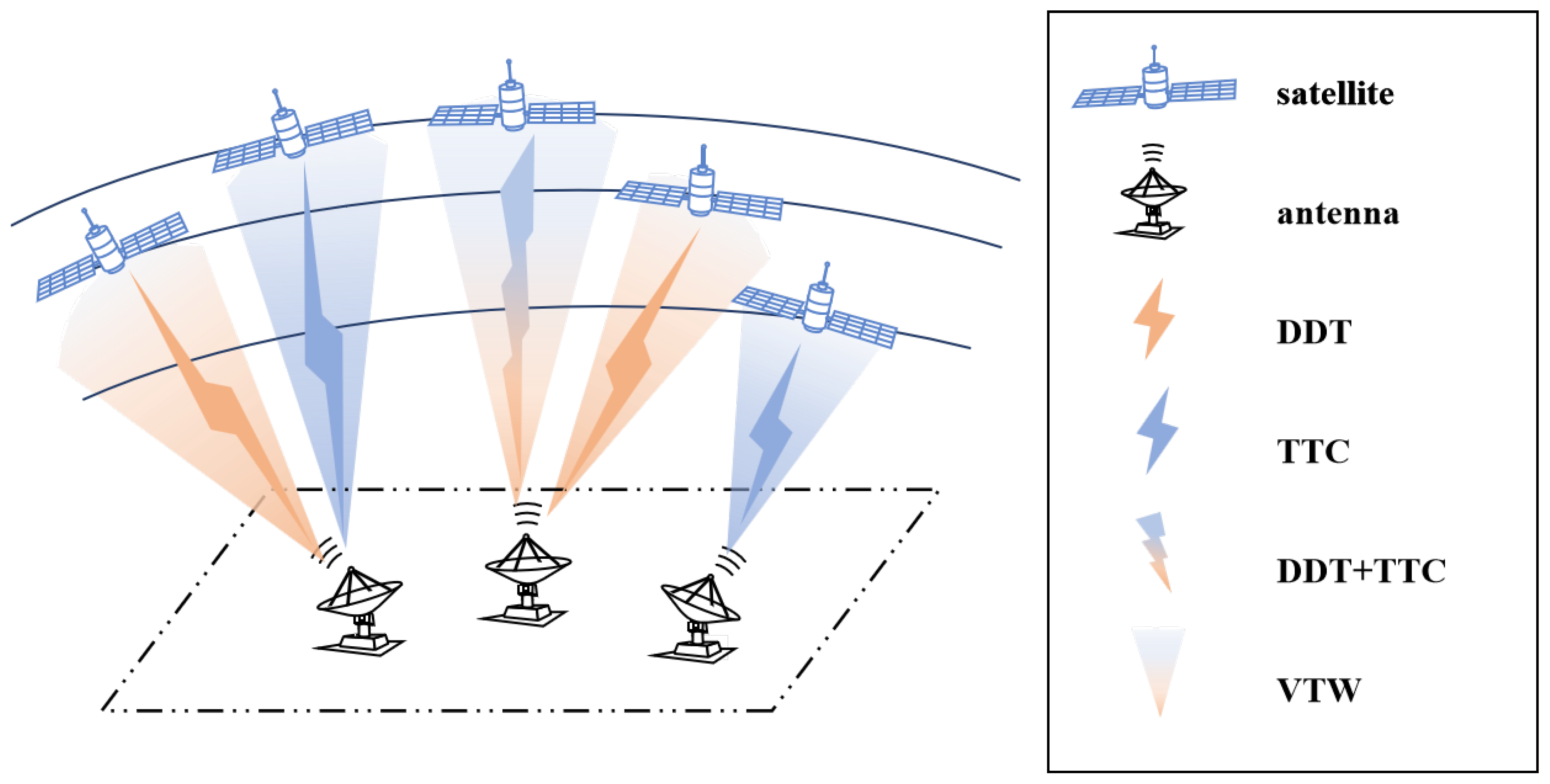
Figure 2.
The relationship among the idle period, forbidden period, and tasks occupied period.
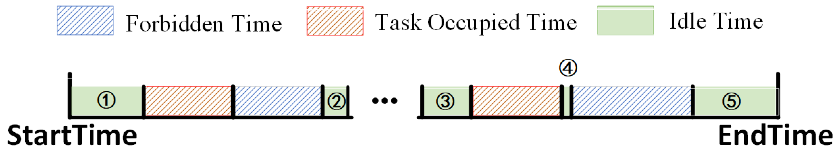
Figure 3.
The Algorithm Process. After the algorithm preprocessing, we carry out DDT scheduling, TTC scheduling and idle rate scheduling in turn.
Figure 3.
The Algorithm Process. After the algorithm preprocessing, we carry out DDT scheduling, TTC scheduling and idle rate scheduling in turn.
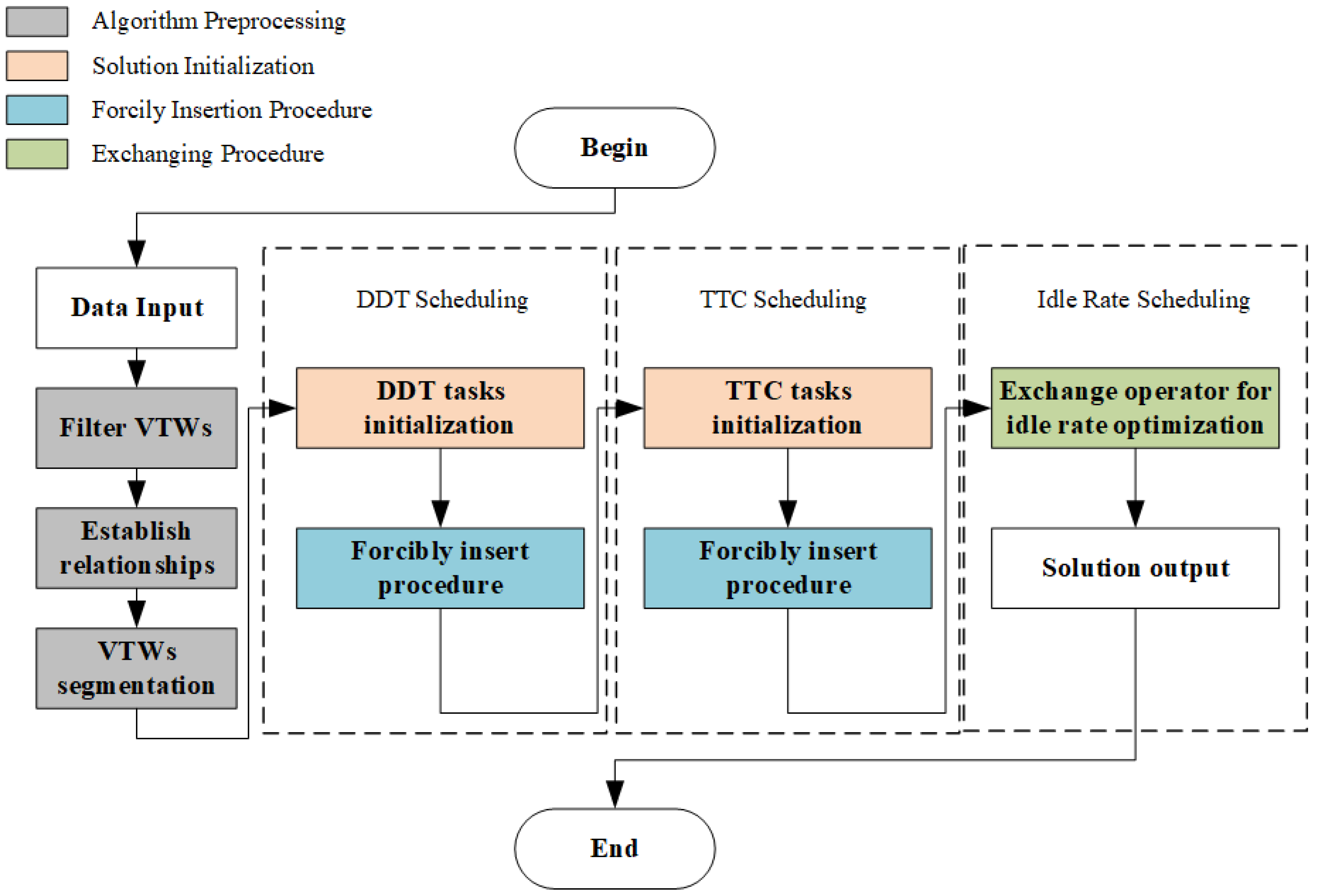
Figure 4.
The Forcily Insertion Procedure. The box in different color indicates the VTW under distinct condition; VTW Lists display the VTWs for each task; Conflicting Lists display the conflicting tasks corresponding to each task; Three operators cooperate in sequence for completing the FIP.
Figure 4.
The Forcily Insertion Procedure. The box in different color indicates the VTW under distinct condition; VTW Lists display the VTWs for each task; Conflicting Lists display the conflicting tasks corresponding to each task; Three operators cooperate in sequence for completing the FIP.
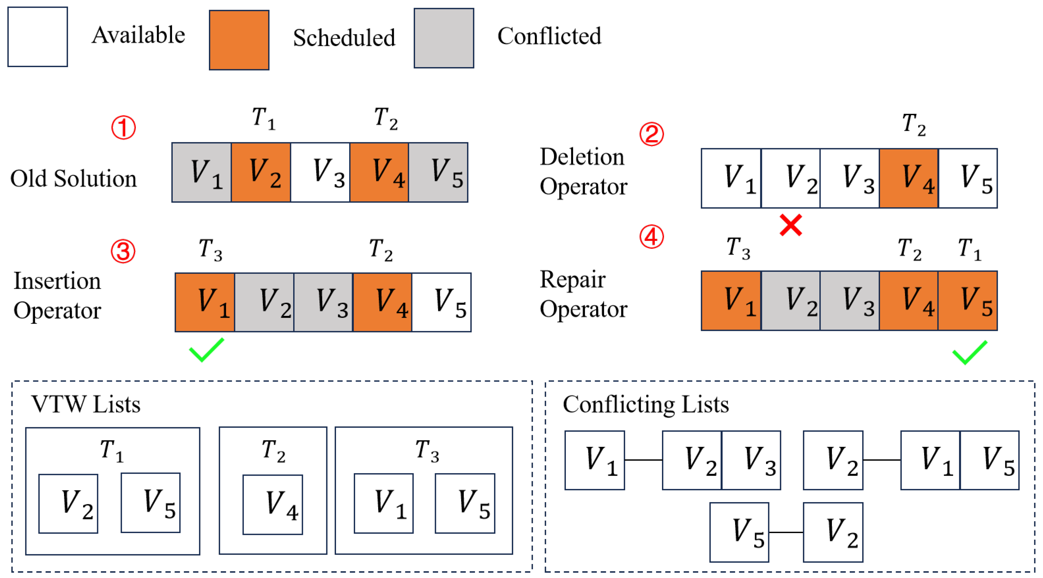
Figure 5.
The Exchanging Procedure. The box in different color indicates the VTW under distinct condition; VTW Lists display the VTWs for each task; Conflicting Lists display the conflicting tasks corresponding to each task; Three operators cooperate in sequence for completing the EP in two forms.
Figure 5.
The Exchanging Procedure. The box in different color indicates the VTW under distinct condition; VTW Lists display the VTWs for each task; Conflicting Lists display the conflicting tasks corresponding to each task; Three operators cooperate in sequence for completing the EP in two forms.
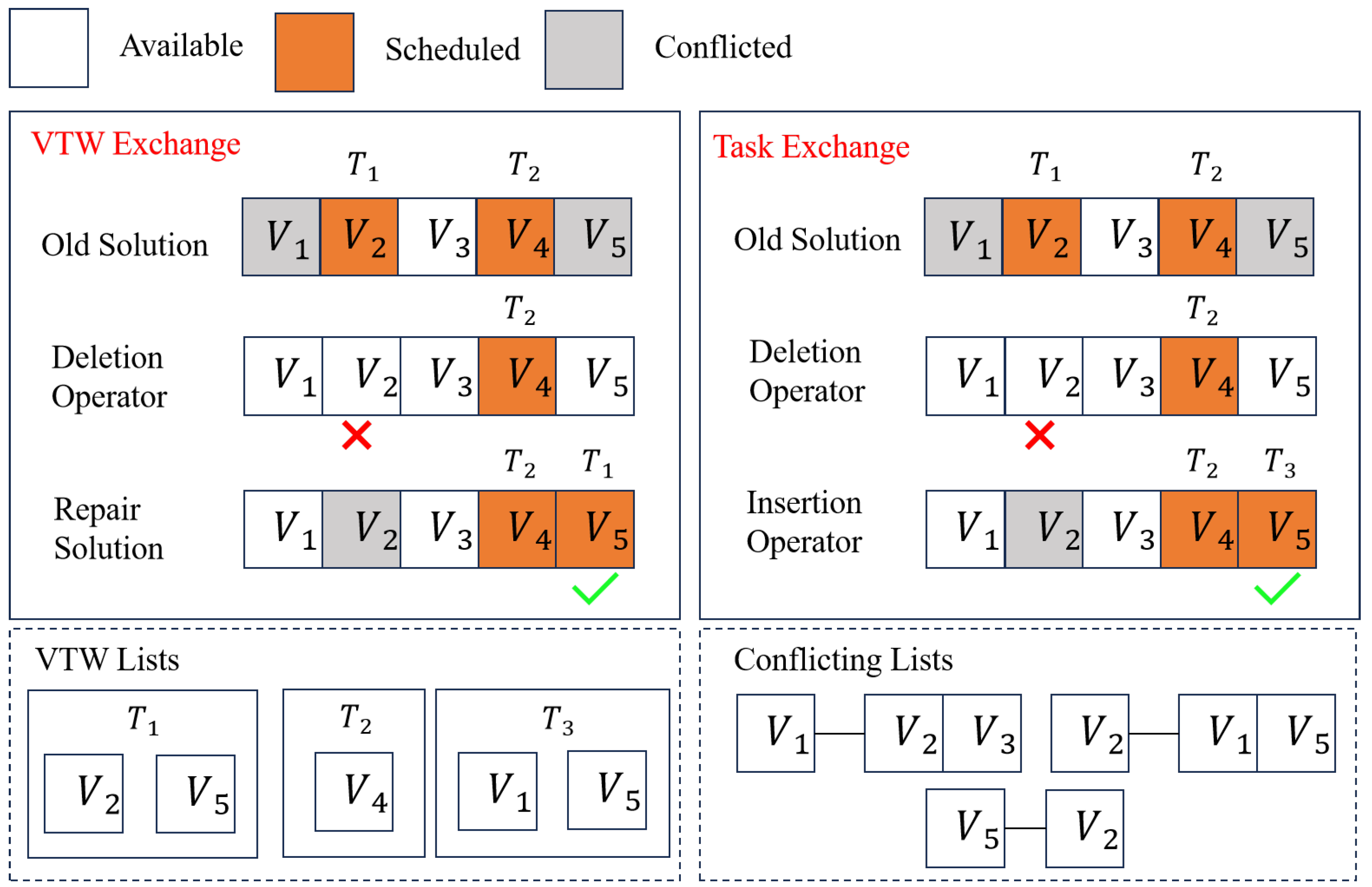
Figure 6.
Objective values obtained by running four algorithms 10 times in scenario S_50_490_6464_206002.
Figure 6.
Objective values obtained by running four algorithms 10 times in scenario S_50_490_6464_206002.
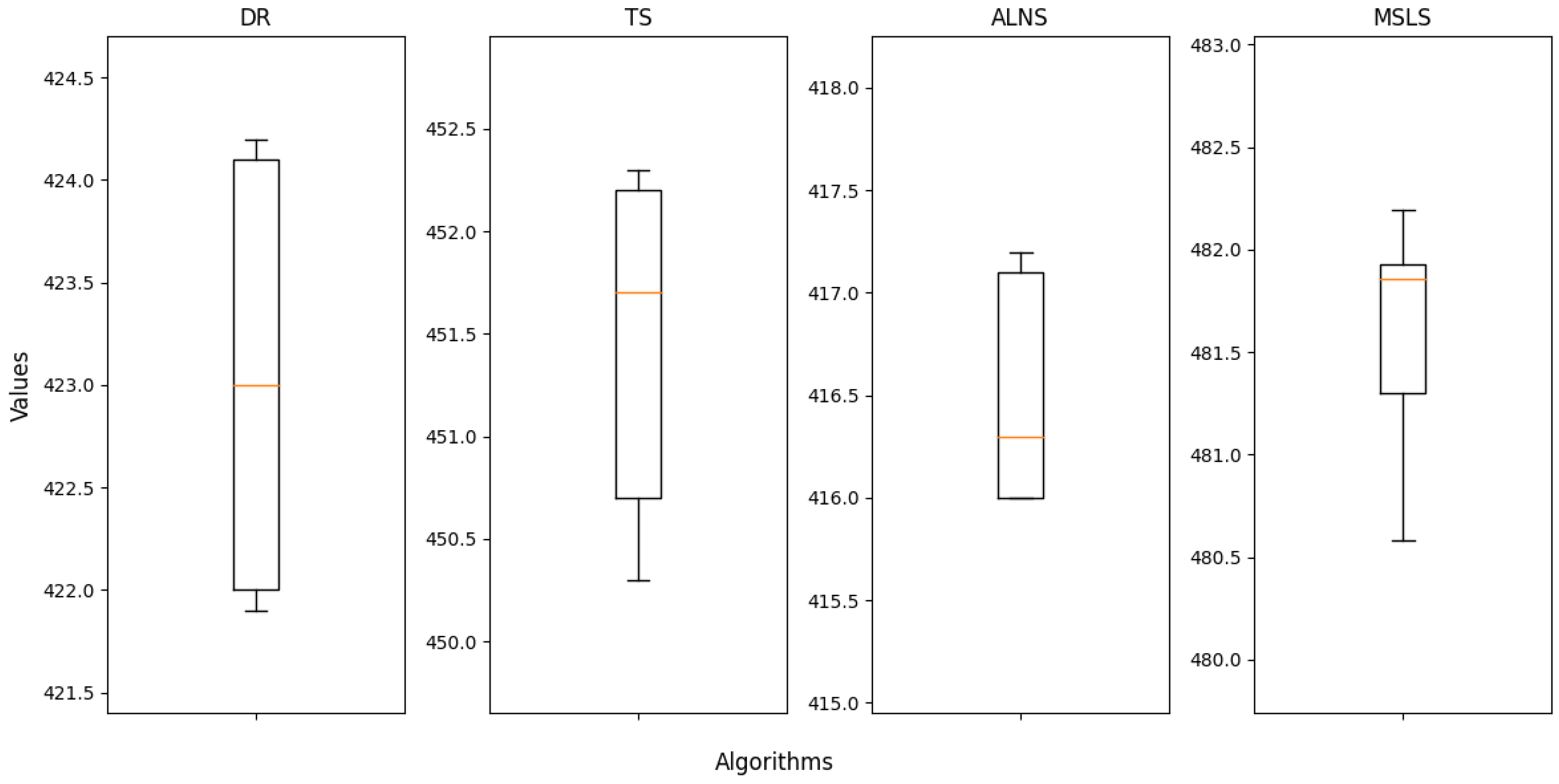
Figure 7.
Objective values obtained by running four algorithms 10 times in scenario M_50_540_14272_454475.
Figure 7.
Objective values obtained by running four algorithms 10 times in scenario M_50_540_14272_454475.
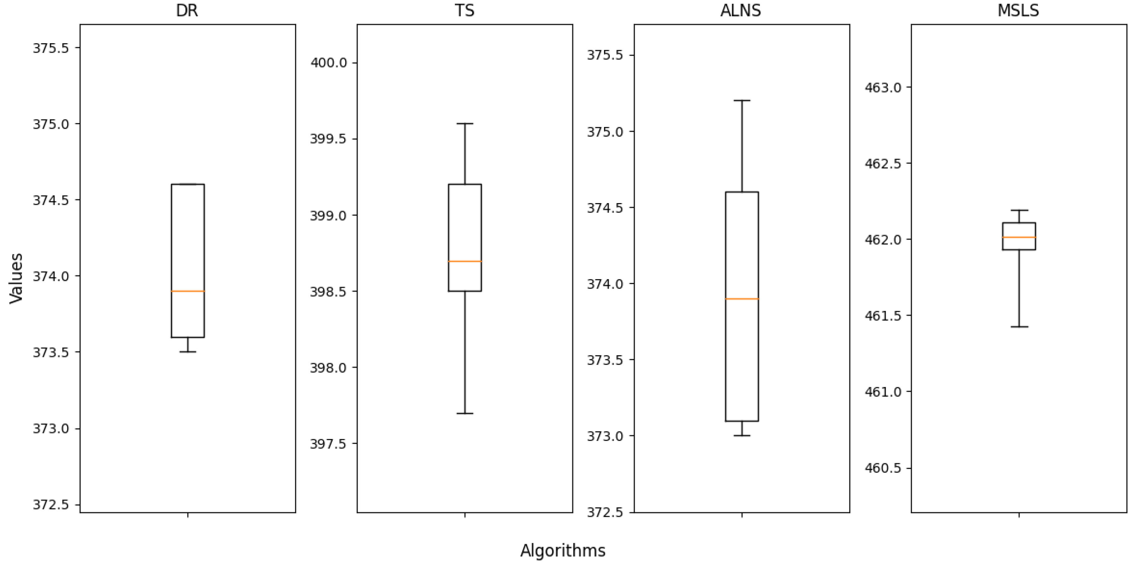
Figure 8.
Objective values obtained by running four algorithms 10 times in scenario L_50_400_19840_684440.
Figure 8.
Objective values obtained by running four algorithms 10 times in scenario L_50_400_19840_684440.
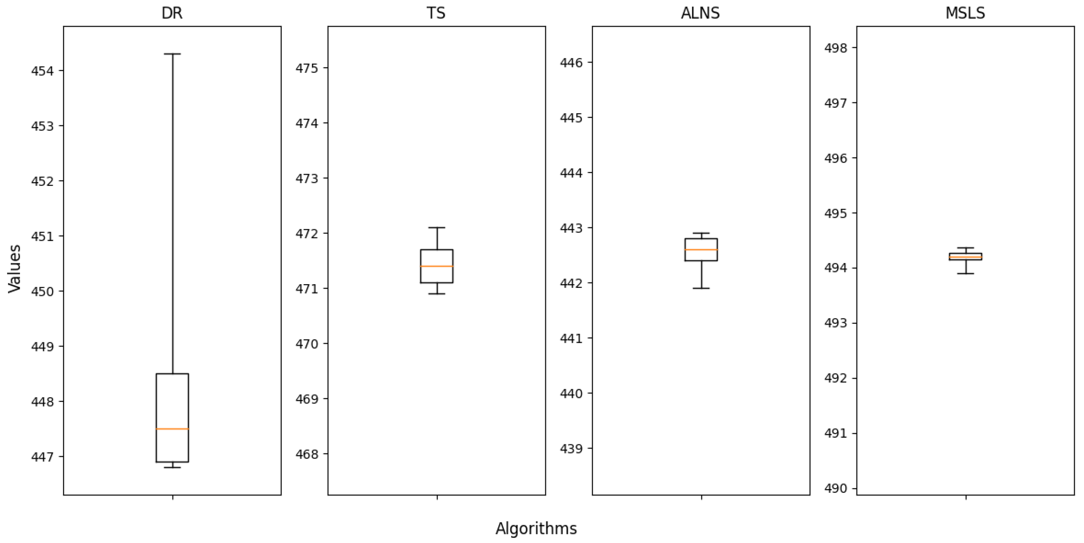
Figure 9.
Objective values obtained by running four algorithms 10 times in scenario L_50_530_27968_894137.
Figure 9.
Objective values obtained by running four algorithms 10 times in scenario L_50_530_27968_894137.
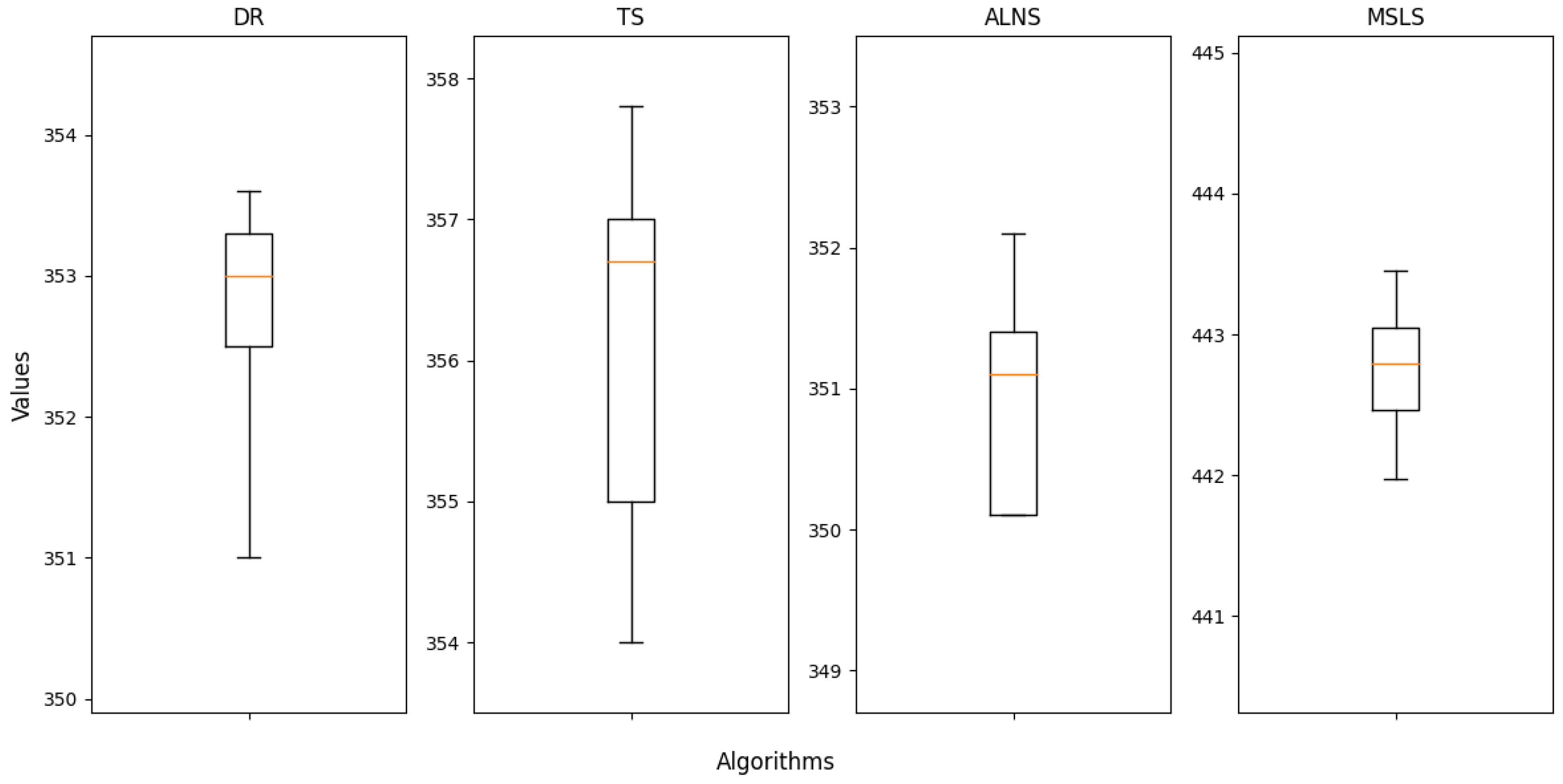
Figure 10.
Iterative graph for four algorithms in small and medium scale scenarios.
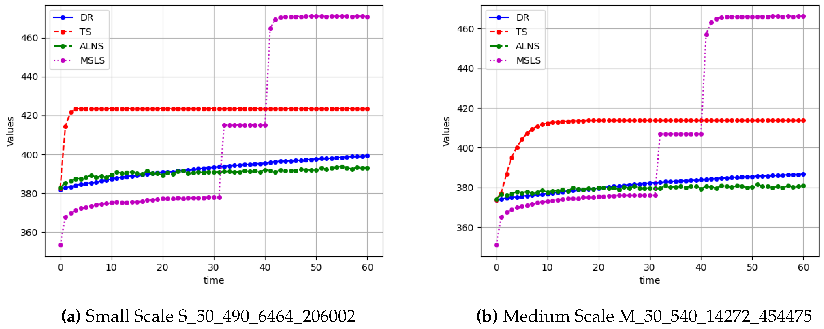
Figure 11.
Iterative graph for four algorithms in large scale scenarios.
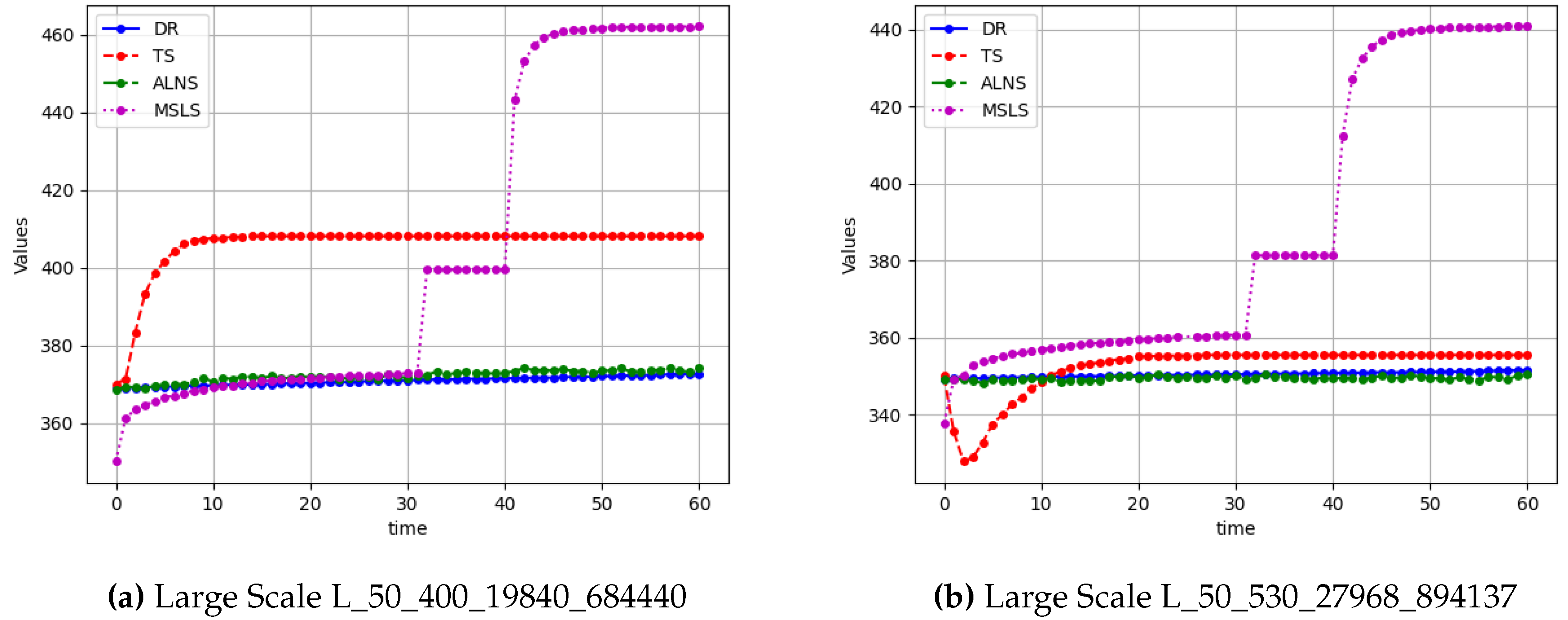

Table 1.
Parameters Used in this Model.
| Parameters | Description |
|---|---|
| T | All task set . |
| Task type which can be or . | |
| Priority for task . | |
| Weighted raio for the idle degree to the objective | |
| V | VTW set . |
| Begining time of VTW . | |
| Ending time of VTW . | |
| The duraiton of VTW | |
| Conflicting VTW list of VTW | |
| Duration of the u-th idle timeslot | |
| All task set supported by VTW , | |
| A | Antenna set |
| All VTWs set belongs antenna , | |
| All task set supported by the antenna , | |
| Function of antenna , which can be | |
| Forbidden time set for , | |
| Chain build time for task | |
| Chain remove time for task | |
| Minimal obervation angle for task | |
| Obervation angle in VTW | |
| O | Orbit set |
| Whatever task is executed in VTW , which can be 0 or 1 |
Table 2.
Computational results between MSLS and other comparison algorithm; The bold data in the table represents the optimal value for each metric across all algorithms.
Table 2.
Computational results between MSLS and other comparison algorithm; The bold data in the table represents the optimal value for each metric across all algorithms.
| DR | TS | |||||||
|---|---|---|---|---|---|---|---|---|
| Scenarios | DDT | TTC | Idle Ratio | Total Score | DDT | TTC | Idle Ratio | Total Score |
| S_47_400_4960_160054 | 1.000 | 0.990 | 0.842 | 467.3 | 1.000 | 1.000 | 0.863 | 472.5 |
| S_49_400_4960_166276 | 1.000 | 0.996 | 0.864 | 472.3 | 1.000 | 1.000 | 0.884 | 476.7 |
| S_50_400_4960_169587 | 1.000 | 0.996 | 0.873 | 474.3 | 1.000 | 1.000 | 0.894 | 478.8 |
| S_50_480_6336_202140 | 0.871 | 0.962 | 0.703 | 410.9 | 0.982 | 1.000 | 0.710 | 438.4 |
| S_50_490_6464_206002 | 0.902 | 0.971 | 0.728 | 423.1 | 0.989 | 1.000 | 0.768 | 451.5 |
| S_50_500_6608_209536 | 0.889 | 0.970 | 0.720 | 418.8 | 0.989 | 1.000 | 0.741 | 445.9 |
| S_50_540_7136_226304 | 0.841 | 0.947 | 0.687 | 400.4 | 0.976 | 1.000 | 0.641 | 423.5 |
| S_52_400_4960_177147 | 1.000 | 1.000 | 0.895 | 478.9 | 1.000 | 1.000 | 0.913 | 482.5 |
| S_50_490_6464_205750 | 0.863 | 0.957 | 0.694 | 407.1 | 0.981 | 1.000 | 0.685 | 433.1 |
| S_50_530_6992_222153 | 0.804 | 0.930 | 0.680 | 389.8 | 0.958 | 1.000 | 0.586 | 408.8 |
| M_47_400_9920_321833 | 0.999 | 0.977 | 0.774 | 452.2 | 1.000 | 1.000 | 0.831 | 466.1 |
| M_49_400_9920_334146 | 0.999 | 0.986 | 0.798 | 458.0 | 1.000 | 1.000 | 0.857 | 471.4 |
| M_50_400_9920_341276 | 1.000 | 0.995 | 0.826 | 464.6 | 1.000 | 1.000 | 0.872 | 474.4 |
| M_50_480_12672_406338 | 0.821 | 0.933 | 0.643 | 386.0 | 0.979 | 1.000 | 0.621 | 420.0 |
| M_50_490_12928_414086 | 0.853 | 0.947 | 0.665 | 398.2 | 0.988 | 1.000 | 0.693 | 436.1 |
| M_50_500_13216_420998 | 0.852 | 0.957 | 0.665 | 399.0 | 0.985 | 1.000 | 0.668 | 430.6 |
| M_50_540_14272_454475 | 0.789 | 0.905 | 0.629 | 374.0 | 0.970 | 1.000 | 0.524 | 398.8 |
| M_52_400_9920_355986 | 1.000 | 1.000 | 0.862 | 472.3 | 1.000 | 1.000 | 0.896 | 479.3 |
| M_50_490_12928_413461 | 0.819 | 0.933 | 0.639 | 385.0 | 0.977 | 1.000 | 0.593 | 414.0 |
| M_50_530_13984_446213 | 0.766 | 0.900 | 0.629 | 369.1 | 0.951 | 1.000 | 0.442 | 378.6 |
| L_47_400_19840_645510 | 0.763 | 0.891 | 0.626 | 366.9 | 1.000 | 1.000 | 0.811 | 462.2 |
| L_49_400_19840_670580 | 0.999 | 0.962 | 0.738 | 443.6 | 1.000 | 1.000 | 0.840 | 468.0 |
| L_50_400_19840_684440 | 0.999 | 0.971 | 0.759 | 448.6 | 1.000 | 1.000 | 0.857 | 471.4 |
| L_50_480_25344_814260 | 0.801 | 0.911 | 0.609 | 373.1 | 0.974 | 1.000 | 0.565 | 407.8 |
| L_50_490_25856_829946 | 0.837 | 0.930 | 0.625 | 385.4 | 0.987 | 1.000 | 0.650 | 427.3 |
| L_50_500_26432_843943 | 0.823 | 0.924 | 0.616 | 380.2 | 0.982 | 1.000 | 0.622 | 420.8 |
| L_50_540_28544_911389 | 0.780 | 0.883 | 0.588 | 361.8 | 0.965 | 1.000 | 0.446 | 382.3 |
| L_52_400_19840_713816 | 1.000 | 0.997 | 0.819 | 463.4 | 1.000 | 1.000 | 0.883 | 476.6 |
| L_50_530_27968_894137 | 0.746 | 0.862 | 0.586 | 352.7 | 0.944 | 1.000 | 0.337 | 356.2 |
| L_50_490_25856_829171 | 0.793 | 0.902 | 0.602 | 369.3 | 0.971 | 1.000 | 0.531 | 400.4 |
| +/=/- | 0/7/23 | 0/2/28 | 0/0/30 | 0/0/30 | 13/12/5 | 0/30/0 | 0/0/30 | 0/0/30 |
| ALNS | MSLS | |||||||
| Scenarios | DDT | TTC | Idle Ratio | Total Score | DDT | TTC | Idle Ratio | Total Score |
| S_47_400_4960_160054 | 0.992 | 0.989 | 0.780 | 453.2 | 1.000 | 1.000 | 0.971 | 494.105 |
| S_49_400_4960_166276 | 0.995 | 0.993 | 0.807 | 459.7 | 1.000 | 1.000 | 0.978 | 495.674 |
| S_50_400_4960_169587 | 0.996 | 0.994 | 0.817 | 461.8 | 1.000 | 1.000 | 0.983 | 496.565 |
| S_50_480_6336_202140 | 0.835 | 0.980 | 0.701 | 405.1 | 0.988 | 1.000 | 0.888 | 475.151 |
| S_50_490_6464_206002 | 0.859 | 0.987 | 0.730 | 416.5 | 0.998 | 1.000 | 0.910 | 481.618 |
| S_50_500_6608_209536 | 0.844 | 0.985 | 0.722 | 411.8 | 0.992 | 1.000 | 0.905 | 479.369 |
| S_50_540_7136_226304 | 0.805 | 0.974 | 0.683 | 394.9 | 0.972 | 1.000 | 0.882 | 470.688 |
| S_52_400_4960_177147 | 0.998 | 0.997 | 0.838 | 466.9 | 1.000 | 1.000 | 0.989 | 497.773 |
| S_50_490_6464_205750 | 0.828 | 0.979 | 0.691 | 401.5 | 0.986 | 1.000 | 0.886 | 474.422 |
| S_50_530_6992_222153 | 0.790 | 0.965 | 0.664 | 387.2 | 0.957 | 1.000 | 0.862 | 463.855 |
| M_47_400_9920_321833 | 0.984 | 0.985 | 0.728 | 441.0 | 1.000 | 1.000 | 0.959 | 491.750 |
| M_49_400_9920_334146 | 0.991 | 0.989 | 0.757 | 448.4 | 1.000 | 1.000 | 0.969 | 493.895 |
| M_50_400_9920_341276 | 0.993 | 0.992 | 0.771 | 452.1 | 1.000 | 1.000 | 0.975 | 495.063 |
| M_50_480_12672_406338 | 0.802 | 0.977 | 0.636 | 385.3 | 0.976 | 1.000 | 0.863 | 467.799 |
| M_50_490_12928_414086 | 0.824 | 0.984 | 0.672 | 397.5 | 0.989 | 1.000 | 0.887 | 475.221 |
| M_50_500_13216_420998 | 0.813 | 0.982 | 0.661 | 393.1 | 0.982 | 1.000 | 0.885 | 473.439 |
| M_50_540_14272_454475 | 0.773 | 0.968 | 0.613 | 374.0 | 0.955 | 1.000 | 0.855 | 461.950 |
| M_52_400_9920_355986 | 0.996 | 0.996 | 0.795 | 457.7 | 1.000 | 1.000 | 0.985 | 496.952 |
| M_50_490_12928_413461 | 0.793 | 0.976 | 0.627 | 381.5 | 0.969 | 1.000 | 0.858 | 465.495 |
| M_50_530_13984_446213 | 0.750 | 0.960 | 0.593 | 364.6 | 0.934 | 1.000 | 0.824 | 451.598 |
| L_47_400_19840_645510 | 0.981 | 0.984 | 0.692 | 432.9 | 1.000 | 1.000 | 0.952 | 490.422 |
| L_49_400_19840_670580 | 0.986 | 0.989 | 0.721 | 440.2 | 1.000 | 1.000 | 0.965 | 492.978 |
| L_50_400_19840_684440 | 0.987 | 0.991 | 0.730 | 442.5 | 1.000 | 1.000 | 0.971 | 494.183 |
| L_50_480_25344_814260 | 0.783 | 0.976 | 0.595 | 373.2 | 0.962 | 1.000 | 0.845 | 461.355 |
| L_50_490_25856_829946 | 0.809 | 0.983 | 0.631 | 386.2 | 0.982 | 1.000 | 0.873 | 470.990 |
| L_50_500_26432_843943 | 0.798 | 0.981 | 0.617 | 381.1 | 0.971 | 1.000 | 0.870 | 468.280 |
| L_50_540_28544_911389 | 0.758 | 0.965 | 0.569 | 361.9 | 0.938 | 1.000 | 0.832 | 453.982 |
| L_52_400_19840_713816 | 0.991 | 0.994 | 0.762 | 450.0 | 1.000 | 1.000 | 0.982 | 496.370 |
| L_50_530_27968_894137 | 0.732 | 0.955 | 0.546 | 351.0 | 0.920 | 1.000 | 0.794 | 442.756 |
| L_50_490_25856_829171 | 0.774 | 0.973 | 0.581 | 368.3 | 0.957 | 1.000 | 0.841 | 459.631 |
| +/=/- | 0/0/30 | 0/0/30 | 0/0/30 | 0/0/30 | - | - | - | - |
Disclaimer/Publisher’s Note: The statements, opinions and data contained in all publications are solely those of the individual author(s) and contributor(s) and not of MDPI and/or the editor(s). MDPI and/or the editor(s) disclaim responsibility for any injury to people or property resulting from any ideas, methods, instructions or products referred to in the content. |
© 2024 by the authors. Licensee MDPI, Basel, Switzerland. This article is an open access article distributed under the terms and conditions of the Creative Commons Attribution (CC BY) license (http://creativecommons.org/licenses/by/4.0/).
Copyright: This open access article is published under a Creative Commons CC BY 4.0 license, which permit the free download, distribution, and reuse, provided that the author and preprint are cited in any reuse.


