
Submitted:
18 November 2024
Posted:
20 November 2024
You are already at the latest version
Abstract
The study of solutions to differential equations is crucial in addressing a wide range of practical problems, and the Bessel function plays a critical role in this field. As a result, the theory of Bessel functions and their applications is a rich and complex subject. The purpose of this paper is to introduce a new type of generalized Bessel function and explore its applications. Specifically, the paper derives formulas for fractional integrals and derivatives using the Riemann-Liouville approach, and presents a novel form of the fractional kinetic equation that involves a first-order generalized Bessel function. The paper also discusses the broad versatility of the generalized Bessel function and its potential to generate both known and new results. Several figures are included to illustrate the properties of the solutions derived.
Keywords:
Special functions
; Bessel functions
; fractional differential equations
; Fractional kinetic equations
MSC: 33C10; 44A10; 34A08
1. Introduction
In contemporary engineering and physics, a profound understanding of applied mathematics, specifically pertaining to the fundamental characteristics of special functions, is indispensable. Special functions play a crucial role in various applications within the realm of physical sciences. The discipline of analysis, devoted to the examination of these specialized functions, traces its roots back to the early days of calculus, making it one of the most venerable fields of study. In recent decades, the discovery of novel special functions and their application to unexplored mathematical domains has reignited enthusiasm and rekindled scholarly curiosity in this area.
The investigation of Bessel functions holds significant relevance in the examination of crucial differential equations, (see for example [1]). These functions, rooted in Bessel function theory, find widespread application in diverse fields such as information theory, radiophysics, hydrodynamics, and nuclear physics. Notably, there has been a resurgence of interest in the exploration of Bessel functions within the context of fractional calculus theory, we may mention for example [2,3,4,5,6,7] and references therein.
Fractional calculus, which extends the concepts of differentiation and integration to arbitrary orders, is an intriguing branch of applied mathematics that has recently received a significant amount of attention from mathematicians and physicists. It is a powerful tool for studying a wide range of scientific problems, with many breakthroughs in control theory, hydrology, chaotic dynamics, kinetic theories, biophysics, bioengineering, quantum mechanics, diffusion processes, statistical mechanics, polymer sciences, thermodynamics, signal and image processing, astrophysics, and cosmology where many of the associated models amount to replace the time and space derivatives in an evolution equation with fractional derivatives of real orders (see [8,9,10,11,12,13,14,15]).
This subfield dates back to the late 17th century and evolved from the traditional definitions of calculus integral and derivative operators in much the same way that fractional exponents evolved from integer exponents. Several authors have stated that fractional-order operators are not only more suitable for modelling but also have advantages over integer-order operators.
It is important to recognize that there are multiple definitions for fractional-order derivatives, including divided-difference and infinite-sum types, such as the Grünwald-Letnikov fractional derivative, Weyl, Caputo, Feller, Riesz, Erdelyi-Kober fractional derivatives, and others. However, when it comes to fractional integration, the Riemann-Liouville (RL) and Caputo operators remain the most widely utilized and well-known methods. In modeling problems involving the concepts of nonlocality and memory effect, which are not well explained by integer-order calculus, fractional calculus stands out. Indeed, fractional calculus deals with the concept of the derivative operator, which is a local operator in integer order calculus but non-local in fractional calculus [16,17].
Indeed, fractional derivatives and integrals offer a more precise description of complex physical systems. These operators have been successfully incorporated into classical and quantum dynamical theories, demonstrating their utility in exploring novel fractal concepts [18]. They have introduced fresh perspectives and bridged gaps in traditional calculus that have yet to be fully assimilated or comprehended. Fractional calculus has proven effective in solving various physics problems, spanning classical to quantum domains. It is now recognized as a powerful tool for characterizing non-equilibrium complex systems exhibiting scale-invariant properties, dissipation, and long-range correlations that defy representation using traditional analytic functions and ordinary differential operators.
Presently, there are two prevailing approaches to describing fractional calculus. The first approach, known as the Riemann-Liouville approach, involves iteratively applying the integral operator n times and replacing it with a single integral using the well-known Cauchy formula. In this formulation, the factorial is replaced with the Gamma function, enabling the definition of fractional integrals for non-integer orders. The Riemann and Caputo fractional derivatives have also been rigorously defined using integrals [19]. The second trend in fractional derivatives was pioneered by Grunwald-Letnikov. Their method involves iteratively applying the derivative n times and then fractionalizing the binomial coefficients using the Gamma function.
As they are used to model relevant systems, fractional differential equations have grown in popularity across a wide range of applied sciences. These equations play a vital role not just in the field of mathematics, but also in physics, control systems, dynamical systems, and engineering. They make it easier to create mathematical models that represent a wide variety of physical phenomena. Kinetic equations, in particular, are fundamental in mathematical physics and natural science because they describe the continuous motion of substances. As a result, as seen in previous research [6,20,21,22,23,24,25,26,27,28,29,30,31,32,33,34], there has been a pursuit of extending and generalising fractional kinetic equations by incorporating diverse fractional calculus operators.
The structure of this paper is outlined as follows. Section 2 gathers the necessary concepts and definitions, and additionally introduces new and more generalized Bessel functions in the same section. In Section 3, we derive new Riemann-Liouville fractional integral and derivative formulas for the defined Bessel function. Section 4 is divided into three subsections. In SubSection 4.1, we explore the solutions of a novel type of fractional kinetic equation related to the generalized Bessel function. SubSection 4.2 presents various special cases of our main results. The graphical interpretation of the main findings is the focus of SubSection 4.3. Finally, concluding remarks are provided in Section 5.
2. Preliminaries and Basic Concepts
It is important to note that Riemann-Liouville and Caputo fractional derivatives are nonlocal operators with convolutional integrals with weak singularities. In the physical system, these non-local fractional derivatives introduce inherent memory and genetic effects.
The RL fractional integral and derivative of order are defined as follows (see, e.g., [8]):
- The left-side RL fractional integral
- The right-side RL fractional integral
- The left-side RL fractional derivative
- The right-side RL fractional derivative
Lemma 2.1.
Let and then
and
We now review the essential definitions that will be used in the sequel.
Definition 2.1.
Mittag-Leffler functions arise as inherent solutions to equations involving fractional order differentials and integrals.
In 1903, Mittag-Leffler [37] introduced and named the function after himself, defining it using a power series representation.
Wiman generalised this function in 1905 [38] as
In the present paper, we take into account a brand-new generalised Bessel function with the following form:
where and denotes the generalized pochhammer symbol (see, e.g [39]).
Remark 2.1.
The series (2.10) generalizes many special cases as follows
- (i)
- Putting and in (2.10), we obtain the generalized Bessel function of the first kind, defined by [40].
- (ii)
- Setting and in (2.10), the generalized Bessel function reduced to the familiar Bessel function of the first kind of order , given by [40].
- (iii)
- If we put and in (2.10), then the generalized Bessel function reduced to generalized type of modified Bessel function of the first kind, defined by [41].
- (iv)
- Setting and in (2.10), we have the familiar modified Bessel function of the first kind of order , given by [40].
- (v)
- Putting and in (2.10), we obtain the spherical Bessel function of order , defined by [40].
- (vi)
- Setting and in (2.10), we the generalized Bessel function reduced towhere is the generalized matland Bessel function defined by [42]
- (vii)
- Putting and in (2.10), we the generalized Bessel function reduced towhere is the familiar matland Bessel function given by [43].
Inspired by the preceding discussions and the existing literature on Bessel functions, this study intends to conduct additional research involving the generalised Bessel function (2.10). To begin, we provide fractional integral and differential formulations, as shown below.
3. Fractional Calculus Approach of
In this section, we derive the Riemann-Liouville fractional integration and fractional differentiation of the recently defined generalized Bessel function, denoted as . The obtained results are presented as follows.
3.1. Fractional Integral Forms
Theorem 3.1.
Suppose λ and η are complex numbers such that the real part of λ is greater than 0 and the real part of η is greater than Additionally, assume that the conditions stated in equation (2.10) are satisfied. Under these circumstances, the following formula for fractional integration is valid.
Proof.
Denoting the left-hand side of (3.1) by Using (2.10), we obtain
Using (2.5) of Lemma 2.1, we get
In view of the definition of the Fox-Wright function (2.7), we have
as desired. □
Theorem 3.2.
Suppose λ and η are complex numbers such that the real part of λ is greater than 0 and the real part of η is greater than Additionally, assume that the conditions stated in equation (2.10) are satisfied. Under these circumstances, the following formula for fractional integration is valid.
Proof.
Denoting the left-hand side of (3.1) by . Using (2.10), we have
Using (2.6) of Lemma 2.1, we get
In view of the definition of the Fox-wright function (2.7), we arrive at the desired result. □
3.2. Fractional Derivative Forms
Theorem 3.3.
Let be such that and the conditions given in (2.10) are satisfied, then the following fractional integral formula holds true
Proof.
Denoting the left-hand side of (3.3) by Using (2.10) and (2.3), we obtain
Using (2.5) of Lemma 2.1, we have
after some simplification
In view if the definition of the Fox-wright function (2.7), we have
as required. □
Theorem 3.4.
Let be such that and the conditions given in (2.10) are satisfied, then the following fractional integral formula holds true
Proof.
Denoting the left-hand side of (3.4) by . Using (2.10) and (2.4), we have
Using (2.6) of Lemma 2.1, we obtain
Using the identity we have
In view of the definition of the Fox-wright function (2.7), we arrive at the desired result. □
4. Fractional Kinetic Equation
In light of the kinetic equation’s effectiveness and importance in certain astrophysical problems, the authors devise a new generalised form of the fractional kinetic equation involving a newly defined Bessel function of the first kind.
Haubold and Mathai [21] have formulated a functional differential equation that relates the rate of reaction change, the rate of destruction, and the rate of production in the following manner:
where is the rate of reaction, is the rate of destruction, is the rate of production, and
When spatial fluctuations or inhomogeneities in the quantity are ignored, Haubold and Mathai studied a special case of the equation, which is given by the equation.
together with the initial condition that , is the number of density of species i at time If the index i is dropped and the typical kinetic equation (4.2) is integrated, we receive
where is the special case of the Riemann-Liouville integral operator 0 defined in (2.1).
Haubold and Mathai [21] have given the fractional generalization of the standard kinetic equation (4.3) as
Then the solution for is a Mittag-Leffler function
In addition, Saxena and Kalla [22] thought about the subsequent fractional kinetic equation
where
We now utilize the Laplace transform technique to obtain the solution for an integral equation more encompassing than the one referenced as (4.6). This is achieved by employing the findings presented in the work by [32].
where
In the following subsection, we solve novel fractional kinetic equations that incorporate the recently introduced generalised Bessel function, as defined in Equation (4.6). Furthermore, we create a variety of distinct special scenarios.
4.1. Solution of Fractional Kinetic Equation
Within this subsection, we explore the resolution of the fractional kinetic equation linked to the generalized Bessel function outlined in section 2.
Remark 4.1.
The solutions we are about to deduce for the appropriate fractional kinetic equations will be ascertained using the generalized Mittag-Leffler function introduced by [38], as defined in Equation (2.9).
Theorem 4.1.
If and then the solution of the equation
is given by the following formula:
where is the generalized Mittag-Leffler function.
Proof.
By employing the Laplace transform to both sides of (4.9) and utilizing (4.7), we arrive at the result
Hence,
Therefore,
Taking Laplace inverse of (4.11) and using , we obtain
In view of (2.9), we get the required result. □
Theorem 4.2.
If and then the solution of the equation
is given by the following formula:
Proof.
Applying the laplace transform to the both sides of (4.12), and using (4.7), we obtain
Hence,
Therefore,
Taking Laplace inverse of (4.14) and using , we obtain
this completes the proof of theorem 4.1. □
Theorem 4.3.
If and then the formula
is a solution of the fractional kinetic equation
Proof.
The proof of theorem 4.3 is parallel to theorems 4.1 and 4.2, so details of the proof are omitted. □
4.2. Special Cases
- (i)
-
Choosing and the generalized Bessel function (2.10), reduced to the generalized type of Bessel function of the first kind, as we mentioned in (2.11).Then theorems 4.1, 4.2, and 4.3 reduce to the following corollaries.Corollary 4.1. If and then the solution of the equationis given by the following formula:Corollary 4.2. If and then the solution of the equationis given by the following formula:Corollary 4.3. If and then the formulais a solution of the fractional kinetic equation
- (ii)
-
Setting and the generalized Bessel function (2.10), reduced to Bessel function of the first kind, as mentioned in (2.12).Then theorems 4.1, 4.2, and 4.3 reduce to the following corollaries.Corollary 4.4. If andthen the solution of the equationis given by the following formula:Corollary 4.5. If andthen the solution of the equationis given by the following formula:Corollary 4.6. If and then the formulais a solution of the fractional kinetic equation
- (iii)
-
Choosing and the generalized Bessel function (2.10), reduced to generalized type of modified Bessel function of the first kind, as mentioned in (2.13).Then theorems 4.1, 4.2, and 4.3 reduce to the following corollaries.Corollary 4.7. If andthen the solution of the equationis given by the following formula:Corollary 4.8. If andthen the solution of the equationis given by the following formula:Corollary 4.9. If and then the formulais a solution of the fractional kinetic equation
- (iv)
-
Choosing and the generalized Bessel function (2.10), reduced to modified Bessel function of the first kind, as mentioned in (2.14).Then theorems 4.1, 4.2, and 4.3 reduce to the following corollaries.Corollary 4.10. If andthen the solution of the equationis given by the following formula:Corollary 4.11. If andthen the solution of the equationis given by the following formula:Corollary 4.12. If and then the formulais a solution of the fractional kinetic equation
- (v)
-
Choosing and the generalized Bessel function (2.10), reduced to spherical Bessel function, as mentioned in (2.15).Then theorems 4.1, 4.2, and 4.3 reduce to the following corollaries.Corollary 4.13. If andthen the solution of the equationis given by the following formula:Corollary 4.14. If andthen the solution of the equationis given by the following formula:Corollary 4.15. If and then the formulais a solution of the fractional kinetic equation
- (vi)
-
Setting and the generalized Bessel function (2.10), reduced towhere is the generalized matland Bessel function given in (2.16).Then Theorems 4.1, 4.2, and 4.3 reduce to the following corollaries.Corollary 4.16. If and then the solution of the equationis given by the following formula:Corollary 4.17. If and then the solution of the equationis given by the following formula:Corollary 4.18. If and then the formulais a solution of the fractional kinetic equation
- (vii)
-
Setting and the generalized Bessel function (2.10), reduced towhere is matland Bessel function given in (2.17).Then theorems 4.1, 4.2, and 4.3 reduce to the following corollaries.Corollary 4.19. If and then the solution of the equationis given by the following formula:Corollary 4.20. If and then the solution of the equationis given by the following formula:Corollary 4.21. If and then the formulais a solution of the fractional kinetic equation
4.3. Graphical Interpretation
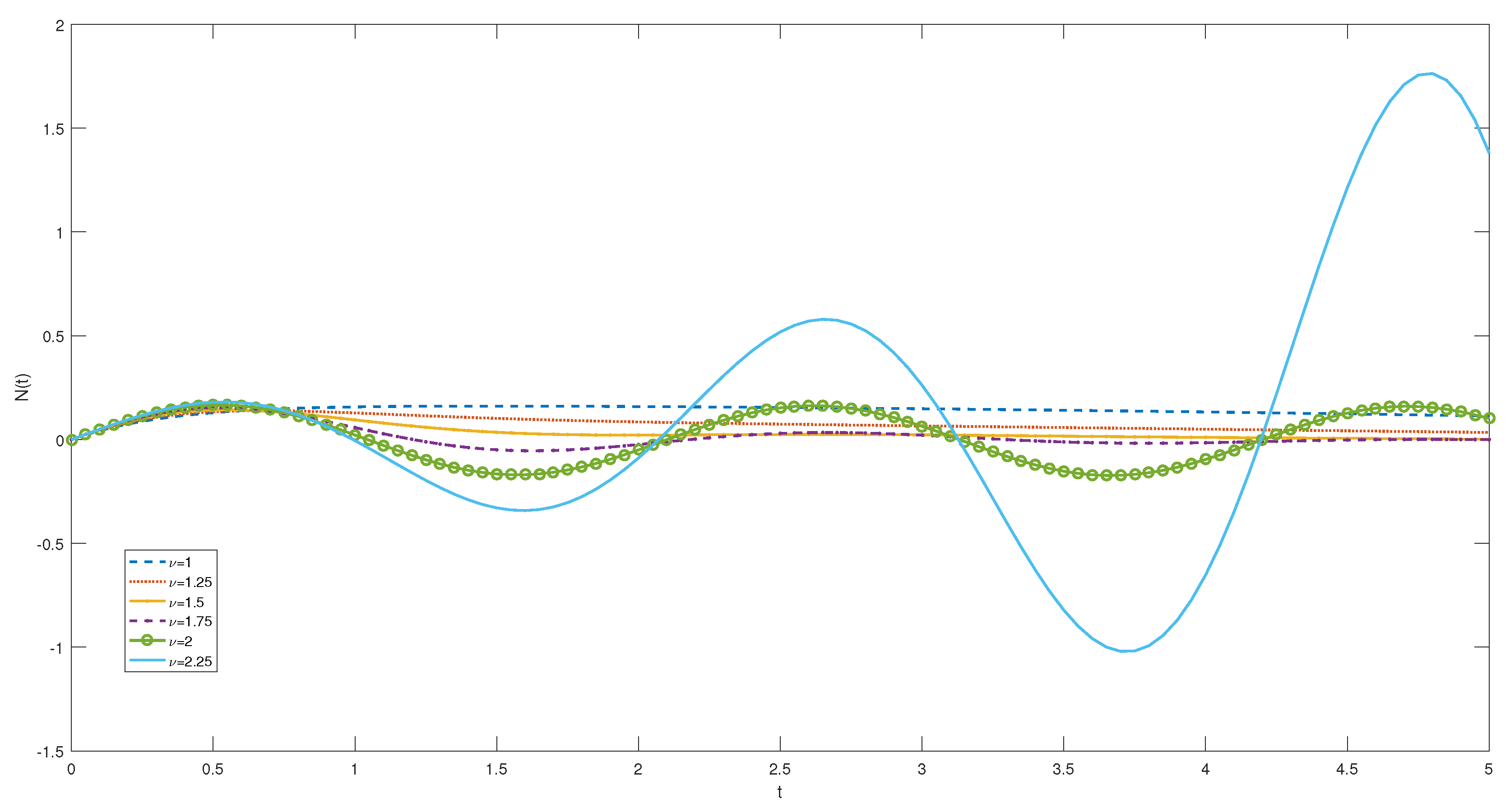
In this subsection, we present graphical representations that illustrate the main results obtained in Theorems 4.1, 4.2, and 4.3. These graphs depict the solution curves of equation (4.9) for various parameter values. Specifically, we consider the parameters , , , and . The solution curves are shown in Figure 1 for the time interval , where and . Furthermore, Figure 2 presents the curves for the same parameter values, but with and , and for the time interval . Additionally, Figure 3 displays the curves for the time interval , with and .
From these figures, it is evident that at the initial time for different parameter values. Moreover, it is observed that selecting in Theorems (2.16) and (2.18) yields identical solutions. Our observations also reveal that exhibits both positive and negative values for different parameter settings.
5. Conclusion
The inclusion of convolution integrals with power-law or exponential-law memory kernels through fractional derivatives enhances the significance of fractional differential equations in elucidating the memory effects exhibited by complex systems.
The objective of this paper was to introduce a novel generalized Bessel function and establish formulas for fractional integrals and fractional derivatives. We conducted a comprehensive investigation of several intriguing fractional kinetic equations, considering a range of special functions [22,29,30,31,32]). Furthermore, we proposed a new and generalized solution for the fractional kinetic equation associated with the introduced generalized Bessel function, which we analyzed utilizing the Laplace integral transform technique. The main findings can serve as a basis for constructing a diverse set of kinetic equations and their potential solutions. Based on our graphical results, it can be concluded that exhibits either positive or negative values across different parameter values and time intervals. The results obtained in this study have significant implications, as they have the potential to generate numerous established findings and potentially uncover new ones.
Our future work will be dedicated to further exploring and studying the recently introduced generalized Bessel function in the realm of solving fractional differential equations. We recognize the potential of this function in offering solutions to a wide array of fractional differential equations, which necessitates thorough investigation. Our focus will be on examining its properties, analyzing its behavior under different parameter configurations, and assessing its applicability across various scientific and engineering domains. Furthermore, we will investigate numerical methods and algorithms that can efficiently compute solutions involving the generalized Bessel function (see our previous work [6]). The aim of this research is to enhance the understanding and utilization of this function in solving intricate fractional differential equations, thereby advancing the field of fractional calculus.
Conflicts of Interest
The authors declare no conflict of interest.
References
- J. Niedziela, Bessel functions and their applications, Knoxville: University of Tennessee, 2008.
- M. Izadi, and C. Cattani, "Generalized Bessel polynomial for multi-order fractional differential equations," Symmetry, vol. 12(8), p. 1260, 2020.
- Droghei, R. (2021). On a solution of a fractional hyper-Bessel differential equation by means of a multi-index special function. Fractional Calculus and Applied Analysis, 24(5), 1559-1570.
- Dubovski, P. B. and Slepoi, J. (2021). Analysis of solutions of some multi-term fractional Bessel equations. Fractional Calculus and Applied Analysis, 24(5), 1380-1408.
- Agarwal, R., Kumar, N., Parmar, R. K. and Purohit, S. D. (2021). Fractional calculus operator of the product of generalized modified Bessel function of the second type. Communications of the Korean Mathematical Society, 36(3), 557-573.
- Abul-Ez, M., Zayed, M. and Youssef, A. (2021). Further Developments of Bessel Functions via Conformable Calculus with Applications. Journal of Function Spaces, 2021.
- H. Dehestani, Y. Ordokhani, and M. Razzaghi, "Fractional-order Bessel functions with various applications," Applications of Mathematics, vol. 64(6), pp. 637-662, 2019.
- Samko, S. G., Kilbas, A. A. and Marichev, O. I. (1993). Fractional integrals and derivatives (Vol. 1). Yverdon-les-Bains, Switzerland: Gordon and Breach Science Publishers, Yverdon.
- Podlubny, I. (1998). Fractional differential equations: an introduction to fractional derivatives, fractional differential equations, to methods of their solution and some of their applications. Elsevier.
- Hilfer, R. (Ed.). (2000). Applications of fractional calculus in physics (Vol. 35, No. 12, pp. 87-130). Singapore: World scientific.
- Magin, R. L. (2004). Fractional calculus in bioengineering, part 1. Critical Reviews™ in Biomedical Engineering, 32(1).
- Agrawal, O. P. (2004). A general formulation and solution scheme for fractional optimal control problems. Nonlinear Dynamics, 38(1-4), 323-337.
- Kilbas, A. A., Srivastava, H. M. and Trujillo, J. J. (2006). Theory and applications of fractional differential equations (Vol. 204). elsevier.
- M. Abul-Ez, M. Zayed, A. Youssef and M. De la Sen, "On conformable fractional Legendre polynomials and their convergence properties with applications, Alexandria Engineering Journal, vol. 59(6), pp. 5231-5245, 2020.
- M. Abul-Ez, M. Zayed and A. Youssef "Further study on the conformable fractional Gauss hypergeometric function, Aims Mathematics, vol. 6(9), pp. 10130-10163, 2021.
- Teodoro, G. S., Machado, J. T. and De Oliveira, E. C. (2019). A review of definitions of fractional derivatives and other operators. Journal of Computational Physics, 388, 195-208.
- Mainardi, F. (2010). Fractional calculus and waves in linear viscoelasticity: an introduction to mathematical models. World Scientific.
- El-Nabulsi, R. A. (2009). Fractional Dirac operators and deformed field theory on Clifford algebra. Chaos, Solitons & Fractals, 42(5), 2614-2622.
- Ghanbari, B. and Gómez-Aguilar, J. F. (2019). Analysis of two avian influenza epidemic models involving fractal-fractional derivatives with power and Mittag-Leffler memories. Chaos: An Interdisciplinary Journal of Nonlinear Science, 29(12), 123113.
- Singh, Y., Gill, V., Singh, J., Kumar, D. and Khan, I. (2021). Computable generalization of fractional kinetic equation with special functions. Journal of King Saud University-Science, 33(1), 101221.
- Haubold, H. J. and Mathai, A. M. (2000). The fractional kinetic equation and thermonuclear functions. Astrophysics and Space Science, 273(1), 53-63.
- Saxena, R. K. and Kalla, S. L. (2008). On the solutions of certain fractional kinetic equations. Applied Mathematics and Computation, 199(2), 504-511.
- Lu, M. and Liu, J. (2021). On a class of stochastic fractional kinetic equation with fractional noise. Advances in Difference Equations, 2021(1), 1-33.
- Kumar Bansal, M., Kumar, D., Harjule, P. and Singh, J. (2020). Fractional kinetic equations associated with incomplete I-functions. Fractal and Fractional, 4(2), 19.
- Chaurasia, V. B. L. and Pandey, S. C. (2008). On the new computable solution of the generalized fractional kinetic equations involving the generalized function for the fractional calculus and related functions. Astrophysics and space science, 317(3), 213-219.
- Chaurasia, V. B. L. and Singh, Y. (2015). A novel computable extension of fractional kinetic equations arising in astrophysics. International Journal of Advances in Applied Mathematics and Mechanics, 3(1), 1-9.
- Nisar, K. S. and Qi, F. (2018). On solutions of fractional kinetic equations involving the generalized-Bessel function. Note di Matematica, 37(2), 11-20.
- Saichev, A. I. and Zaslavsky, G. M. (1997). Fractional kinetic equations: solutions and applications. Chaos: An Interdisciplinary Journal of Nonlinear Science, 7(4), 753-764.
- Agarwal, P., Chand, M. and Singh, G. (2016). Certain fractional kinetic equations involving the product of generalized k-Bessel function. Alexandria Engineering Journal, 55(4), 3053-3059.
- Agarwal, P., Chand, M., Baleanu, D., O’Regan, D. and Jain, S. (2018). On the solutions of certain fractional kinetic equations involving k-Mittag-Leffler function. Advances in Difference Equations, 2018(1), 249.
- Kumar, D., Purohit, S. D., Secer, A. and Atangana, A. (2015). On generalized fractional kinetic equations involving generalized Bessel function of the first kind. Mathematical Problems in Engineering, 2015.
- Singh, G., Agarwal, P., Chand, M. and Jain, S. (2018). Certain fractional kinetic equations involving generalized k-Bessel function. Transactions of A. Razmadze Mathematical Institute, 172(3), 559-570.
- Tassaddiq, A., & Srivastava, R. (2023). New Results Involving the Generalized Krätzel Function with Application to the Fractional Kinetic Equations. Mathematics, 11(4), 1060.
- Niyaz, M., Soliman, A. H., & Bakhet, A. (2023, April). Investigation of Fractional Calculus for Extended Wright Hypergeometric Matrix Functions. In Abstract and Applied Analysis (Vol. 2023). Hindawi.
- Fox, C. (1961). The G and H functions as symmetrical Fourier kernels. Transactions of the American Mathematical Society, 98(3), 395-429.
- Wright, E. M. (1935). The asymptotic expansion of the generalized hypergeometric function. Journal of the London Mathematical Society, 1(4), 286-293.
- Mittag-Leffler, G. M. (1903). Sur la nouvelle fonction Eα(x). CR Acad. Sci. Paris, 137(2), 554-558.
- Wiman, A. (1905). Über den Fundamentalsatz in der Teorie der Funktionen Ea(x). Acta Mathematica, 29(1), 191-201.
- Rainville, Earl D. Special Functions. (1960). Chelsea, New York (1969).
- Baricz, Á. (2010). Generalized Bessel functions of the first kind. Springer.
- Galué, L. (2003). A generalized Bessel function. Integral Transforms and Special Functions, 14(5), 395-401.
- Singh, M., Khan, M. A., Khan, A. H. and Khan, A. H. (2014). On some properties of a generalization of Bessel-Maitland function. Int. J. Math. Trends and Tech, 14(1), 46-54.
- Marichev, O. I. (1983). Handbook of integral transforms of higher transcendental functions; theory and algorithmic tables (No. 04; QA432, M3.).
Figure 1.
Solution of Theorem 4.1 for ; ; and and with .
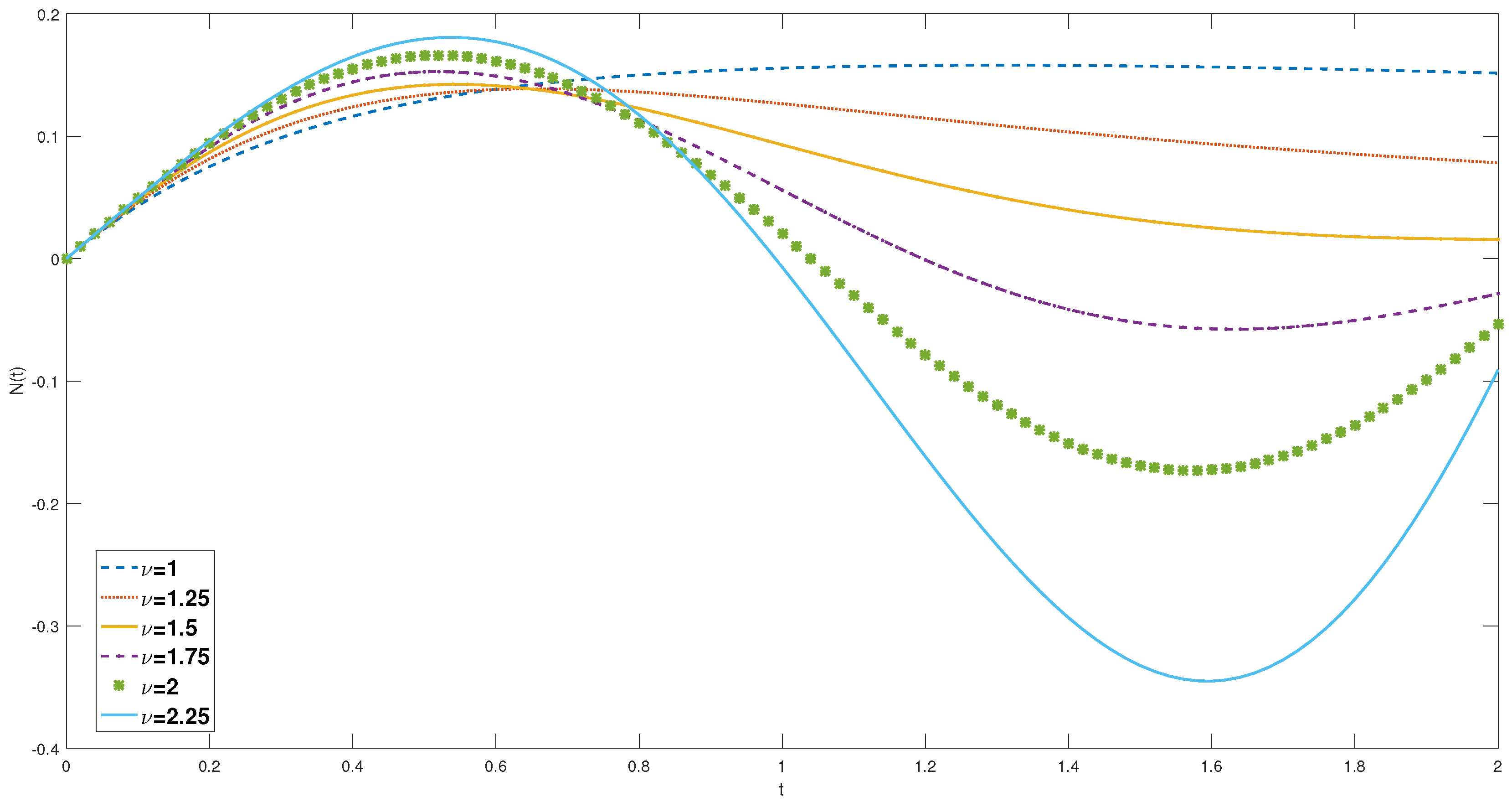
Figure 2.
Solution of Theorem 4.1 for ; ; ; and and with .
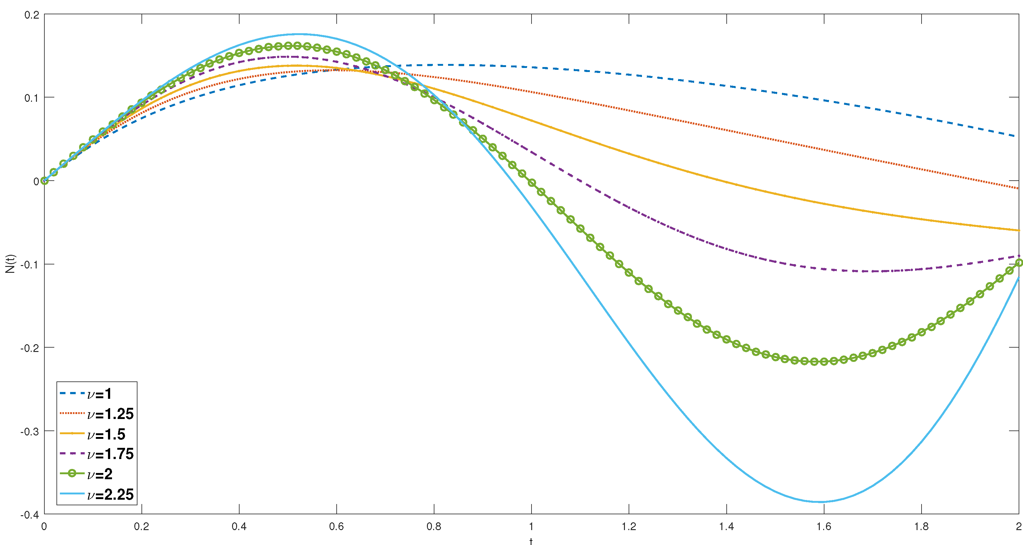
Figure 3.
Solution of Theorem 4.1 for ; ; ; and and with .
Disclaimer/Publisher’s Note: The statements, opinions and data contained in all publications are solely those of the individual author(s) and contributor(s) and not of MDPI and/or the editor(s). MDPI and/or the editor(s) disclaim responsibility for any injury to people or property resulting from any ideas, methods, instructions or products referred to in the content. |
© 1996 by the authors. Licensee MDPI, Basel, Switzerland. This article is an open access article distributed under the terms and conditions of the Creative Commons Attribution (CC BY) license (https://creativecommons.org/licenses/by/4.0/).
Copyright: This open access article is published under a Creative Commons CC BY 4.0 license, which permit the free download, distribution, and reuse, provided that the author and preprint are cited in any reuse.


