Geometric Nature of the Turánian of Modified Bessel Function of the First Kind

1. Introduction

The properties of Bessel functions hold significant importance across multiple domains, including mathematical physics and engineering, quantum mechanics, signal processing, fluid dynamics, electromagnetism, acoustics, and heat conduction. In [1], Baricz et al. introduced conditions for normalized Bessel function to exhibit convexity and starlikeness within the unit disk, resolving an open problem and presenting a novel inequality for the Euler $\Gamma$ function. Sufficient conditions for the univalence of normalized generalized Bessel functions in the unit disk are established by Prajapat in [2]. In [3], Mondal and Swaminathan explored the geometric properties of generalized Bessel functions, yielding various conditions for close-to-convexity, starlikeness, and convexity. Conditions for the close-to-convexity of special functions, including Bessel functions, are deduced by Baricz and Szasin [4], utilizing results on transcendental entire functions and Pólya’s Theorem. In [5], Aktaş et al. obtained tight lower and upper bounds for the radii of starlikeness of normalized Bessel, Struve, and Lommel functions of the first kind by using the Euler–Rayleigh inequalities. Some geometric properties of normalized hyper-Bessel functions were investigated by Aktas, Baricz and Singh in [6]. In [7] and [8], tight lower and upper bounds for the radii of starlikeness and convexity of Jackson’s second and third q-Bessel functions are obtained respectively.

The modified Bessel function of the first kind, denoted as $I_{\nu }\left(z\right)$ [9], is a special function satisfying the differential equation:

$$z^2{\displaystyle \frac{d^{2}y}{d{z}^2}}+z{\displaystyle \frac{dy}{dz}}-(z^2+{\nu }^2)y=0,$$

where $\nu$ is a real parameter. It can also be expressed through its infinite series representation:

$$I_{\nu }\left(z\right)={\left({\displaystyle \frac{z}{2}}\right)}^{\nu }\sum _{k=0}^{\infty }{\displaystyle \frac{1}{k!\Gamma (k+\nu +1)}}{\left({\displaystyle \frac{z}{2}}\right)}^{2k}$$

Furthermore, the Bessel I and J functions are closely related to the generalized hypergeometric (GHG) functions.

$${}_{p}F_q(a_1,\dots ,a_p;b_1,\dots ,b_q;x):=\sum _{m=0}^{+\infty }{\displaystyle \frac{x^m}{\Gamma (m+1)}}\prod _{k=1}^p{\displaystyle \frac{\Gamma (a_k+m)}{\Gamma \left(a_k\right)}}\prod _{k=1}^q{\displaystyle \frac{\Gamma \left(b_k\right)}{\Gamma (b_k+m)}}=\sum _{r=0}^{+\infty }{\displaystyle \frac{x^r}{r!}}{\displaystyle \frac{{\prod }_{j=0}^{p-1}{\left(a_j\right)}_r}{{\prod }_{j=0}^{q-1}{\left(b_j\right)}_r}}$$

(1)

where ${\left(a\right)}_r$ and ${\left(b\right)}_r$ denote rising factorials and ${\left(a\right)}_0=1$. In particular,

$$I_{\nu }\left(z\right)={\left({\displaystyle \frac{z}{2}}\right)}^{\nu }{\displaystyle \frac{1}{\Gamma (\nu +1)}}{}_{0}F_1\left(-;\nu +1;{\displaystyle \frac{z^2}{4}}\right)$$

Since Szegö’s work in 1948 [10] on the Turán inequality for classical Legendre polynomials, numerous authors have extended similar results to classical orthogonal polynomials and special functions. Turán-type inequalities has seen successful applications in information theory, economic theory, and biophysics. For $\nu >-{\displaystyle \frac{1}{2}}$ series representation of the Turánian of $I_{\nu }\left(z\right)$ (see [11]) is given by

$${\Delta }_{\nu }\left(z\right)=I_{\nu }^2\left(z\right)-I_{\nu -1}\left(z\right)I_{\nu +1}\left(z\right)={\displaystyle \frac{1}{\sqrt{\pi }}}\sum _{m=0}^{\infty }{\displaystyle \frac{\Gamma (\nu +m+\frac{1}{2})z^{2\nu +2m}}{m!\Gamma (\nu +m+2)\Gamma (2\nu +m+1)}}.$$

(2)

From the above presentation we see that the series in eq. 2 can be represented by a GHG function as

$${\Delta }_{\nu }\left(z\right)={\displaystyle \frac{z^{2\nu }}{\sqrt{\pi }}}{\displaystyle \frac{\Gamma (\nu +2)\Gamma (2\nu +1)}{\Gamma (\nu +\frac{1}{2})}}{}_{1}F_2\left(\nu +{\displaystyle \frac{1}{2}};\nu +2,2\nu +1;z^2\right)$$

(3)

Let the class of analytic functions f defined on ${\mathbb{D}}_r=\{z\in \mathbb{C}:|z|<r\}$, where $r>0$ and normalized by the condition $f\left(0\right)=f^{\prime }\left(0\right)-1=0$ be denoted by $\mathcal{A}$. If a function $f\in \mathcal{A}$ is univalent in ${\mathbb{D}}_r$ and $f\left({\mathbb{D}}_r\right)$ is a starlike domain with respect to the origin then it is said to be starlike in ${\mathbb{D}}_r$ [12]. Analytically,

$${\displaystyle f\in \mathcal{A}\mathrm{is}\mathrm{starlike}\mathrm{in}{\mathbb{D}}_r\iff \Re \left(\frac{z{f}^{\prime }\left(z\right)}{f\left(z\right)}\right)>0\mathrm{for}z\in {\mathbb{D}}_r.}$$

For $0\le \delta <1$,

$${\displaystyle f\in \mathcal{A}\mathrm{is}\mathrm{starlike}\mathrm{of}\mathrm{order}\delta \iff \Re \left(\frac{z{f}^{\prime }\left(z\right)}{f\left(z\right)}\right)>\delta \mathrm{for}z\in \mathbb{D}.}$$

The class of the starlike function of order $\delta$ is denoted by $\mathcal{ST}\left(\delta \right)$. We simply denote $\mathcal{ST}\left(0\right)$ as $\mathcal{ST}$.

Also, if a function $f\in \mathcal{A}$ is univalent in ${\mathbb{D}}_r$ and $f\left({\mathbb{D}}_r\right)$ is a convex domain then the function f is said to be convex in ${\mathbb{D}}_r$ [12]. Analytically,

$${\displaystyle f\in \mathcal{A}\mathrm{is}\mathrm{convex}\mathrm{in}{\mathbb{D}}_r\iff \Re \left(1+\frac{z{f}^{\prime \prime }\left(z\right)}{f^{\prime }\left(z\right)}\right)>0\mathrm{for}z\in {\mathbb{D}}_r.}$$

For $0\le \delta <1$, the function

$${\displaystyle f\in \mathcal{A}\mathrm{is}\mathrm{convex}\mathrm{of}\mathrm{order}\delta \iff \Re \left(1+\frac{z{f}^{\prime \prime }\left(z\right)}{f^{\prime }\left(z\right)}\right)>\delta \mathrm{for}z\in \mathbb{D}.}$$

We denote the class of convex functions of order $\delta$ by $\mathcal{CV}\left(\delta \right)$. For $\delta =0$, the class of the convex function is denoted by $\mathcal{CV}$.

Kanas and Wiśniowska in [13] introduced the class $k-\mathcal{UCV}$ of k-uniformly convex functions, defined as the collection of functions $f\in \mathcal{A}$ such that the image of every circular arc contained in $\mathbb{D}$, with center $\zeta$, where $\left|\zeta \right|\le k$, is convex and also provided the one variable characterization. Let $f\in \mathcal{A}$ and $0\le k<\infty$ then

$$f\in \mathcal{A}\mathrm{is}k\text{-}\mathrm{uniformly}\mathrm{convex}\iff \Re \left(1+{\displaystyle \frac{z{f}^{\prime \prime }\left(z\right)}{f^{\prime }\left(z\right)}}\right)>k\left|{\displaystyle \frac{z{f}^{\prime \prime }\left(z\right)}{f^{\prime }\left(z\right)}}\right|,\mathrm{for}z\in \mathbb{D}.$$

According to [14], $1-\mathcal{UCV}=\mathcal{UCV}$ and $0-\mathcal{UCV}=\mathcal{CV}$.

In [15] Kanas and Wiśniowska had also defined a similar class $k-\mathcal{ST}$, related to the starlike functions, known as k-starlike function.

$$f\in \mathcal{A}\mathrm{is}k\text{-}\mathrm{starlike}\iff \Re \left({\displaystyle \frac{z{f}^{\prime }\left(z\right)}{f\left(z\right)}}\right)>k\left|{\displaystyle \frac{z{f}^{\prime }\left(z\right)}{f\left(z\right)}}-1\right|,\mathrm{for}z\in \mathbb{D}.$$

In the case when $k=0$, we obtain the known class $\mathcal{ST}$ of starlike functions. For $k=1$ the class $1-\mathcal{ST}$ coincides with the class ${\mathcal{S}}_p$, introduced by Rønning [16]. Geometrically, the class $k-\mathcal{ST}$ ($k-\mathcal{UCV}$) can be described as, $f\in k-\mathcal{ST}$ ($f\in k-\mathcal{UCV}$) if the image of $\mathbb{D}$ under the function ${\mathcal{SQ}}_f\left(z\right)={\displaystyle \frac{z{f}^{\prime }\left(z\right)}{f\left(z\right)}}$, $\left({\mathcal{CQ}}_f\left(z\right)=1+{\displaystyle \frac{z{f}^{\prime \prime }\left(z\right)}{f^{\prime }\left(z\right)}}\right)$ is contained in the conic domain ${\Omega }_k$, where $1\in {\Omega }_k$ and ${\Omega }_k$ is bounded by the curve given by

$$\partial {\Omega }_k=\{w=x+iy\in \mathbb{C}:x^2=k^2{(x-1)}^2+k^2{y}^2\},0\le k<\infty .$$

Some of the widely known subclasses of starlike functions associated with domains that are symmetric with respect to the real axis are the class of lemniscate starlike functions ${\mathcal{S}}_L^{*}$ which was studied by Sokól and Stankiewicz in [17] and the class ${\mathcal{S}}_e^{*}$ of starlike function associated with exponential function which was introduced by Mendiratta et al. [18]. A function $f\in \mathcal{A}$ is said to be lemniscate starlike (lemniscate convex) on $\mathbb{D}$ if $\left\{{\mathcal{SQ}}_f\left(z\right):\left|z\right|<1\right\}$$\left(\left\{{\mathcal{CQ}}_f\left(z\right):\left|z\right|<1\right\}\right)$ contained in the interior of the region bounded by the right half of the lemniscate of Bernoulli $L=\{w\in \mathbb{C}:\Re \left(w\right)>0,|w^2-1|=1\}$. The classes of lemniscate starlike functions and lemniscate convex functions are denoted by ${\mathcal{S}}_L^{*}$ and ${\mathcal{C}}_L$, respectively. The classes ${\mathcal{S}}_e^{*}$ and ${\mathcal{C}}_e$ represent the starlike and convex functions associated with exponential function, which are given by

$${\mathcal{S}}_e^{*}=\left\{f\in \mathcal{A}:{\mathcal{SQ}}_f\left(\mathbb{D}\right)\subset \mathcal{E}\right\}\mathrm{and}{\mathcal{C}}_e=\left\{f\in \mathcal{A}:{\mathcal{CQ}}_f\left(\mathbb{D}\right)\subset \mathcal{E}\right\},$$

where $\mathcal{E}=\left\{exp\left(z\right):z\in \mathbb{D}\right\}$.

Here, we will establish various geometric properties of the Turánian of Modified Bessel function of the first kind. To achieve this, we adopt the following normalization approach.

$$\begin{array}{cc}\hfill {\mathcal{T}}_{\nu }\left(z\right)& ={\displaystyle \frac{\sqrt{\pi }\Gamma (\nu +2)\Gamma (2\nu +1)}{\Gamma (\nu +\frac{1}{2})}}{z}^{1-2\nu }{\Delta }_{\nu }\left(z\right)=z+\sum _{m=2}^{\infty }q(\nu ,m)z^m,\hfill \end{array}$$

(4)

where,

$$q(\nu ,m)=\left\{\begin{array}{cc}{\displaystyle \frac{\Gamma (\nu +2)\Gamma (2\nu +1)\Gamma (\nu +\frac{1}{2}+n)}{\Gamma (\nu +\frac{1}{2})\Gamma (\nu +2+n)\Gamma (2\nu +1+n)n!},}\hfill & \mathrm{if}m=2n+1,n\in \mathbb{N}\hfill \\ \\ 0,\hfill & \mathrm{if}m=2n,n\in \mathbb{N}.\hfill \end{array}\right.$$

1.1. Outline

The rest of the paper is organized as follows.

The paper presents the Lemmas utilized to support its main findings in Section 2. Section 3 elaborates on results concerning starlikeness of order $\alpha$, k-starlikeness, and starlikeness on ${\mathbb{D}}_{{\displaystyle \frac{1}{2}}}$, accompanied by conditions for lemniscate and exponential starlikeness of the function ${\mathcal{T}}_{\nu }\left(z\right)$. In Section 4, the analysis extends to the derivation of conditions for ${\mathcal{T}}_{\nu }\left(z\right)$, encompassing convexity of order $\alpha$, k-uniform convexity, convexity on ${\mathbb{D}}_{{\displaystyle \frac{1}{2}}}$, as well as conditions for lemniscate and exponential convexity of the function ${\mathcal{T}}_{\nu }\left(z\right)$. Concluding remarks are provided in Section 6.

2. Lemmas

The following lemmas will be used to prove the main results.

Lemma 1. ([19]) Let $f\in \mathcal{A}$ and ${\displaystyle \left|\frac{f\left(z\right)}{z}-1\right|<1}$ for each $z\in \mathbb{D}$, then f is univalent and starlike in ${\mathbb{D}}_{{\displaystyle \frac{1}{2}}}$.

Lemma 2. ([20]) Let $f\in \mathcal{A}$ and ${\displaystyle \left|f^{\prime }\left(z\right)-1\right|<1}$ for each $z\in \mathbb{D}$, then f is convex in ${\mathbb{D}}_{{\displaystyle \frac{1}{2}}}$.

Lemma 3. ([21], Lemma 2.2) The exponential function $\mathcal{E}\left(z\right)$, satisfies

$$\underset{\theta \in [-\pi ,\pi ]}{min}\left\{\left|\mathcal{E}\left(e^{i\theta }\right)-1\right|\right\}=1-{\displaystyle \frac{1}{e}}.$$

Lemma 4. ([22]) Assume that $f\in \mathcal{A}$ with ${\displaystyle f\left(z\right)=z+\sum _{n=2}^{\infty }{a}_n{z}^n}$. If

$${\displaystyle \sum _{n=2}^{\infty }\left(n+k(n-1)\right)\left|a_n\right|<1,forsome0\le k<\infty ,}$$

then $f\in k-\mathcal{ST}$.

Lemma 5. ([23]) Assume that $f\in \mathcal{A}$ with ${\displaystyle f\left(z\right)=z+\sum _{n=2}^{\infty }{a}_n{z}^n}$. If

$${\displaystyle \sum _{n=2}^{\infty }n(n-1)\left|a_n\right|<\frac{1}{k+2},forsome0\le k<\infty ,}$$

then $f\in k-\mathcal{UCV}$.

Lemma 6. ([24]) For any real number $s>1$, the digamma function $\psi \left(s\right)={\displaystyle \frac{{\Gamma }^{\prime }\left(s\right)}{\Gamma \left(s\right)}}$ satisfies the following inequality:

$$log\left(s\right)-\gamma \le \psi \left(s\right)\le log\left(s\right)$$

where, γ is the Euler–Mascheroni constant.

3. Starlikeness of ${\mathcal{T}}_{\nu }$

This section establishes various properties related to starlikeness for ${\mathcal{T}}_{\nu }$. Additionally, some corollaries and examples for particular cases are provided. Initially, we derive conditions for starlikeness of order $\delta$ of ${\mathcal{T}}_{\nu }\left(z\right)$.

Theorem 1. 

Assume that $\nu >-{\displaystyle \frac{1}{2}}$. If the following holds:

(i) $e^{2\gamma }(\nu +{\displaystyle \frac{3}{2}})\le 2(\nu +3)(\nu +1)$

(ii) $\nu +2\ge {\displaystyle \frac{e}{1-\delta }}+{\displaystyle \frac{(e-1)}{2}}$

then ${\mathcal{T}}_{\nu }\in \mathcal{ST}\left(\delta \right)$.

Proof. 

To prove the desired result, it is enough to show that

$$\left|{\displaystyle \frac{z{\mathcal{T}}_{\nu }{}^{\prime }\left(z\right)}{{\mathcal{T}}_{\nu }\left(z\right)}-1}\right|=\left|{\displaystyle \frac{{\displaystyle {\mathcal{T}}_{\nu }{}^{\prime }\left(z\right)-\frac{{\mathcal{T}}_{\nu }\left(z\right)}{z}}}{{\displaystyle \frac{{\mathcal{T}}_{\nu }\left(z\right)}{z}}}}\right|<1-\delta ,(\forall z\in \mathbb{D}).$$

Now, from (4), we have

$$\begin{array}{cc}\hfill \left|{\displaystyle {\mathcal{T}}_{\nu }{}^{\prime }\left(z\right)-\frac{{\mathcal{T}}_{\nu }\left(z\right)}{z}}\right|& ={\displaystyle \frac{\Gamma (\nu +2)\Gamma (2\nu +1)}{\Gamma (\nu +\frac{1}{2})}}\left|{\displaystyle \sum _{n=1}^{\infty }\frac{2n\Gamma \left(\nu +\frac{1}{2}+n\right)z^{2n}}{\Gamma (\nu +2+n)\Gamma \left(2\nu +1+n\right)n!}}\right|\hfill \\ \hfill & <{\displaystyle \frac{2\Gamma (\nu +2)\Gamma (2\nu +1)}{\Gamma (\nu +\frac{1}{2})}}\sum _{n=1}^{\infty }a(\nu ,n){\displaystyle \frac{1}{(n-1)!}},(\forall z\in \mathbb{D}),\hfill \end{array}$$

(5)

where

$${\displaystyle a(\nu ,n)=\frac{\Gamma \left(\nu +\frac{1}{2}+n\right)}{\Gamma (\nu +2+n)\Gamma \left(2\nu +1+n\right)},n\in \mathbb{N}.}$$

(6)

Now consider the function $A_1\left(s\right)$ as:

$${\displaystyle A_1\left(s\right):=\frac{\Gamma \left(\nu +\frac{1}{2}+s\right)}{\Gamma (\nu +2+s)\Gamma \left(2\nu +1+s\right)},s\in [1,\infty ).}$$

(7)

Therefore,

$$A_1^{\prime }\left(s\right)=A_1\left(s\right)A_2\left(s\right),$$

(8)

where $A_2$ is given by

$$A_2\left(s\right)=\psi \left(\nu +{\displaystyle \frac{1}{2}}+s\right)-\psi \left(\nu +2+s\right)-\psi \left(2\nu +1+s\right),s\in [1,\infty ).$$

(9)

From Lemma 6, we get

$$A_2\left(s\right)\le log\left(\nu +{\displaystyle \frac{1}{2}}+s\right)+2\gamma -log\left(\nu +2+s\right)-log\left(2\nu +1+s\right)=A_3\left(s\right),s\in [1,\infty ).$$

Which leads to

$$\begin{array}{cc}\hfill A_3^{\prime }\left(s\right)& ={\displaystyle \frac{1}{\nu +\frac{1}{2}+s}}-{\displaystyle \frac{1}{\nu +2+s}}-{\displaystyle \frac{1}{2\nu +1+s}}\hfill \\ \hfill & ={\displaystyle \frac{(1+\nu )-2({\nu }^2+(2\nu +1)s+s^2)}{(2\nu +1+2s)(\nu +2+s)(2\nu +1+s)}}<0,s\in [1,\infty ).\hfill \end{array}$$

This implies that $A_3\left(s\right)$ is decreasing on $[1,\infty )$. Also under the given hypothesis ,$A_3\left(1\right)<0$ and thus $A_1^{\prime }\left(s\right)<0$ for $s\in [1,\infty )$. Consequently, ${\left\{a(\nu ,n)\right\}}_{n\ge 1}$ is a decreasing sequence. Now from (5), we have

$$\begin{array}{cc}\hfill \left|{\displaystyle {\mathcal{T}}_{\nu }{}^{\prime }\left(z\right)-\frac{{\mathcal{T}}_{\nu }\left(z\right)}{z}}\right|& <{\displaystyle \frac{2\Gamma (\nu +2)\Gamma (2\nu +1)}{\Gamma (\nu +\frac{1}{2})}}\sum _{n=1}^{\infty }a(\nu ,1){\displaystyle \frac{1}{(n-1)!}},(\forall z\in \mathbb{D}).\hfill \\ \hfill & ={\displaystyle \frac{e}{(\nu +2)}}\hfill \end{array}$$

(10)

Also,

$$\begin{array}{cc}\hfill {\displaystyle \left|\frac{{\mathcal{T}}_{\nu }\left(z\right)}{z}\right|}& {\displaystyle \ge 1-\frac{\Gamma (\nu +2)\Gamma (2\nu +1)}{\Gamma \left(\nu +\frac{1}{2}\right)}\sum _{n=1}^{\infty }a(\nu ,n)\frac{1}{n!}>1-\frac{(e-1)}{2(\nu +2)},(\forall z\in \mathbb{D}).}\hfill \end{array}$$

(11)

Combining (10) and (11), we have

$$\begin{array}{c}\hfill {\displaystyle \left|{\displaystyle \frac{{\displaystyle \mathcal{T}{}^{\prime }\left(z\right)-\frac{\mathcal{T}\left(z\right)}{z}}}{{\displaystyle \frac{\mathcal{T}\left(z\right)}{z}}}}\right|<\frac{2e}{2(\nu +2)-(e-1)}.}\end{array}$$

(12)

From the condition (ii), the following holds

$${\displaystyle \frac{2e}{2(\nu +2)-(e-1)}\le 1-\delta ,(\forall z\in \mathbb{D}).}$$

Hence, the Theorem is proved. □

Corollary 1. 

Assume that $\nu >-{\displaystyle \frac{1}{2}}$. If the following holds:

(i) $e^{2\gamma }(\nu +{\displaystyle \frac{3}{2}})\le 2(\nu +3)(\nu +1)$

(ii) $\nu \ge e+{\displaystyle \frac{(e-1)}{2}}-2$

then ${\mathcal{T}}_{\nu }\in \mathcal{ST}$.

Next we will obtain the starlikeness condition over ${\mathbb{D}}_{{\displaystyle \frac{1}{2}}}$.

Theorem 2. 

Assume that $\nu >-{\displaystyle \frac{1}{2}}$. If the following holds true:

(i) $e^{2\gamma }(\nu +{\displaystyle \frac{3}{2}})\le 2(\nu +3)(\nu +1)$

(ii) $\nu +2\ge {\displaystyle \frac{(e-1)}{2}},$

then ${\mathcal{T}}_{\nu }\left(z\right)$ is starlike in ${\mathbb{D}}_{{\displaystyle \frac{1}{2}}}$.

Proof. 

A simple computation gives

$$\begin{array}{cc}\hfill \left|{\displaystyle \frac{{\mathcal{T}}_{\nu }\left(z\right)}{z}-1}\right|& {\displaystyle =\frac{\Gamma (\nu +2)\Gamma (2\nu +1)}{\Gamma \left(\nu +\frac{1}{2}\right)}\left|{\displaystyle \sum _{n=1}^{\infty }\frac{\Gamma \left(\mu \right)\Gamma \left(\nu +\frac{1}{2}+n\right)z^{2n}}{\Gamma (\nu +2+n)\Gamma \left(2\nu +1+n\right)n!}}\right|}\hfill \\ \hfill & {\displaystyle <\frac{\Gamma (\nu +2)\Gamma (2\nu +1)}{\Gamma \left(\nu +\frac{1}{2}\right)}\sum _{n=1}^{\infty }a(\nu ,n)\frac{1}{n!},(\forall z\in \mathbb{D}),}\hfill \end{array}$$

(13)

where $a(\nu ,n)$ is given by (6). By assuming $\left(\mathit{i}\right)$ and using similar arguments as the proof of Theorem 1, we can conclude that ${\left\{a(\nu ,n)\right\}}_{n\ge 1}$ is a decreasing sequence.

Therefore, using (13), we obtain

$$\begin{array}{cc}\hfill \left|{\displaystyle \frac{{\mathcal{T}}_{\nu }\left(z\right)}{z}-1}\right|& {\displaystyle <\frac{\Gamma (\nu +2)\Gamma (2\nu +1)}{\Gamma \left(\nu +\frac{1}{2}\right)}\sum _{n=1}^{\infty }a(\nu ,1)\frac{1}{n!}}\hfill \\ \hfill & ={\displaystyle \frac{(e-1)}{2(\nu +2)}},(\forall z\in \mathbb{D}),\hfill \end{array}$$

(14)

Thus the condition (ii) completes the proof. □

In the next Theorem the $k-\mathcal{ST}$ of ${\mathcal{T}}_{\nu }$ are discussed.

Theorem 3. 

Assume that $\nu >-{\displaystyle \frac{1}{2}}$. If the following holds:

(i) $e^{2\gamma +{\displaystyle \frac{2(k+1)}{2k+3}}}(2\nu +3)\le 4({\nu }^2+4\nu +3)$

(ii) $\nu +2\ge {\displaystyle \frac{1}{2}}(e-1)(2k+3),$

then ${\mathcal{T}}_{\nu }\in k-\mathcal{ST}$.

Proof. 

According to Lemma 4, it is enough to show that, under the given hypothesis, the following inequality holds

$$\begin{array}{cc}\hfill {\displaystyle }& \sum _{m=2}^{\infty }(m+k(m-1))\left|q(\nu ,m)\right|\hfill \\ \hfill & <{\displaystyle \frac{\Gamma (\nu +2)\Gamma (2\nu +1)}{\Gamma (\nu +\frac{1}{2})}}\sum _{n=1}^{\infty }{\displaystyle \frac{(2n(k+1)+1)\Gamma (\nu +\frac{1}{2}+n)}{\Gamma (\nu +2+n)\Gamma (2\nu +1+n)n!}}<1.\hfill \end{array}$$

(15)

Let

$${\displaystyle b(\nu ,n)=\frac{(2n(k+1)+1)\Gamma (\nu +\frac{1}{2}+n)}{\Gamma (\nu +2+n)\Gamma (2\nu +1+n)},n\ge 1.}$$

Now, we define the function ${\mathcal{Y}}_1\left(s\right)$ as:

$${\displaystyle B_1\left(s\right):=\frac{(2s(k+1)+1)\Gamma (\nu +\frac{1}{2}+s)}{\Gamma (\nu +2+s)\Gamma (2\nu +1+s)},s\in [1,\infty ).}$$

(16)

Therefore,

$$B_1^{\prime }\left(s\right)=B_1\left(s\right)B_2\left(s\right),$$

(17)

where

$$B_2\left(s\right)={\displaystyle \frac{2(k+1)}{2(k+1)s+1}}+\psi \left(\nu +{\displaystyle \frac{1}{2}}+s\right)-\psi \left(\nu +2+s\right)-\psi \left(2\nu +1+s\right),s\in [1,\infty ).$$

Applying Lemma 6, we get

$$\begin{array}{cc}\hfill B_2\left(s\right)& \le B_3\left(s\right)\hfill \\ & ={\displaystyle \frac{2(k+1)}{2(k+1)s+1}}+log\left(\nu +{\displaystyle \frac{1}{2}}+s\right)+2\gamma -log\left(\nu +2+s\right)-log\left(2\nu +1+s\right),\hfill \end{array}$$

(18)

for $s\ge 1$. Thus we have,

$$B_3^{\prime }\left(s\right)={\displaystyle \frac{-4{(k+1)}^2}{{(2s(1+k)+1)}^2}}+{\displaystyle \frac{(1+\nu )-2({\nu }^2+(2\nu +1)s+s^2)}{(2\nu +1+2s)(\nu +2+s)(2\nu +1+s)}}<0,s\in [1,\infty ).$$

Hence the function $B_3\left(s\right)$ is decreasing on $[1,\infty )$ and also by hypothesis (i), $B_3\left(2\right)<0$. So, $B_3\left(s\right)<0$ for all $s\ge 1$. Now, with the aid of (17) and (18), the function $B_1\left(s\right)$ is decreasing. Consequently, the sequence ${\left\{b(\nu ,n)\right\}}_{n\ge 1}$ is decreasing. Therefore,

$$\begin{array}{cc}\hfill {\displaystyle }& {\displaystyle \frac{\Gamma (\nu +2)\Gamma (2\nu +1)}{\Gamma (\nu +\frac{1}{2})}}\sum _{n=1}^{\infty }b(\nu ,n){\displaystyle \frac{1}{n!}}\hfill \\ \hfill & \le {\displaystyle \frac{\Gamma (\nu +2)\Gamma (2\nu +1)}{\Gamma (\nu +\frac{1}{2})}}\sum _{n=1}^{\infty }b(\nu ,1){\displaystyle \frac{1}{n!}}\hfill \\ \hfill & ={\displaystyle \frac{(e-1)(2k+3)}{2(\nu +2)}},(\forall z\in \mathbb{D}),\hfill \end{array}$$

(19)

From given condition (ii), the inequality (15) is satisfied and hence the Theorem is proved. □

For the cases $k=0$ and $k=1$ in Theorem 3, we have the following corollaries:

Corollary 2. 

Assume that $\nu >-{\displaystyle \frac{1}{2}}$. If the following holds:

(i) $e^{2\gamma +{\displaystyle \frac{2}{3}}}(2\nu +3)\le 4({\nu }^2+4\nu +3)$

(ii) $\nu +2\ge {\displaystyle \frac{3}{2}}(e-1),$

then ${\mathcal{T}}_{\nu }\in \mathcal{ST}$.

Corollary 3. 

Assume that $\nu >-{\displaystyle \frac{1}{2}}$. If the following holds:

(i) $e^{2\gamma +{\displaystyle \frac{2(k+1)}{2k+3}}}(2\nu +3)\le 4({\nu }^2+4\nu +3)$

(ii) $\nu +2\ge {\displaystyle \frac{5}{2}}(e-1),$

then ${\mathcal{T}}_{\nu }\in {\mathcal{S}}_p$.

Next, in Theorem 4 and Theorem 5 we discuss the starlikeness of ${\mathcal{T}}_{\nu }$ associated with exponential function and Bernoulli lemniscate respectively.

Theorem 4. 

Assume that $\nu >-{\displaystyle \frac{1}{2}}$. If the following holds true:

(i) $e^{2\gamma }(\nu +{\displaystyle \frac{3}{2}})\le 2(\nu +3)(\nu +1)$

(ii) $\nu +2\ge {\displaystyle \frac{(3e^2-1)}{2(e-1)}},$

then ${\mathcal{T}}_{\nu }\left(z\right)\in {\mathcal{S}}_e^{*}$ in $\mathbb{D}$.

Proof. 

To prove the result, it is sufficient to show that

$$\left|{\displaystyle \frac{z{\mathcal{T}}^{\prime }\left(z\right)}{\mathcal{T}\left(z\right)}-1}\right|<1-{\displaystyle \frac{1}{e}}.$$

(20)

Based on the hypotheses (i) and (ii), we can conclude the following:

$$\begin{array}{c}\hfill {\displaystyle \left|{\displaystyle \frac{{\displaystyle \mathcal{T}{}^{\prime }\left(z\right)-\frac{\mathcal{T}\left(z\right)}{z}}}{{\displaystyle \frac{\mathcal{T}\left(z\right)}{z}}}}\right|<\frac{2e}{2(\nu +2)-(e+1)}\le 1-\frac{1}{e},}\end{array}$$

(21)

which completes the proof. □

Theorem 5. 

Assume that $\nu >-{\displaystyle \frac{1}{2}}$. If the following holds true:

(i) $e^{{\displaystyle \frac{1}{2}}+2\gamma }(2\nu +3)\le 4(\nu +3)(\nu +1)$

(ii) $8e(1+\nu +e)\le {(5+2\nu -e)}^2,$

then ${\mathcal{T}}_{\nu }\left(z\right)\in {\mathcal{S}}_L^{*}$ in $\mathbb{D}$.

Proof. 

To demonstrate the result, it suffices to establish the following inequality.

$$\begin{array}{cc}\hfill \left|{\displaystyle {\left(\frac{{\displaystyle z{\mathcal{T}}_{\nu }{}^{\prime }\left(z\right)}}{{\displaystyle {\mathcal{T}}_{\nu }\left(z\right)}}\right)}^2-1}\right|& {\displaystyle =\frac{\left|{\displaystyle {\mathcal{T}}_{\nu }{}^{\prime }\left(z\right)+\frac{{\mathcal{T}}_{\nu }\left(z\right)}{z}}\right|\left|{\displaystyle {\mathcal{T}}_{\nu }{}^{\prime }\left(z\right)-\frac{{\mathcal{T}}_{\nu }\left(z\right)}{z}}\right|}{{\left|{\displaystyle \frac{{\mathcal{T}}_{\nu }\left(z\right)}{z}}\right|}^2}<1}\hfill \end{array}$$

(22)

From simple computation, we have

$$\begin{array}{cc}\hfill \left|{\displaystyle {\mathcal{T}}_{\nu }{}^{\prime }\left(z\right)+\frac{{\mathcal{T}}_{\nu }\left(z\right)}{z}}\right|& <2\left({\displaystyle 1+\frac{\Gamma (\nu +2)\Gamma (2\nu +1)}{\Gamma (\nu +\frac{1}{2})}\sum _{n=1}^{\infty }h(\nu ,n)\frac{1}{n!}}\right),\hfill \end{array}$$

(23)

where,

$$c(\nu ,n)={\displaystyle \frac{\Gamma (\nu +\frac{1}{2}+n)(n+1)}{\Gamma (\nu +2+n)\Gamma (2\nu +1+n)}}.$$

Now consider the function,

$$C_1\left(s\right)={\displaystyle \frac{\Gamma (\nu +\frac{1}{2}+n)(n+1)}{\Gamma (\nu +2+n)\Gamma (2\nu +1+n)}},s\in [1,\infty )$$

Taking logarithmic differentiation,

$$C_1^{\prime }\left(s\right)=C_1\left(s\right)C_2\left(s\right),$$

(24)

where,

$${\displaystyle C_2\left(s\right)=\frac{1}{s+1}+\psi (\nu +\frac{1}{2}+s)-\psi \left(\nu +2+s\right)-\psi \left(2\nu +1+s\right).}$$

By use of Lemma 6, we get

$$\begin{array}{cc}\hfill C_2\left(s\right)& {\displaystyle \le \frac{1}{s+1}+log(\nu +\frac{1}{2}+s)+2\gamma -log\left(\nu +2+s\right)-log\left(2\nu +1+s\right)}\hfill \\ \hfill & :=C_3\left(s\right),s\in [1,\infty )\left(say\right).\hfill \end{array}$$

(25)

Since,

$${\displaystyle C_3^{\prime }\left(s\right)=-\frac{1}{{(s+1)}^2}+\frac{1}{\nu +\frac{1}{2}+s}-\frac{1}{\nu +2+s}-\frac{1}{2\nu +1+s}<0}$$

and $C_3\left(1\right)<0$, therefore eventually we get $C_1\left(s\right)$ is decreasing function on $[1,\infty )$ and hence the sequence ${\left\{c(\nu ,n)\right\}}_{n\ge 1}$ is decreasing. Thus from (23) the following holds:

$$\begin{array}{cc}\hfill \left|{\displaystyle {\mathcal{T}}_{\nu }{}^{\prime }\left(z\right)+\frac{{\mathcal{T}}_{\nu }\left(z\right)}{z}}\right|& <2\left({\displaystyle 1+\frac{\Gamma (\nu +2)\Gamma (2\nu +1)}{\Gamma (\nu +\frac{1}{2})}\sum _{n=1}^{\infty }h(\nu ,1)\frac{1}{n!}}\right)\hfill \\ \hfill & ={\displaystyle \frac{2(1+\nu +e)}{\nu +2}}.\hfill \end{array}$$

(26)

Combining (10), (11) and (26), we get

$$\begin{array}{c}\hfill {\displaystyle \frac{\left|{\displaystyle {\mathcal{T}}_{\nu }{}^{\prime }\left(z\right)+\frac{{\mathcal{T}}_{\nu }\left(z\right)}{z}}\right|\left|{\displaystyle {\mathcal{T}}_{\nu }{}^{\prime }\left(z\right)-\frac{{\mathcal{T}}_{\nu }\left(z\right)}{z}}\right|}{{\left|{\displaystyle \frac{{\mathcal{T}}_{\nu }\left(z\right)}{z}}\right|}^2}<\frac{8e(1+\nu +e)}{{(5+2\nu -e)}^2}}\end{array}$$

(27)

The condition (ii) and (27) leads to the inequality (22), which concludes the proof. □

Another important class of function ${\mathcal{L}}_{\rho }$ known as pre-starlike functions, introduced by Ruscheweyh [25], is defined in the following manner:

$${\mathcal{L}}_{\rho }=\left\{f\in \mathcal{A}:g_{\rho }*f\in \mathcal{ST}\left(\rho \right)\right\},(0\le \rho <1),$$

where, $g_{\rho }\left(z\right)={\displaystyle \frac{z}{{(1-z)}^{2-2\rho }}},z\in \mathbb{D}$ and $g_{\rho }*f$ denotes the Hadamard product of these functions. The concept of pre-starlikeness is extended in [26] by generalizing the class ${\mathcal{L}}_{\rho }$ to ${\mathcal{L}}_{[\rho ,\delta ]}$, which is given by:

$${\mathcal{L}}_{[\rho ,\delta ]}=\left\{f\in \mathcal{A}:g_{\rho }*f\in \mathcal{ST}\left(\delta \right)\right\},(0\le \rho ,\delta <1).$$

In the following Theorem, we obtain conditions for ${\mathcal{T}}_{\nu }$ to belong to the class ${\mathcal{L}}_{[\rho ,\delta ]}$.

Theorem 6. 

Assume that $\nu >-{\displaystyle \frac{1}{2}},0\le \delta <1$ and $0\le \rho <{\displaystyle \frac{1}{2}}$. If the following holds true:

(i) $e^{4\gamma }{(2-\rho )}^2(2\nu +3)\le 9(\nu +3)(\nu +1)$

(ii) $2(1-\delta )(\nu +2)\ge (\rho -1)(2\rho -3)(2e+(1-\delta \left)\right(e-1\left)\right)$.

then ${\mathcal{T}}_{\nu }\left(z\right)\in {\mathcal{L}}_{[\rho ,\delta ]}$ in $\mathbb{D}$.

Proof. 

To prove the Theorem, we show that $g_{\rho }*{\mathcal{T}}_{\nu }=h_{\nu }\in \mathcal{ST}\left(\delta \right)$ by establishing the following inequality:

$${\displaystyle \left|\frac{z{h}_{\nu }^{\prime }\left(z\right)}{h_{\nu }\left(z\right)}-1\right|=\frac{\left|h_{\nu }^{\prime }\left(z\right)-\frac{h_{\nu }\left(z\right)}{z}\right|}{\left|\frac{h_{\nu }\left(z\right)}{z}\right|}\le 1-\delta ,(\forall z\in \mathbb{D}).}$$

(28)

A calculation yield

$$\begin{array}{cc}\hfill \left|h_{\nu }^{\prime }\left(z\right)-{\displaystyle \frac{h_{\nu }\left(z\right)}{z}}\right|& {\displaystyle =\left|\frac{2\Gamma (\nu +2)\Gamma (2\nu +1)}{\Gamma (\nu +\frac{1}{2})\Gamma (2-2\rho )}\sum _{n=1}^{\infty }\frac{\Gamma (\nu +\frac{1}{2}+n)\Gamma (2-2\rho +2n)z^{2n}}{\Gamma (\nu +2+n)\Gamma (2\nu +1+n)\Gamma (2n+1)(n-1)!}\right|}\hfill \\ \hfill & {\displaystyle <\frac{2\Gamma (\nu +2)\Gamma (2\nu +1)}{\Gamma (\nu +\frac{1}{2})\Gamma (2-2\rho )}\sum _{n=1}^{\infty }u(\nu ,n)\frac{1}{(n-1)!},(\forall z\in \mathbb{D})}\hfill \end{array}$$

(29)

where,

$$u(\nu ,n)={\displaystyle \frac{\Gamma (\nu +\frac{1}{2}+n)\Gamma (2-2\rho +2n)}{\Gamma (\nu +2+n)\Gamma (2\nu +1+n)\Gamma (2n+1)}},n\ge 1.$$

Let,

$${\mathcal{U}}_1\left(s\right)={\displaystyle \frac{\Gamma (\nu +\frac{1}{2}+s)\Gamma (2-2\rho +2n)}{\Gamma (\nu +2+s)\Gamma (2\nu +1+s)\Gamma (2s+1)}},s\in [1,\infty )$$

Differentiating logarithmically,

$${\mathcal{U}}_1^{\prime }\left(s\right)={\mathcal{U}}_1\left(s\right){\mathcal{U}}_2\left(s\right),$$

(30)

where,

$${\displaystyle {\mathcal{U}}_2\left(s\right)=2\psi (2-2\rho +2s)+\psi \left(\nu +\frac{1}{2}+s\right)-\psi (\nu +2+s)-\psi \left(2\nu +1+s\right)-2\psi (2s+1).}$$

In view of Lemma 6, the inequality follows:

$$\begin{array}{cc}\hfill {\displaystyle {\mathcal{U}}_2\left(s\right)}& \le {\mathcal{U}}_3\left(s\right)\hfill \\ \hfill & {\displaystyle :=2log(2-2\rho +2s)+log\left(\nu +\frac{1}{2}+s\right)+4\gamma -log(\nu +2+s)}\hfill \\ \hfill & -log\left(2\nu +1+s\right)-2log(2s+1),\hfill \end{array}$$

(31)

where $s\in [1,\infty )$. Differentiating ${\mathcal{U}}_3\left(s\right)$, we get

$${\displaystyle {\mathcal{U}}_3^{\prime }\left(s\right)=\frac{2}{1-\rho +s}+\frac{1}{\nu +\frac{1}{2}+s}-\frac{1}{\nu +2+s}-\frac{1}{2\nu +1+s}-\frac{4}{2s+1}<0.}$$

Thus ${\mathcal{U}}_3\left(s\right)$ is decreasing on $s\in [1,\infty )$. Also by the hypothesis (i), ${\mathcal{U}}_3\left(1\right)<0$. Hence from (31) and (30), ${\mathcal{U}}_1\left(s\right)$ is decreasing function on $s\in [1,\infty )$. Consequently ${\left\{u(\nu ,n)\right\}}_{n\ge 1}$ is decreasing sequence. Therefore from (29),

$$\begin{array}{cc}\hfill {\displaystyle \left|h_{\nu }^{\prime }\left(z\right)-\frac{h_{\nu }\left(z\right)}{z}\right|}& {\displaystyle <\frac{2\Gamma (\nu +2)\Gamma (2\nu +1)}{\Gamma (\nu +\frac{1}{2})\Gamma (2-2\rho )}\sum _{n=1}^{\infty }u(\nu ,1)\frac{1}{(n-1)!}}\hfill \\ \hfill & {\displaystyle =\frac{e(\rho -1)(2\rho -3)}{\nu +2},(\forall z\in \mathbb{D})}\hfill \end{array}$$

(32)

By similar arguments, we have

$$\begin{array}{cc}\hfill {\displaystyle \left|\frac{h_{\nu }\left(z\right)}{z}\right|}& {\displaystyle >1-\frac{\Gamma (\nu +2)\Gamma (2\nu +1)}{\Gamma (\nu +\frac{1}{2})\Gamma (2-2\rho )}\sum _{n=1}^{\infty }u(\nu ,n)\frac{1}{n!}}\hfill \\ \hfill & \ge {\displaystyle \frac{4+2\nu -(e-1)(\rho -1)(2\rho -3)}{4+2\nu }}\hfill \end{array}$$

(33)

Combining (32) and (33), we have

$$\begin{array}{cc}\hfill {\displaystyle \frac{{\displaystyle \left|h_{\nu }^{\prime }\left(z\right)-\frac{h_{\nu }\left(z\right)}{z}\right|}}{{\displaystyle \left|\frac{h_{\nu }\left(z\right)}{z}\right|}}}& {\displaystyle <\frac{2e(\rho -1)(2\rho -3)}{4+2\nu -(\rho -1)(2\rho -3)(e-1)}.}\hfill \end{array}$$

(34)

Applying the condition (ii) on (34), the inequality (28) holds, which proves the Theorem. □

4. Convexity of ${\mathcal{T}}_{\nu }$

In this section, the convexity properties of ${\mathcal{T}}_{\nu }$ are obtained. The following Theorem discusses the condition for convexity of order $\delta$.

Theorem 7. 

Assume that $\nu >-{\displaystyle \frac{1}{2}}$. If the following holds:

(i) $e^{{\displaystyle \frac{1}{3}}+2\gamma }(\nu +{\displaystyle \frac{3}{2}})\le 2(\nu +3)(\nu +1)$

(ii) $\nu +2\ge {\displaystyle \frac{3e}{1-\delta }}+{\displaystyle \frac{3(e-1)}{2}}$

then ${\mathcal{T}}_{\nu }\in \mathcal{CV}\left(\delta \right)$.

Proof. 

Clearly, we are done if we can show that

$$\left|{\displaystyle \frac{z{\mathcal{T}}_{\nu }{}^{\prime \prime }\left(z\right)}{{\mathcal{T}}_{\nu }{}^{\prime }\left(z\right)}}\right|<1-\delta ,(\forall z\in \mathbb{D}).$$

Now,

$$\begin{array}{cc}\hfill \left|{\displaystyle z{\mathcal{T}}_{\nu }{}^{\prime \prime }\left(z\right)}\right|& ={\displaystyle \frac{2\Gamma (\nu +2)\Gamma (2\nu +1)}{\Gamma \left(\nu +\frac{1}{2}\right)}}\left|{\displaystyle \sum _{n=1}^{\infty }\frac{\Gamma \left(\nu +\frac{1}{2}+n\right)(2n+1)z^{2n}}{\Gamma (\nu +2+n)\Gamma (2\nu +1+n)(n-1)!}}\right|\hfill \\ \hfill & {\displaystyle <\frac{2\Gamma (\nu +2)\Gamma (2\nu +1)}{\Gamma \left(\nu +\frac{1}{2}\right)}\sum _{n=1}^{\infty }d(\nu ,n)\frac{1}{(n-1)!},(\forall z\in \mathbb{D}),}\hfill \end{array}$$

(35)

where

$${\displaystyle d(\nu ,n)=\frac{\Gamma \left(\nu +\frac{1}{2}+n\right)(2n+1)}{\Gamma (\nu +2+n)\Gamma (2\nu +1+n)},n\in \mathbb{N}.}$$

Now consider the function ${\mathcal{H}}_1\left(s\right)$ as:

$${\mathcal{D}}_1\left(s\right):={\displaystyle \frac{\Gamma \left(\nu +\frac{1}{2}+s\right)(2s+1)}{\Gamma (\nu +2+s)\Gamma (2\nu +1+s)}},s\in [1,\infty ).$$

(36)

Therefore,

$${\mathcal{D}}_1^{\prime }\left(s\right)={\mathcal{D}}_1\left(s\right){\mathcal{D}}_2\left(s\right),$$

(37)

where ${\mathcal{D}}_2$ is given by

$${\mathcal{D}}_2\left(s\right)={\displaystyle \frac{1}{2s+1}}+\psi \left(\nu +{\displaystyle \frac{1}{2}}+s\right)-\psi \left(\nu +2+s\right)-\psi \left(2\nu +1+s\right),s\in [1,\infty ).$$

From Lemma 6, we get

$$\begin{array}{cc}\hfill {\mathcal{D}}_2\left(s\right)& \le {\mathcal{D}}_3\left(s\right)\hfill \\ \hfill & ={\displaystyle \frac{1}{2s+1}}+log\left(\nu +{\displaystyle \frac{1}{2}}+s\right)+2\gamma -log\left(\nu +2+s\right)-log\left(2\nu +1+s\right),\hfill \end{array}$$

for $s\in [1,\infty )$. Which leads to

$${\mathcal{D}}_3^{\prime }\left(s\right)={\displaystyle \frac{(1+\nu )-2({\nu }^2+(2\nu +1)s+s^2)}{(2\nu +1+2s)(\nu +2+s)(2\nu +1+s)}}-{\displaystyle \frac{2}{{(2s+1)}^2}}<0,s\in [1,\infty ).$$

This implies that ${\mathcal{D}}_3\left(s\right)$ is decreasing on $[1,\infty )$. Also under the given hypothesis (i)${\mathcal{D}}_3\left(1\right)<0$ and thus ${\mathcal{D}}_1^{\prime }\left(s\right)<0$ for $s\in [1,\infty )$. Consequently, ${\left\{d(\nu ,n)\right\}}_{n\ge 1}$ is decreasing sequence. Now from (35), we have

$$\begin{array}{cc}\hfill \left|{\displaystyle z{\mathcal{T}}_{\nu }{}^{\prime \prime }\left(z\right)}\right|& {\displaystyle <\frac{2\Gamma (\nu +2)\Gamma (2\nu +1)}{\Gamma \left(\nu +\frac{1}{2}\right)}\sum _{n=1}^{\infty }d(\nu ,1)\frac{1}{(n-1)!},}\hfill \\ \hfill & {\displaystyle =\frac{3e}{\nu +2},(\forall z\in \mathbb{D}).}\hfill \end{array}$$

(38)

Now,

$${\displaystyle \left|{\mathcal{T}}_{\nu }{}^{\prime }\left(z\right)\right|\ge 1-\frac{\Gamma (\nu +2)\Gamma (2\nu +1)}{\Gamma \left(\nu +\frac{1}{2}\right)}\sum _{n=1}^{\infty }d(\nu ,n)\frac{1}{(n-1)!},(\forall z\in \mathbb{D}),}$$

By similar arguments, we have

$$\begin{array}{cc}\hfill {\displaystyle \left|{\mathcal{T}}_{\nu }{}^{\prime }\left(z\right)\right|}& {\displaystyle \ge 1-\frac{\Gamma (\nu +2)\Gamma (2\nu +1)}{\Gamma \left(\nu +\frac{1}{2}\right)}\sum _{n=1}^{\infty }d(\nu ,1)\frac{1}{(n-1)!}}\hfill \\ \hfill & {\displaystyle =\frac{2(\nu +2)-3(e-1)}{2(\nu +2)},(\forall z\in \mathbb{D}).}\hfill \end{array}$$

(39)

Combining (38) and (39), we have

$$\begin{array}{c}\hfill {\displaystyle \left|{\displaystyle \frac{z{\mathcal{T}}_{\nu }{}^{\prime \prime }\left(z\right)}{{\mathcal{T}}_{\nu }{}^{\prime }\left(z\right)}}\right|<\frac{6e}{2(\nu +2)-3(e-1)}.}\end{array}$$

(40)

Finally, the desired result can be established using the given hypothesis (ii).

□

Corollary 4. 

Assume that $\nu >-{\displaystyle \frac{1}{2}}$. If the following holds:

(i) $e^{{\displaystyle \frac{1}{3}}+2\gamma }(\nu +{\displaystyle \frac{3}{2}})\le 2(\nu +3)(\nu +1)$

(ii) $\nu +2\ge {\displaystyle \frac{3}{2}}(3e-1)$

then ${\mathcal{T}}_{\nu }\in \mathcal{CV}$.

Theorem 8. 

Assume that $\nu >-{\displaystyle \frac{1}{2}}$. If the following holds true:

(i) $e^{2\gamma }(\nu +{\displaystyle \frac{3}{2}})\le 2(\nu +3)(\nu +1)$

(ii) $\nu +2\ge {\displaystyle \frac{3}{2}}(e-1),$

then ${\mathcal{T}}_{\nu }\left(z\right)$ is convex in ${\mathbb{D}}_{{\displaystyle \frac{1}{2}}}$.

Proof. 

In this proof, Lemma 2 is used. Direct computation gives

$$\begin{array}{cc}\hfill \left|{\displaystyle {\mathcal{T}}_{\nu }{}^{\prime }\left(z\right)-1}\right|& =\left|{\displaystyle \frac{\Gamma (\nu +2)\Gamma (2\nu +1)}{\Gamma \left(\nu +\frac{1}{2}\right)}\sum _{n=1}^{\infty }\frac{\Gamma (\nu +\frac{1}{2}+2)(2n+1)z^{2n}}{\Gamma (\nu +2+n)\Gamma (2\nu +1+n)n!}}\right|\hfill \\ \hfill & {\displaystyle <\frac{\Gamma (\nu +2)\Gamma (2\nu +1)}{\Gamma \left(\nu +\frac{1}{2}\right)}\sum _{n=1}^{\infty }d(\nu ,n)\frac{1}{n!}}\hfill \end{array}$$

(41)

Applying arguments analogues to the proof of Theorem 7, it follows that the sequence $\{d{(\nu ,n\}}_{n\ge 1}$ is decreasing. Therefore, from (41), we obtain

$$\begin{array}{cc}\hfill \left|{\displaystyle {\mathcal{T}}_{\nu }{}^{\prime }\left(z\right)-1}\right|& \le {\displaystyle \frac{3(e-1)}{2(\nu +2)}},(\forall z\in \mathbb{D}),\hfill \end{array}$$

(42)

In view of condition (ii), proof of this Theorem is completed. □

Theorem 9. 

Assume that $\nu >-{\displaystyle \frac{1}{2}}$. If the following holds:

(i) $e^{{\displaystyle \frac{1}{3}}+2\gamma }(\nu +{\displaystyle \frac{3}{2}})\le 2(\nu +3)(\nu +1)$

(ii) $\nu +2\ge 3e(k+2),$

then ${\mathcal{T}}_{\nu }\in k-\mathcal{UCV}$.

Proof. 

In view of Lemma 5, we show that,

$$\begin{array}{cc}\hfill {\displaystyle }& \sum _{m=2}^{\infty }m(m-1)\left|q(\nu ,m)\right|<{\displaystyle \frac{1}{k+2}}.\hfill \end{array}$$

(43)

Now,

$$\begin{array}{cc}\hfill {\displaystyle }& \sum _{m=2}^{\infty }m(m-1)\left|q(\nu ,m)\right|\hfill \\ \hfill & {\displaystyle <\frac{2\Gamma (\nu +2)\Gamma (2\nu +1)}{\Gamma \left(\nu +\frac{1}{2}\right)}\sum _{n=1}^{\infty }\frac{\Gamma (\nu +\frac{1}{2}+2)(2n+1)}{\Gamma (\nu +2+n)\Gamma (2\nu +1+n)(n-1)!}}\hfill \\ \hfill & {\displaystyle =\frac{2\Gamma (\nu +2)\Gamma (2\nu +1)}{\Gamma \left(\nu +\frac{1}{2}\right)}\sum _{n=1}^{\infty }d(\nu ,n)\frac{1}{(n-1)!}}\hfill \end{array}$$

(44)

Using condition (i) and the arguments similar to the proof of Theorem 7, we conclude the sequence ${\left\{d(\nu ,n)\right\}}_{n\ge 2}$ is decreasing. Therefore,

$$\begin{array}{cc}\hfill {\displaystyle }& {\displaystyle \frac{2\Gamma (\nu +2)\Gamma (2\nu +1)}{\Gamma \left(\nu +\frac{1}{2}\right)}\sum _{n=1}^{\infty }d(\nu ,n)\frac{1}{(n-1)!}}\hfill \\ \hfill & {\displaystyle \le \frac{2\Gamma (\nu +2)\Gamma (2\nu +1)}{\Gamma \left(\nu +\frac{1}{2}\right)}\sum _{n=1}^{\infty }d(\nu ,1)\frac{1}{(n-1)!}\le \frac{3e}{\nu +2}}\hfill \end{array}$$

(45)

After combining (44) and (45), and using condition (ii), we satisfy inequality 3, proving the Theorem. □

The corollaries below provide the convexity and $\mathcal{UCV}$ properties for ${\mathcal{T}}_{\nu }$, derived from Theorem 3, for the cases $k=0$ and $k=1$ respectively.

Corollary 5. 

Assume that $\nu >-{\displaystyle \frac{1}{2}}$. Suppose that the following holds:

(i) $e^{{\displaystyle \frac{1}{3}}+2\gamma }(2\nu +3)\le 4(\nu +3)(\nu +1)$

(ii) $\nu \ge 6e-2$

Then ${\mathcal{T}}_{\nu }\in \mathcal{CV}$.

Corollary 6. 

Assume that $\nu >-{\displaystyle \frac{1}{2}}$. If the following holds:

(i) $e^{{\displaystyle \frac{1}{3}}+2\gamma }(2\nu +3)\le 4(\nu +3)(\nu +1)$

(ii) $\nu \ge 9e-2,$

then ${\mathcal{T}}_{\nu }\in \mathcal{UCV}$.

Theorem 10. 

Assume that $\nu >-{\displaystyle \frac{1}{2}}$. If the following holds:

(i) $e^{{\displaystyle \frac{1}{3}}+2\gamma }(\nu +{\displaystyle \frac{3}{2}})\le 2(\nu +3)(\nu +1)$

(ii) $\nu +2\ge {\displaystyle \frac{3e^2}{e-1}}+{\displaystyle \frac{3(e-1)}{2}}$

then ${\mathcal{T}}_{\nu }\in {\mathcal{C}}_e$ in $\mathbb{D}$.

Proof. 

Condition (ii) implies

$$\begin{array}{c}\hfill {\displaystyle \frac{6e}{2(\nu +2)-3(e-1)}<1-\frac{1}{e}.}\end{array}$$

(46)

Now combining (40) and (46), we have

$$\begin{array}{c}\hfill \left|{\displaystyle \frac{z{\mathcal{T}}_{\nu }{}^{\prime \prime }\left(z\right)}{{\mathcal{T}}_{\nu }{}^{\prime }\left(z\right)}}\right|<1-{\displaystyle \frac{1}{e}}.\end{array}$$

Thus ${\mathcal{T}}_{\nu }\in {\mathcal{C}}_e$. □

Theorem 11. 

Assume that $\nu >-{\displaystyle \frac{1}{2}}$. If the following holds:

(i) $e^{{\displaystyle \frac{1}{3}}+2\gamma }(\nu +{\displaystyle \frac{3}{2}})\le 2(\nu +3)(\nu +1)$

(ii) $12e(7+2\nu )\le {(7+2\nu -3e)}^2$

then ${\mathcal{T}}_{\nu }\in {\mathcal{C}}_L$ in $\mathbb{D}$.

Proof. 

From (40), we have

$$\begin{array}{cc}\hfill & \left|{\displaystyle \frac{{\displaystyle z{\mathcal{T}}_{\nu }{}^{\prime \prime }\left(z\right)}}{{\displaystyle {\mathcal{T}}_{\nu }{}^{\prime }\left(z\right)}}}\right|\left|{\displaystyle 2+\frac{{\displaystyle z{\mathcal{T}}_{\nu }{}^{\prime \prime }\left(z\right)}}{{\displaystyle {\mathcal{T}}_{\nu }{}^{\prime }\left(z\right)}}}\right|\hfill \\ \hfill & {\displaystyle <\frac{6e}{4+2\nu +3(e-1)}\left({\displaystyle 2+\frac{6e}{4+2\nu +3(e-1)}}\right),(\forall z\in \mathbb{D}).}\hfill \end{array}$$

(47)

Using condition (ii) in (47) we have the following inequality:

$$\begin{array}{c}\hfill \left|{\displaystyle {\left({\displaystyle 1+\frac{{\displaystyle z{\mathcal{T}}_{\nu }{}^{\prime \prime }\left(z\right)}}{{\displaystyle {\mathcal{T}}_{\nu }{}^{\prime }\left(z\right)}}}\right)}^2-1}\right|<1,(\forall z\in \mathbb{D}),\end{array}$$

which completes the proof. □

5. Graphical Representations

6. Conclusions

The paper has systematically examined the geometric properties of the Turánian of the modified Bessel function of the first kind. Through rigorous analysis, we have derived significant results on the function ${\mathcal{T}}_{\nu }$, unveiling insightful sufficient conditions for starlikeness of order $\delta$, Convexity of order $\delta$, starlikeness on ${\mathbb{D}}_{{\displaystyle \frac{1}{2}}}$, convexity on ${\mathbb{D}}_{{\displaystyle \frac{1}{2}}}$, k-starlikeness, k-uniform convexity, starlikeness associated with exponential function and Bernoulli lemniscate, Pre-starlikeness, and convexity associated with exponential function and Bernoulli’s lemniscate. The study’s findings were further illustrated by graphical representations (Figure 1, Figure 2, Figure 3, Figure 4, Figure 5, Figure 6 and Figure 7).

In addition to the derived results, several Corollaries are presented as special cases, offering concise interpretations of the findings within specific contexts. These Corollaries serve to highlight notable instances where the main results can be applied directly, providing immediate insights into the geometric properties of the Turánian of modified Bessel function of the first kind, ${\mathcal{T}}_{\nu }$. Both Corollary 1 and Corollary 2 offer viable criteria for determining the starlikeness of ${\mathcal{T}}_{\nu }$. However, the conditions given in Corollary 1 provide a more precise lower bound for $\nu$. Similarly, Corollary 4 and Corollary 5 propose alternative sets of criteria for assessing the convexity of ${\mathcal{T}}_{\nu }$. Yet, through comparison of numerical values, the conditions outlined in Corollary 4 yield a more refined lower bound for $\nu$.

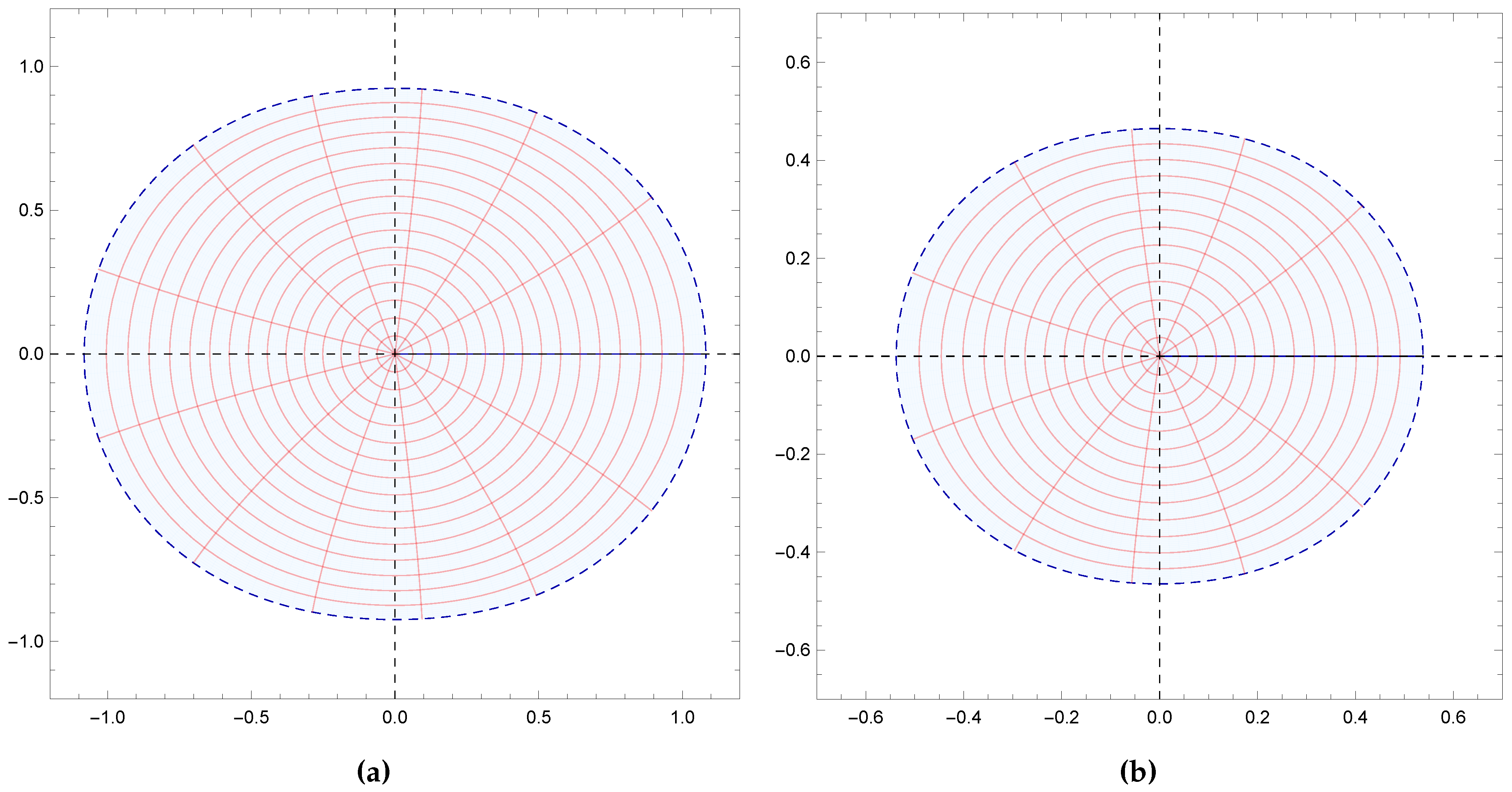
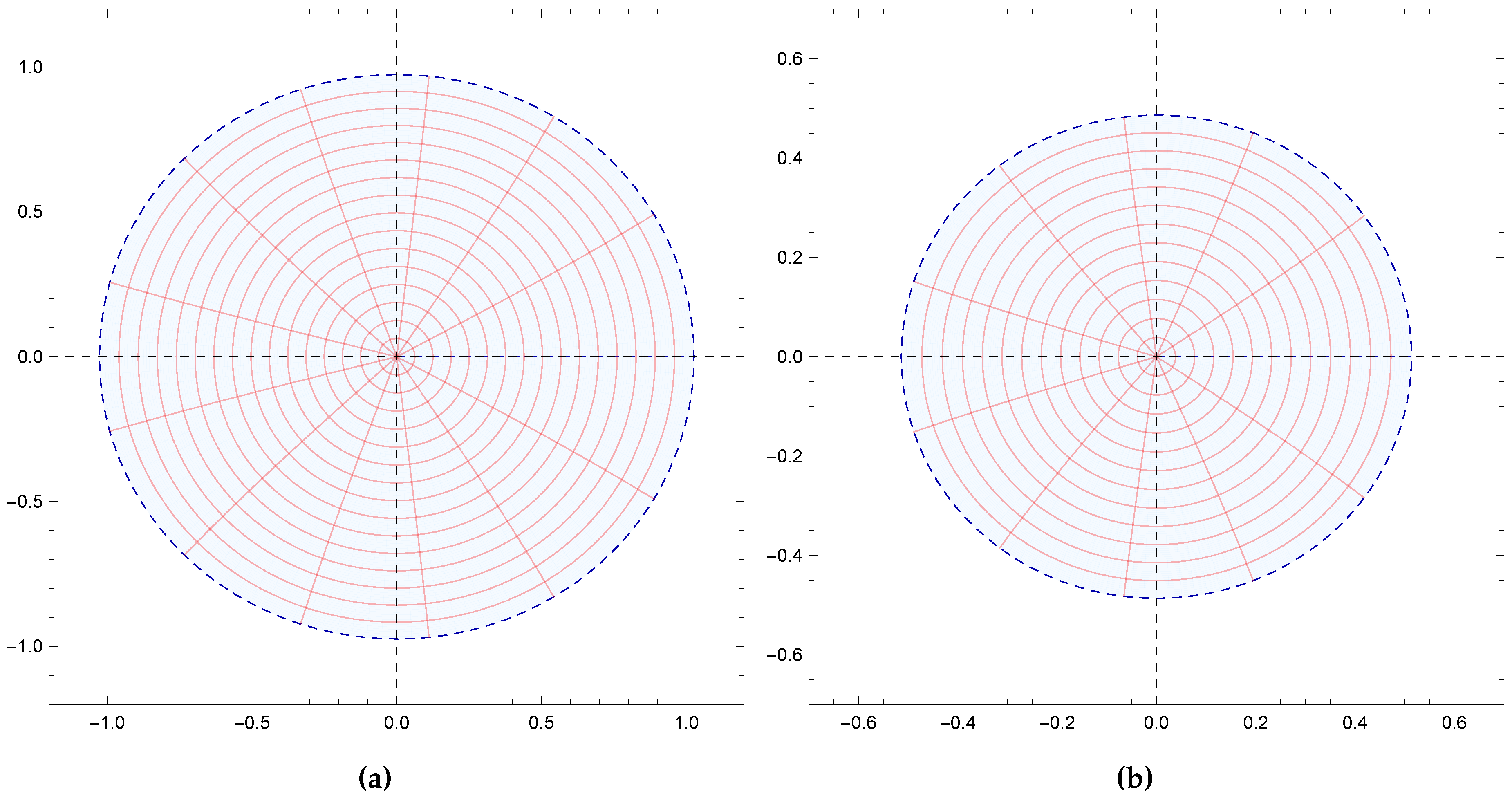
Moreover, the results obtained were also supported by graphical representations generated using Mathematica 12.0. These images effectively depicted the fulfillment of conditions derived from the results, demonstrating the corresponding geometric properties of ${\mathcal{T}}_{\nu }$. Specifically, Figure 1a and Figure 1b demonstrate the starlikeness of ${\mathcal{T}}_{\nu }$ on $\mathbb{D}$ and ${\mathbb{D}}_{{\displaystyle \frac{1}{2}}}$, respectively. 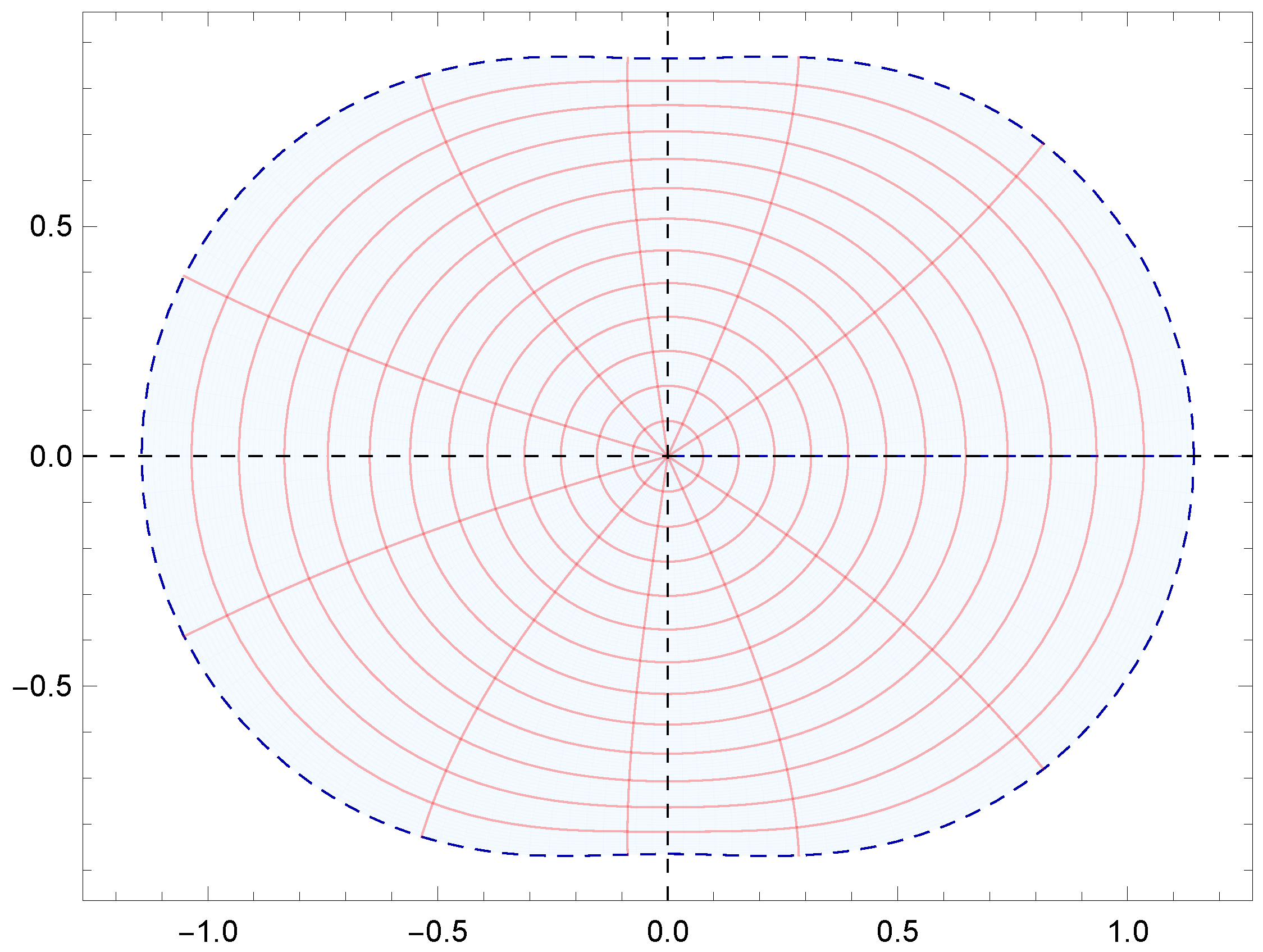Figure 2 showcases the k-starlikeness of ${\mathcal{T}}_{\nu }$ on $\mathbb{D}$. 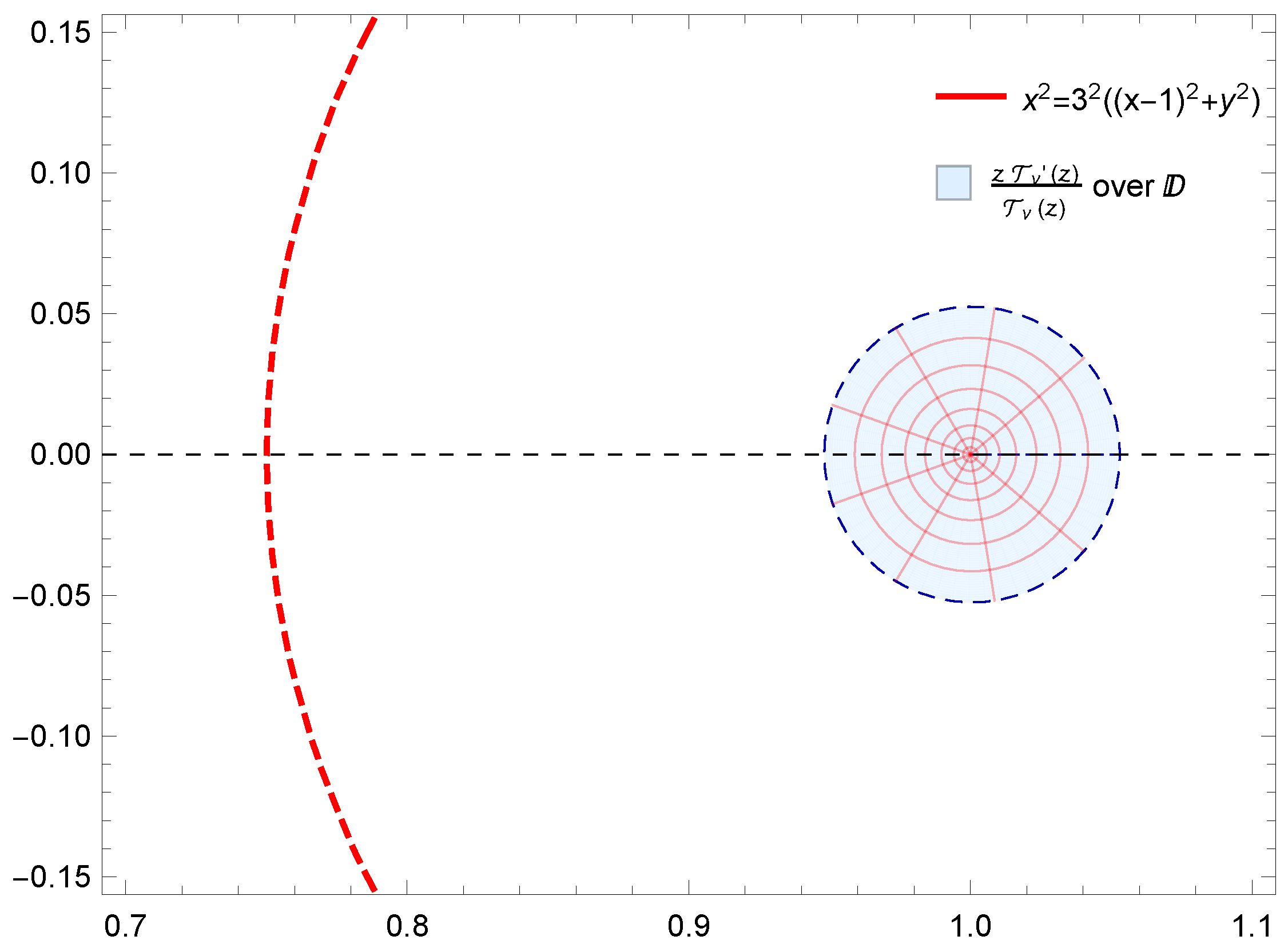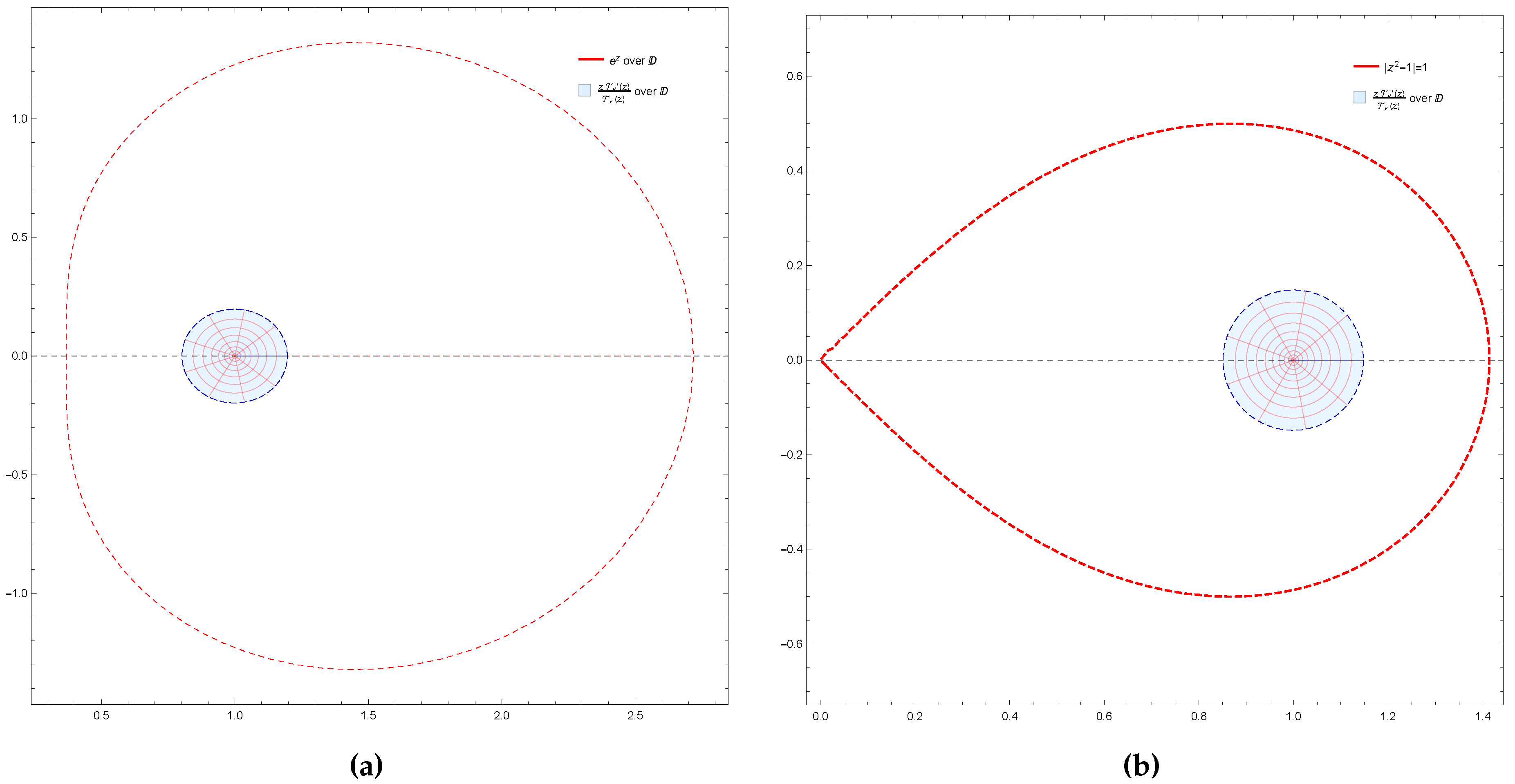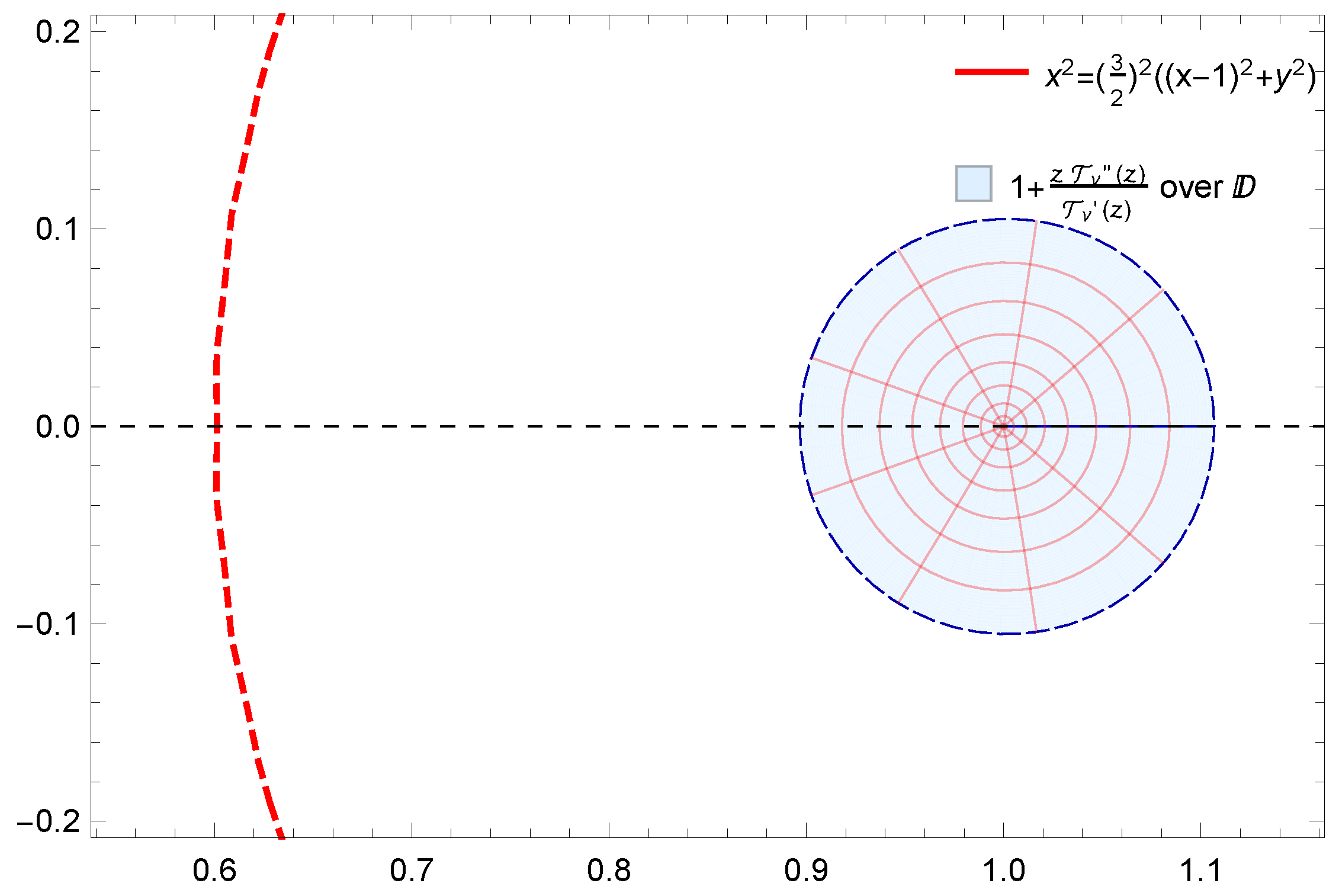Moreover, Figure 3a and Figure 3b exhibit the starlikeness of ${\mathcal{T}}_{\nu }$ associated with the exponential function and the Bernoulli lemniscate on $\mathbb{D}$, respectively. The pre-starlikeness of ${\mathcal{T}}_{\nu }$ can be observed in Figure 4. Furthermore, Figure 5a and Figure 5b illustrate the convexity of ${\mathcal{T}}_{\nu }$ on $\mathbb{D}$ and ${\mathbb{D}}_{{\displaystyle \frac{1}{2}}}$, respectively. Figure 6 presents the k-uniform convexity of ${\mathcal{T}}_{\nu }$ on $\mathbb{D}$. Additionally, Figure 7a and Figure 7b display the convexity of ${\mathcal{T}}_{\nu }$ associated with the exponential function and the Bernoulli lemniscate on $\mathbb{D}$, respectively. These graphical representations provided a comprehensive visualization of the studied properties.

References

- Baricz, Á.; Ponnusamy, S. Starlikeness and convexity of generalized Bessel functions. Integral Transforms and Special Functions 2010, 21, 641–653. [Google Scholar] [CrossRef]
- Prajapat, J.K. Certain geometric properties of normalized Bessel functions. Applied mathematics letters 2011, 24, 2133–2139. [Google Scholar] [CrossRef]
- Mondal, S.R.; Swaminathan, A. Geometric Properties of Generalized Bessel Functions. Bulletin of the Malaysian Mathematical Sciences Society 2012, 35. [Google Scholar]
- Baricz, Á.; Szász, R. Close-to-convexity of some special functions and their derivatives. Bulletin of the Malaysian Mathematical Sciences Society 2016, 39, 427–437. [Google Scholar] [CrossRef]
- Aktaş, İ.; Baricz, Á.; Orhan, H. Bounds for radii of starlikeness and convexity of some special functions. Turkish Journal of Mathematics 2018, 42, 211–226. [Google Scholar] [CrossRef]
- Aktaş, İ.; Baricz, Á.; Singh, S. Geometric and monotonic properties of hyper-Bessel functions. The Ramanujan Journal 2020, 51, 275–295. [Google Scholar] [CrossRef]
- Aktaş, İ.; Baricz, Á. Bounds for radii of starlikeness of some q-Bessel functions. Results in Mathematics 2017, 72, 947–963. [Google Scholar] [CrossRef]
- Aktas, I.; Orhan, H. Bounds for radii of convexity of some q-Bessel functions. Bulletin of the Korean Mathematical Society 2020, 57, 355–369. [Google Scholar]
- Arfken, G.; Weber, H.J. Mathematical Methods for Physicists Academic Press. San Diego 1985. [Google Scholar]
- Szegö, G. On an inequality of P. Turán concerning Legendre polynomials. Bull. Amer. Math. Soc. 1948, 54, 401–405. [Google Scholar] [CrossRef]
- Mezo, I.; Baricz, Á. Properties of the Tur∖’anian of modified Bessel functions. arXiv preprint arXiv:1611.00438, 2016; arXiv:1611.00438 2016. [Google Scholar]
- Duren, P.L. Univalent functions; Vol. 259, Grundlehren der mathematischen Wissenschaften [Fundamental Principles of Mathematical Sciences], Springer-Verlag: New York. 1983. [Google Scholar]
- Kanas, S.a.; Wisniowska, A. Conic regions and k-uniform convexity; 1999; Vol. 105, pp. 327–336.
- Goodman, A.W. On uniformly convex functions. Ann. Polon. Math. 1991, 56, 87–92. [Google Scholar] [CrossRef]
- Kanas, S.a.; Wiśniowska, A. Conic domains and starlike functions. Rev. Roumaine Math. Pures Appl. 2000, 45, 647–657. [Google Scholar]
- Ronning, F. Uniformly convex functions and a corresponding class of starlike functions. Proc. Amer. Math. Soc. 1993, 118, 189–196. [Google Scholar] [CrossRef]
- Sokół, J.; Stankiewicz, J. Radius of convexity of some subclasses of strongly starlike functions. Zeszyty Nauk. Politech. Rzeszowskiej Mat 1996, 19, 101–105. [Google Scholar]
- Mendiratta, R.; Nagpal, S.; Ravichandran, V. On a subclass of strongly starlike functions associated with exponential function. Bulletin of the Malaysian Mathematical Sciences Society 2015, 38, 365–386. [Google Scholar] [CrossRef]
- MacGregor, T.H. The radius of univalence of certain analytic functions. Proceedings of the American Mathematical Society 1963, 14, 514–520. [Google Scholar] [CrossRef]
- MacGregor, T.H. A class of univalent functions. Proceedings of the American Mathematical Society 1964, 15, 311–317. [Google Scholar] [CrossRef]
- Mendiratta, R.; Nagpal, S.; Ravichandran, V. On a subclass of strongly starlike functions associated with exponential function. Bull. Malays. Math. Sci. Soc. 2015, 38, 365–386. [Google Scholar] [CrossRef]
- Kanas, S.; Wisniowska, A. Conic domains and starlike functions. Revue Roumaine de Mathématiques Pures et Appliquées 2000, 45, 647–658. [Google Scholar]
- Kanas, S.; Wisniowska, A. Conic regions and k-uniform convexity. Journal of computational and applied mathematics 1999, 105, 327–336. [Google Scholar] [CrossRef]
- Mehrez, K.; Das, S. Logarithmically completely monotonic functions related to the q-gamma function and its applications. Analysis and Mathematical Physics 2022, 12, 65. [Google Scholar] [CrossRef]
- Ruscheweyh, S. Convolutions in geometric function theory; Vol. 83, Séminaire de Mathématiques Supérieures [Seminar on Higher Mathematics], Presses de l’Université de Montréal, Montreal, QC, 1982; p. 168. Fundamental Theories of Physics.
- Sheil-Small, T.; Silverman, H.; Silvia, E. Convolution multipliers and starlike functions. Journal d’Analyse Mathématique 1982, 41, 181–192. [Google Scholar] [CrossRef]