1. Introduction
The theoretical treatment of laminar flow in curved pipes was pioneered by Dean in the late 1920s [
1,
2]. He showed that in addition to a displacement of streamwise flow, a secondary flow also exists, taking the form of two vortices, the so-called Dean vortices. A constant
D, the Dean number, was identified as the key parameter:
where
is the bulk Reynolds number,
a is the pipe radius and
L is the radius of curvature of the curved pipe. Dean [
1] obtained simplified equations of motion for the approximation
, which can be interpreted as
[
2].
Dean [
1] obtained theoretical solutions to the equations for the range
and following this, McConalogue and Srivastava expanded the solutions numerically to
[
3]. In this paper we treat a subsequent study by Greenspan and Schubert [
4,
5], where numerical solutions were extended to
. This extension was done with a FORTRAN 66 code which is available as an Appendix in [
4]. The purpose of our paper is to convert - and thus revive - this code to modern Fortran. The reason for this is twofold: (i) we need the revived code for planned future research and (ii) we want to make this code available to the scientific community for others who may need a fast and efficient code to calculate basic solutions of laminar flow in slightly curved pipes. This flow system can be considered to belong to the class of canonical laminar flows, which remains relevant for both applied and fundamental research. Note that we also cover a later paper, where improved numerical solutions over than same range of
D were published [
6].
The Dean number of 5000 is from [
7], where experiments determined the critical
to be 5000 for
.
On a personal note, I have previous experience writing and running FORTRAN 77 code on an IBM mainframe at JET [
8] during the period 1997-1998. Thus, the task at hand, to convert FORTRAN 66 code, was feasible.
The paper is structured as follows: In
Section 2, we briefly summarise the equations of motion. This is followed by the FORTRAN 66 code revival steps which are detailed in
Section 3; results from the revived code are presented in
Section 4. A brief discussion is presented in
Section 5 and finally we conclude in
Section 6. The paper thus encompasses the complete path from theory through simulations to results and disseminates the accompanying modernised Fortran code.
2. Equations of Motion
The equations of motion, also called the Dean equations, can be written [
3,
4,
5]:
where:
Here, is the non-dimensional stream function for the secondary flow, w is the non-dimensional velocity in the streamwise direction, r is the normalised pipe radius and is the angle centered on the pipe axis.
To derive the Dean equations, it has been assumed that and that the motion is steady (laminar).
In [
3],
w and
were rewritten as Fourier series and the resulting coupled non-linear equations were solved numerically. In contrast, in [
4,
5], the Dean equations were rewritten to a system of second order equations to facilitate solving the equations using finite differences. This finite difference method was improved upon in [
6] by the application of an additional step to ensure "that the final solutions are correct to central-difference accuracy".
3. Code Revival
There were three aspects to the code revival, and they are treated in the three subsections below:
Digitise the scanned document
Convert the FORTRAN 66 code to modern Fortran
Debugging and testing of the code
3.1. Digitisation
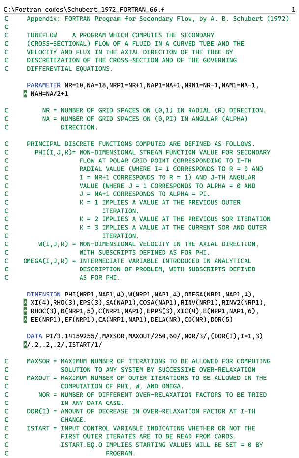
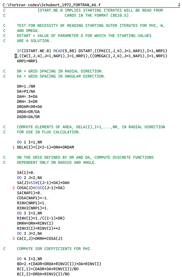
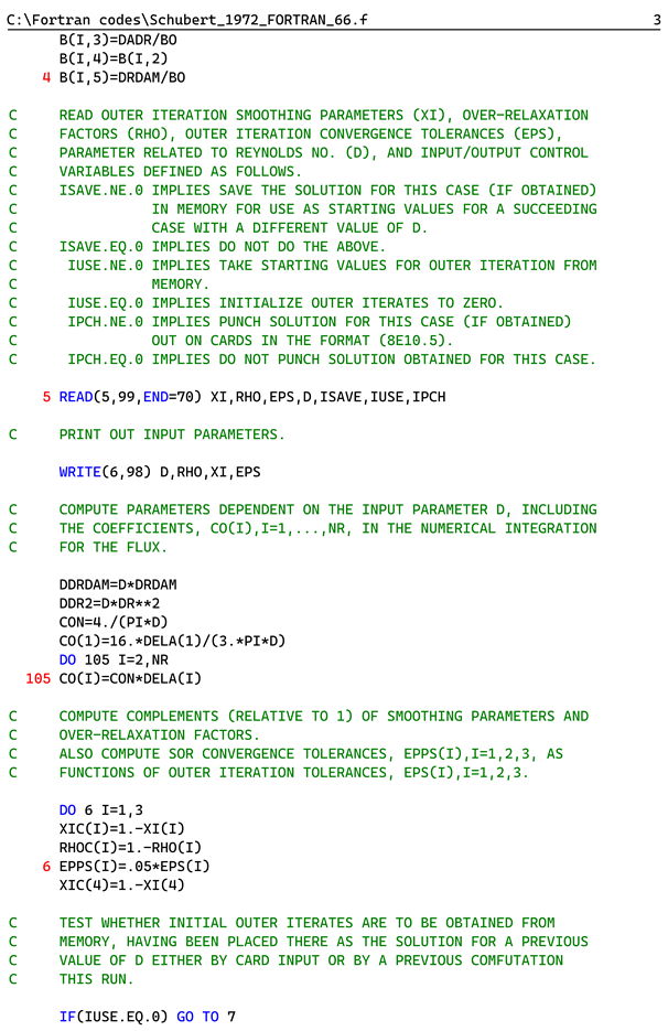
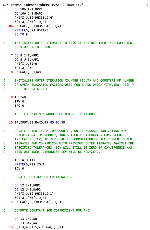
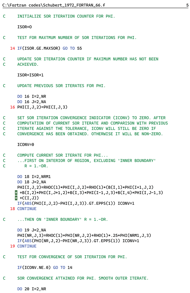
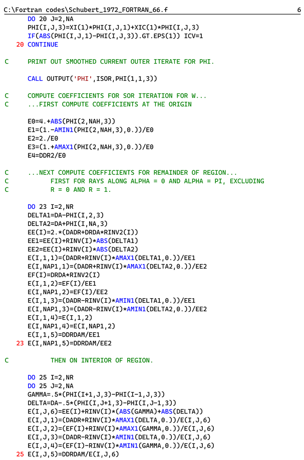
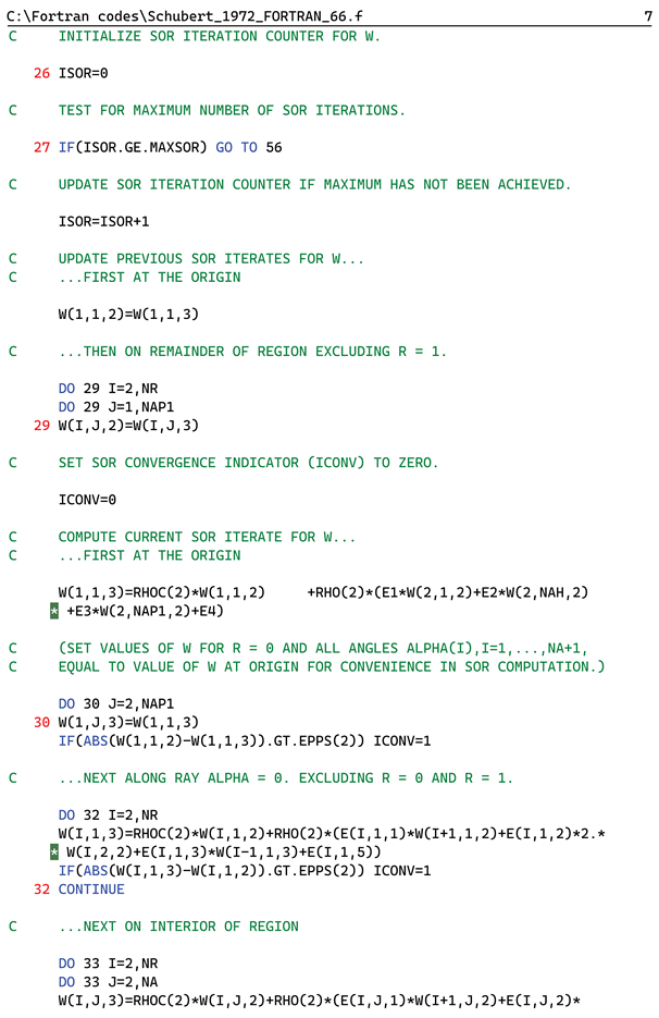
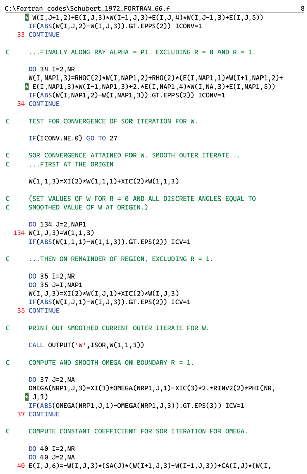
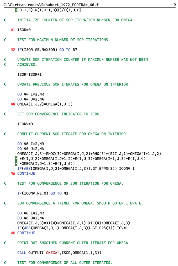
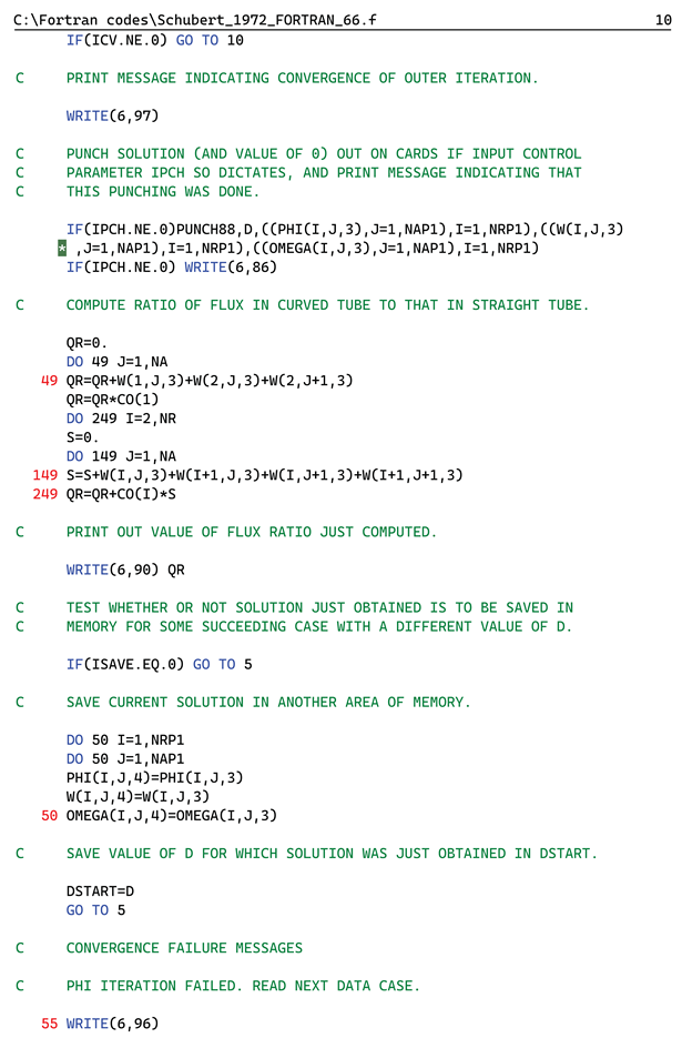
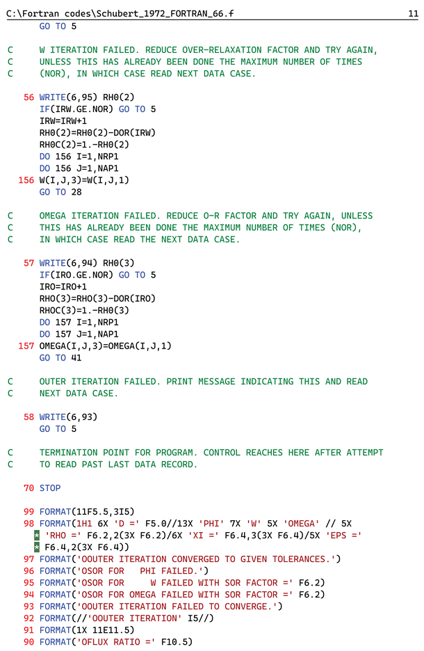
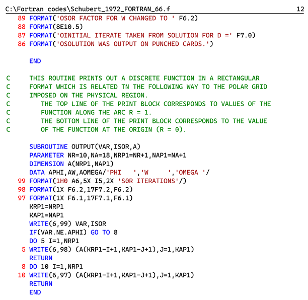
We note that the original FORTRAN 66 code is only available in [
4] and not available in the official journal paper [
5]. As can be seen, the scanned document [
4] has a quite poor quality, making in challenging to perform the optical character recognition (OCR) needed. However, with 12 pages (∼600 lines) of code, it would be very cumbersome to retype the code entirely by hand
We did not attempt to improve the quality of the scanned document before conversion.
Our initial attempts at extracting characters from the scanned document were done using Python with EasyOCR [
9] and PyTesseract [
10]. However, these tools performed poorly on the document.
Our next attempt was with two online converters [
11,
12]. The results were better than for the Python tools, but still with a correct percentage of around 50%.
The best conversion, with a success rate of roughly 80%, was the Amazon Textract tool from Amazon Web Services (AWS) [
13].
In the end, we used the AWS tool to generate the initial digital file and combined it with the output from the two online converters. And finally, a human correction was needed for around 10% of the code.
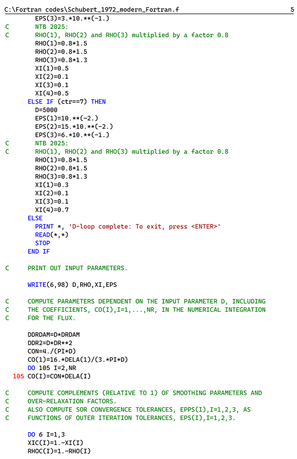
The original FORTRAN 66 code is provided for reference in
Appendix A.
3.2. Conversion
Once the code was available in digital form, the main conversion from FORTRAN 66 to modern Fortran was to replace the Hollerith string and data notation [
14]. To achieve this goal, we also used ChatGPT-4 [
15] to convert the Hollerith commands to modern Fortran. An example of the process can be found in [
16].
3.3. Debugging and Testing
At this stage we had a complete code available, the final step being to debug and test the code.
A laptop with Microsoft Windows 11 [
17] installed was chosen as the hardware/software platform. Microsoft Visual Studio [
18] was installed as the graphical user interface along with the Intel Fortran Compiler (ifx) [
19]. In terms of Fortran versions, ifx uses the latest standards from Fortran 2018 and some Fortran 2023 features. In that sense, we consider the updated code to represent modern Fortran.
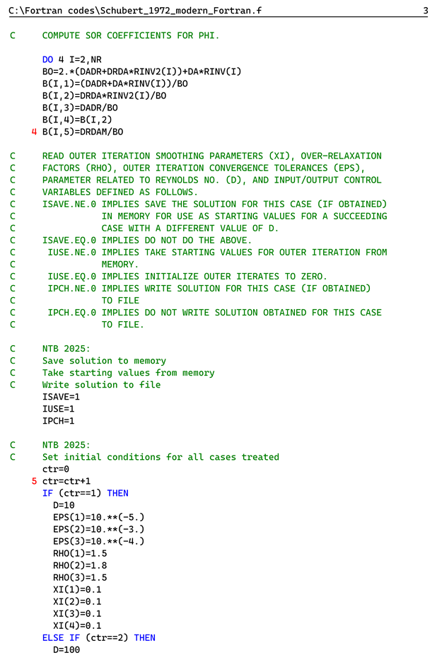
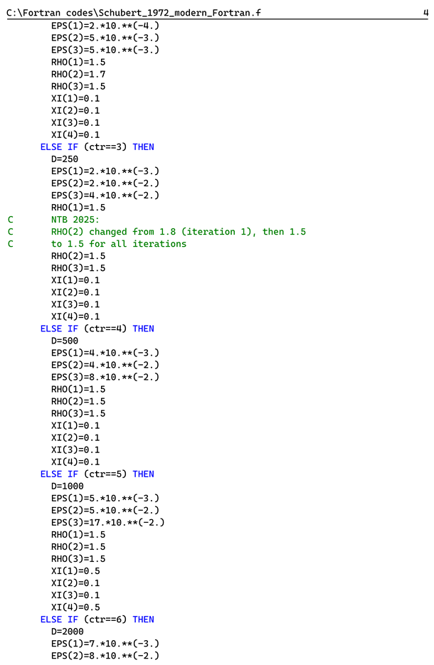
What remained was to compile (build solution) and systematically resolve the errors. Some sections were updated, for example replacing the reading of and writing on punch cards with files. Another major change was to make an IF statement to loop over all
D values analysed in [
4,
5].
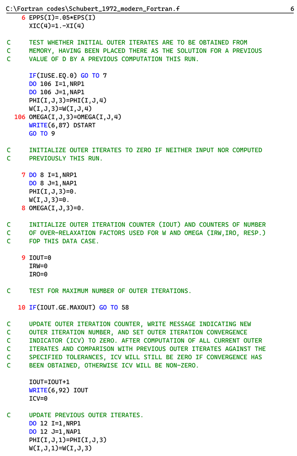
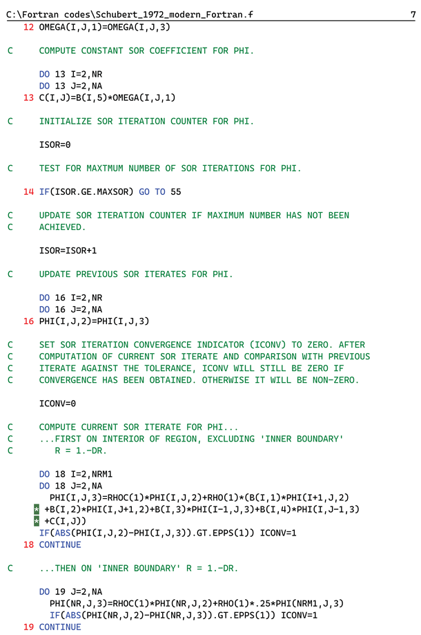
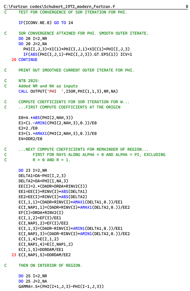
The final result of the steps is the modern Fortran code provided in
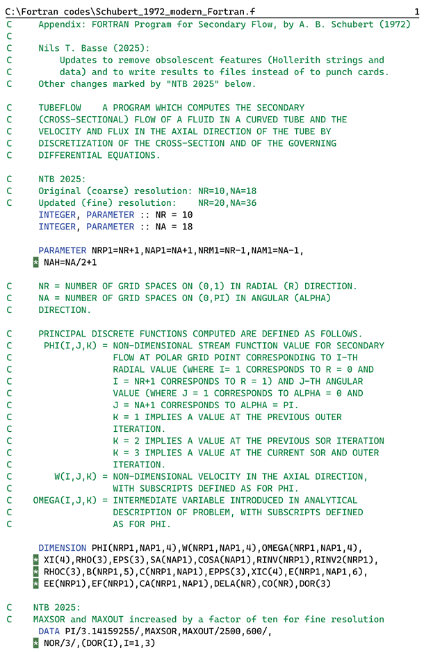
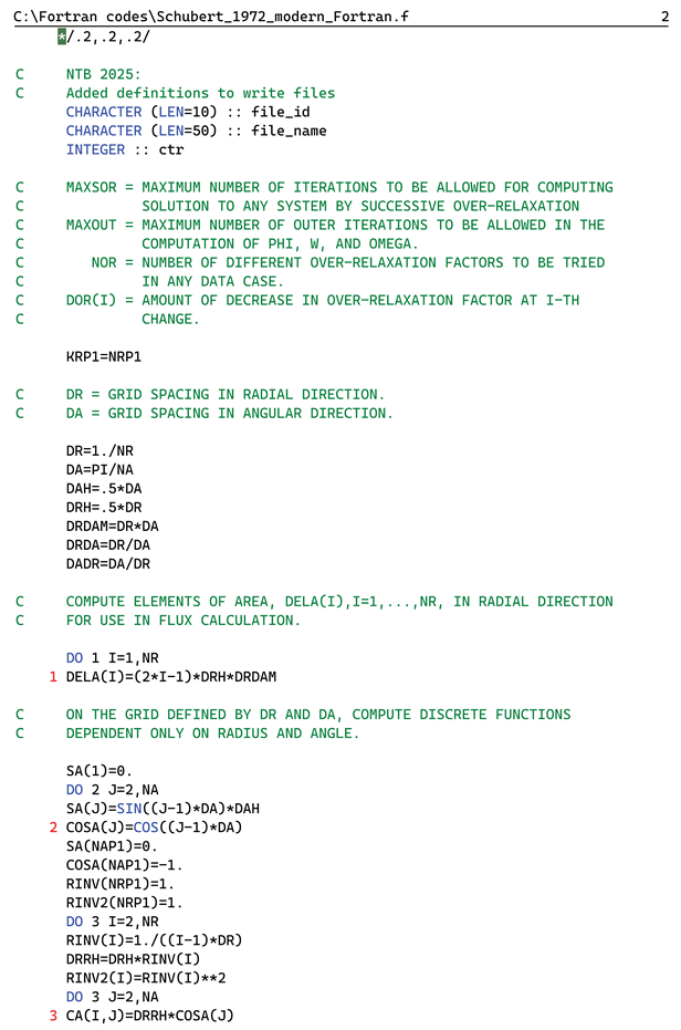
Appendix B. Changes made to the code in addition to the ones mentioned above have been marked by "NTB 2025" in the code to enable an overview of the changes.
The two appendices can be compared to learn what has been deleted from the original FORTRAN 66 code in the modern Fortran code.
4. Results
All postprocessing in this section was done using GNU Octave [
20].
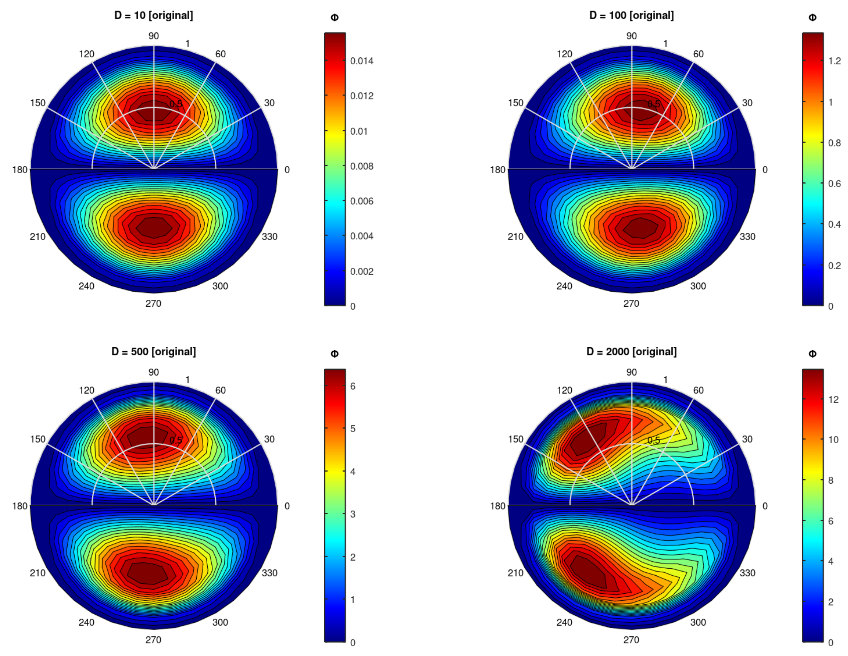
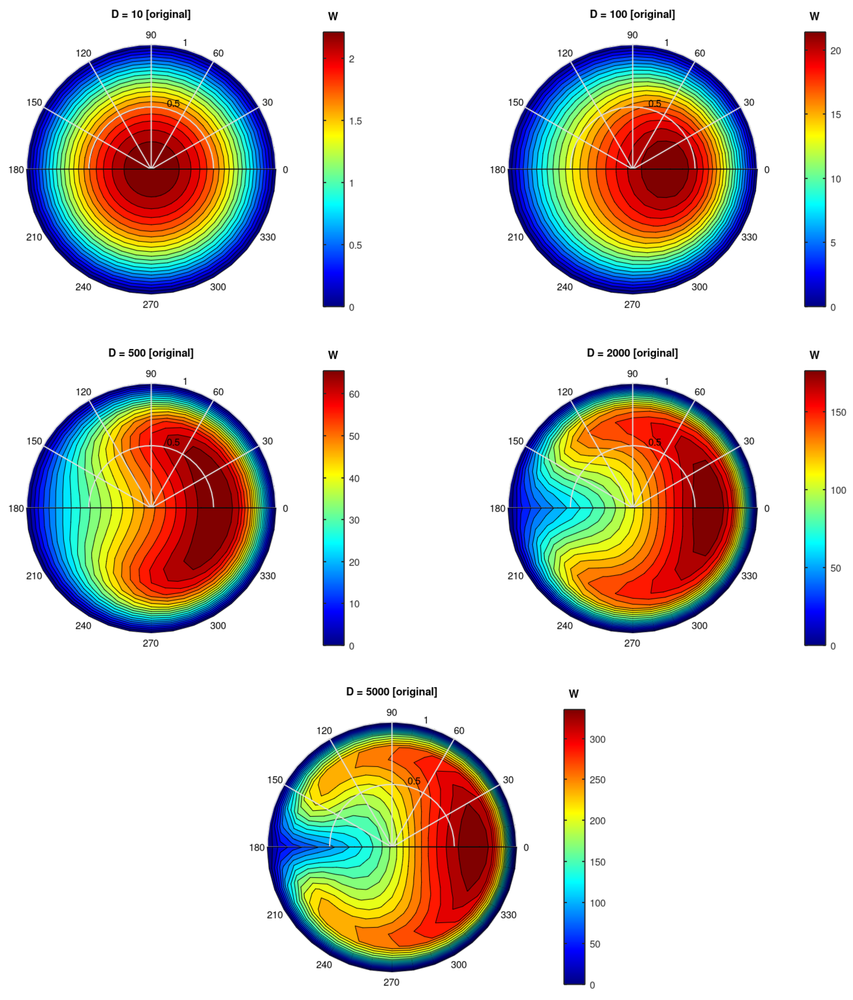
4.1. Evolution of Spatial Structures
We include two figures with contour plots of
and
w,
Figure 1 and
Figure 2, to facilitate a direct comparison to
Figure 3 and 4 in [
5]. Only the upper half of the pipe is calculated by the Fortran code, we mirror this to the lower half for clarity of exposition. Angles
of 0 (180) degrees indicate the outboard (inboard) positions, respectively.
The results match the original results very well, both in position and magnitude.
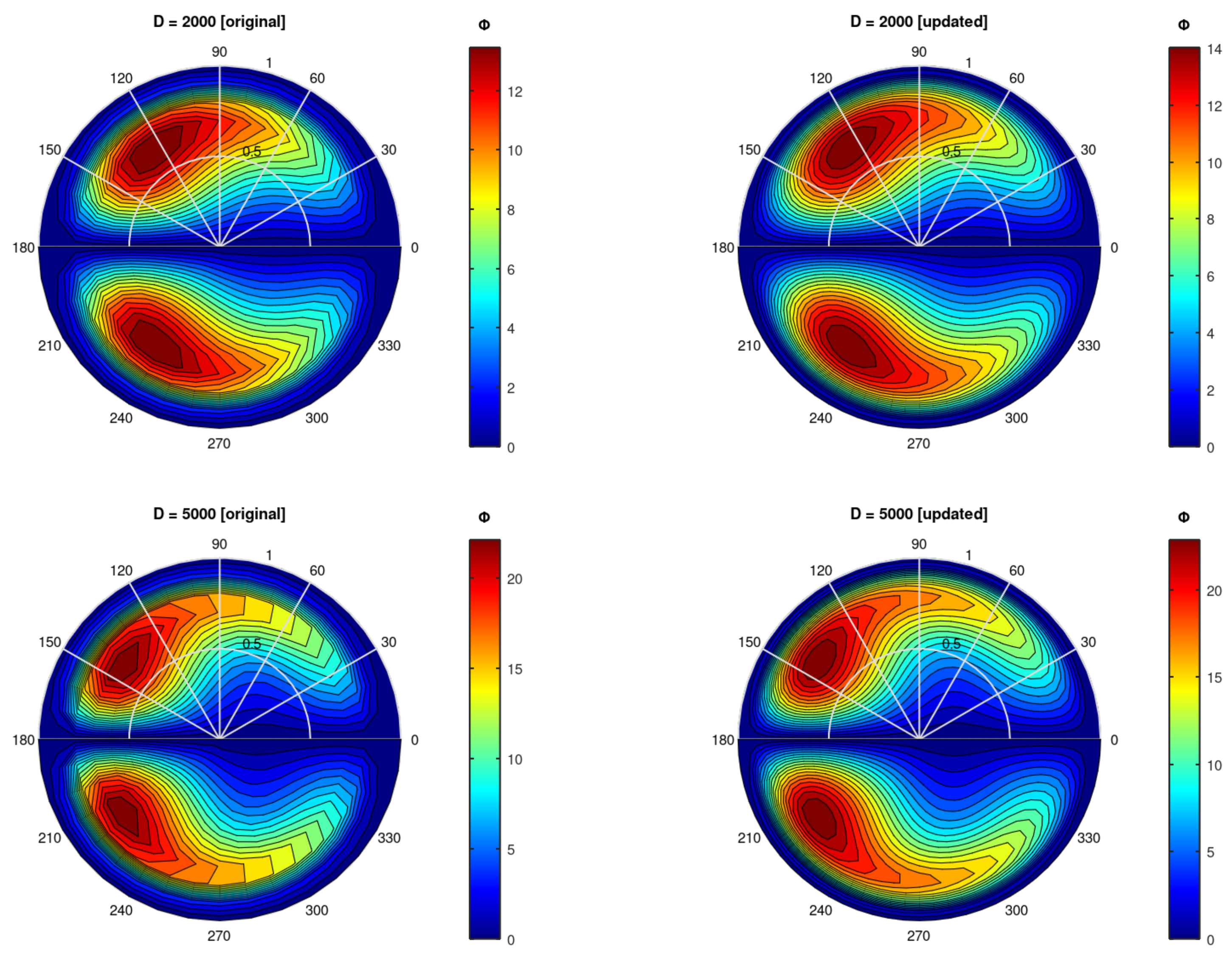
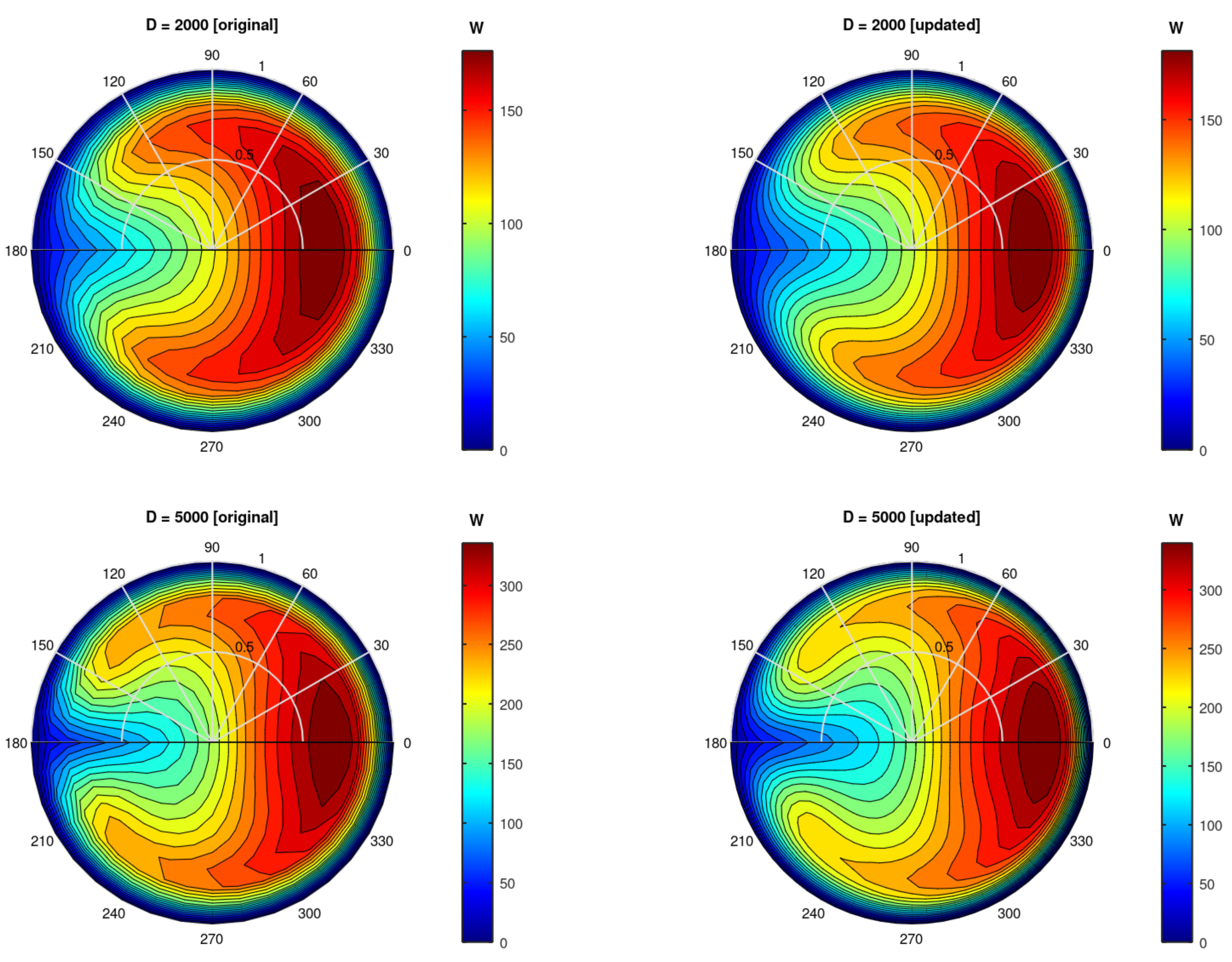
4.2. Grid Resolution Improvement
Having a complete modern Fortran code available enables improvements to e.g. the computational grid resolution. The original resolution was
and
. In the code in
Appendix B, these resolutions are named
NR and
NA, respectively. We updated the code to run with double resolution, both for
r and
. To distinguish the grid resolutions, we call them "original" and "updated".
We compare original and updated contour plots for
and
w in
Figure 3 and
Figure 4. The two largest values of
D are compared; qualitatively, the results are very similar, although the contours of the updated resolution are more smooth than those of the original resolution.
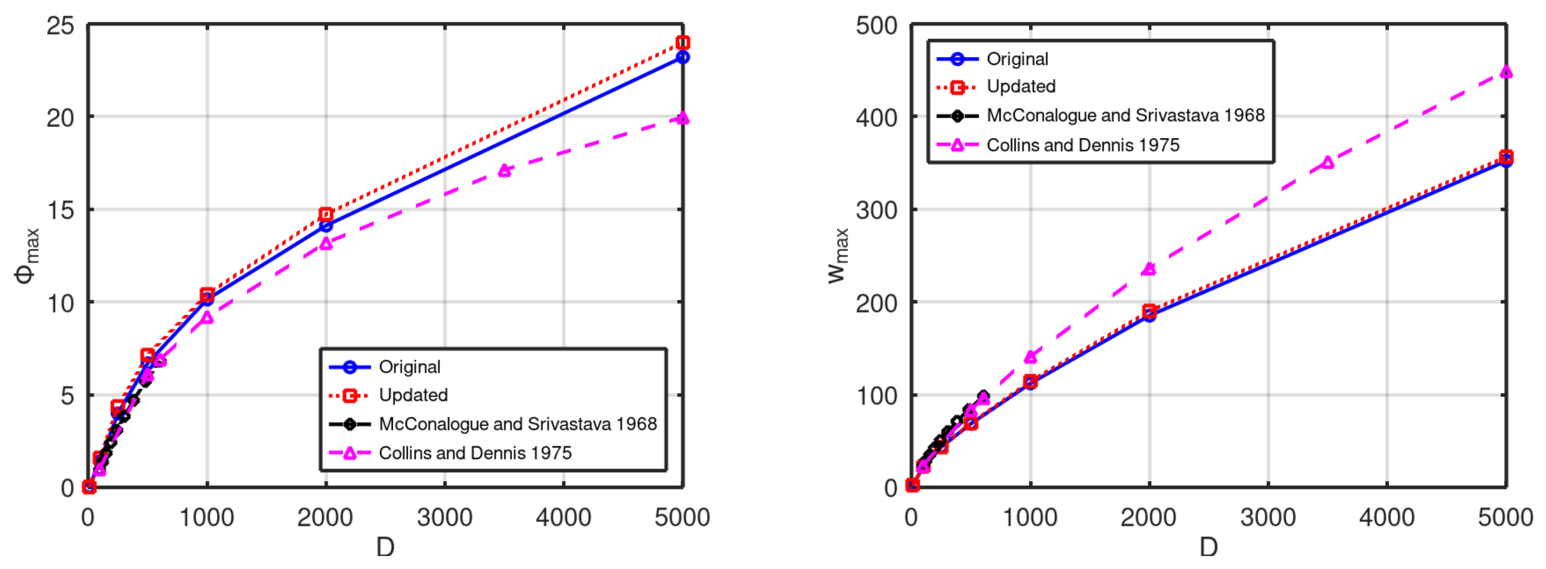
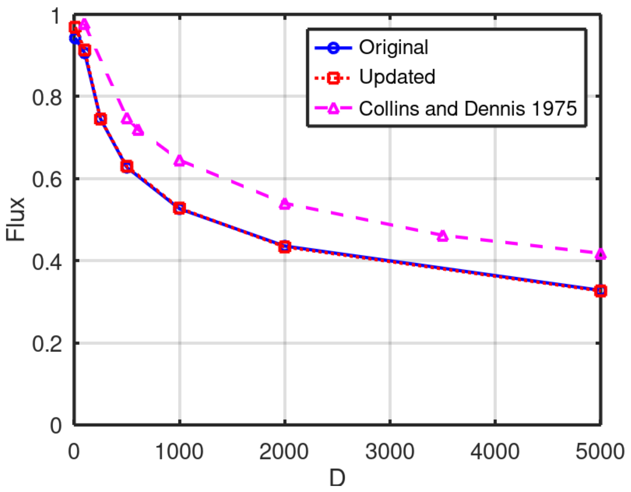
4.3. A Comparison of Scaling Results
We compare results from postprocessing of the running code with literature findings.
In
Figure 5, we present the
D-scaling of the peak values of
and
w, which we name
and
, respectively. Both the original and updated solutions are included, along with results from [
3,
6]. The difference between the original and updated solutions is quite small, but there is a substantial difference between these results and those in [
3,
6]. Measurements (included in [
6]) demonstrate that the values from [
3,
6] are more accurate than our results based on [
4,
5].
An important effect of the secondary flow is the blockage effect, i.e. that it obstructs the streamwise flow. This is also calculated in the Fortran code and shown in
Figure 6 along with values from [
6]. Here, the flux (or flow rate) is normalised to that of a straight pipe. The results are consistent with the
scaling, i.e. the larger flux from [
6] corresponds to a larger
, see the right-hand plot in
Figure 5.
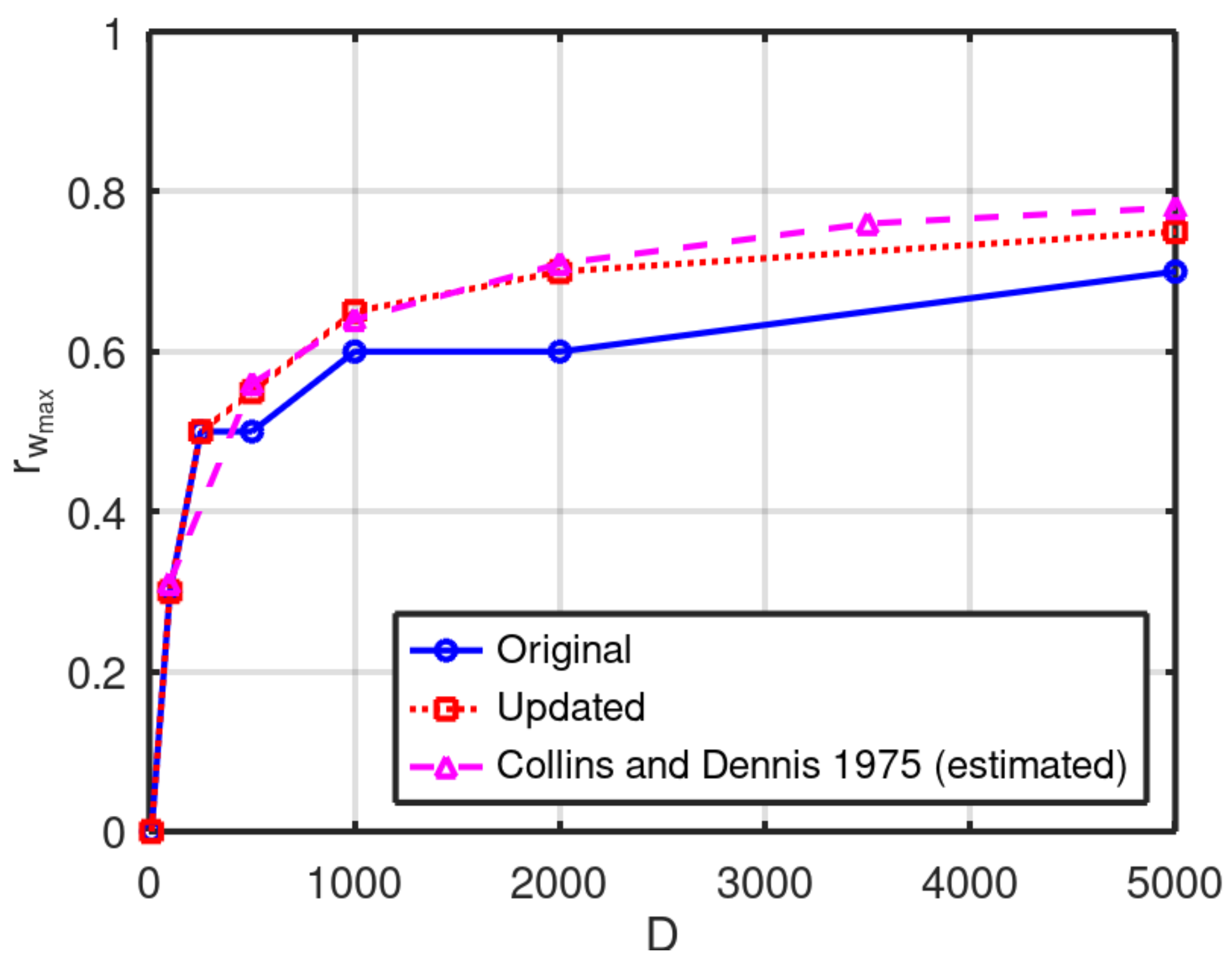
A topic of interest for our future research is how
moves as a function of
D. This is shown in
Figure 7 with values estimated from [
6]. Here, we find a large difference between the original and updated resolution; the updated values are quite close to the results reported in [
6].
5. Discussion
For simulations of both laminar [
21] and transitional (turbulent) [
22] flow, it has become clear that analysis purely based on the Dean number is not valid in general.
For laminar flow, a Dean number based simulation analysis is valid for pipe curvatures
and Dean numbers
[
21]. However, for measurements, the detectable limit is in the vicinity of
[
23].
For the case we treat with slightly curved pipes, the transition to turbulence is subcritical, which is the same as for straight pipes [
22]. From experimental investigations with higher curvature [
24], it is interesting to note the persistence of structures in turbulent flow similar to those identified in laminar flow. Perhaps the laminar flow structures form a skeleton/seed which turbulence builds on?
6. Conclusions
In this paper, we have presented a case study on how to revive older code (FORTRAN 66) to modern Fortran. This code revival has enabled fast calculations of laminar flow through slightly curved pipes. The basis was [
5], with the original code being provided in [
4], see also
Appendix A. The main steps involved were:
Digitisation of the original document with OCR tools and human corrections
Conversion of the FORTRAN 66 code to modern Fortran
Debugging and testing of the modern Fortran code
After the code was operational, we tested increasing the grid resolution and found that the position of the maximum streamwise velocity as a function of
D was sensitive to this change. The positions determined using the increased grid resolution are in satisfactory agreement with those found in [
6]. However,
,
and the flux found with the revived code deviate substantially with established results [
3,
6], even for the increased grid resolution.
We hope that our work serves as a template and inspiration for other scientists who have a need for bringing older code back to life again. Also, the modern Fortran code in
Appendix B is now available to the scientific community as a fast method to obtain a physical picture of streamwise and secondary flow in curved pipes. Finally, the results may serve educational purposes as a toy model of a canonical laminar flow.
The term computational fluid dynamics (CFD) for numerical flow solutions was introduced in 1972 [
25], and the research covered in this paper can indeed be termed CFD, although this nomenclature was not used. An advantage of these early CFD simulations is that they are numerically efficient and thus run extremely fast on modern hardware/software architectures. Therefore, they remain useful as classical solutions which form a foundation for future research. In that spirit, we consider our activities as "numerical archaeology", although this phrase is already in use - albeit with another connotation [
26].
We plan to use the code in the future to facilitate interdisciplinary work on fluids and plasmas which was initiated in [
27].
Funding
This research received no external funding.
Data Availability Statement
The data presented in this paper can be generated by using the modernised Fortran code in
Appendix B.
Acknowledgments
We thank Eurythmics for inspiring the paper title.
Conflicts of Interest
The author declares no conflict of interest.
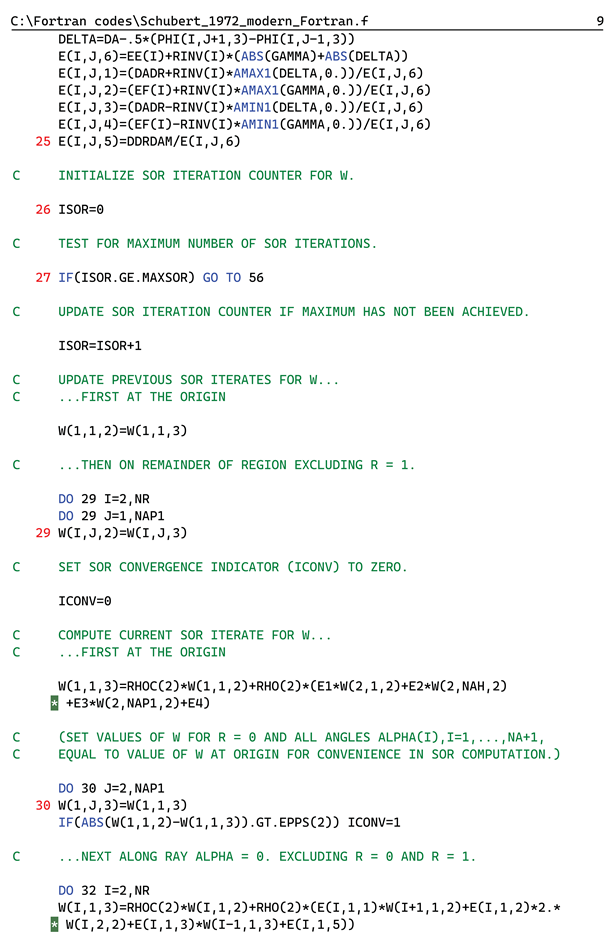
Appendix A. Original FORTRAN 66 Code
For reference, this appendix includes the original FORTRAN 66 code written by A.B.Schubert in 1972 [
4].
This code cannot be compiled and run directly, one reason being that physical punch cards are required.
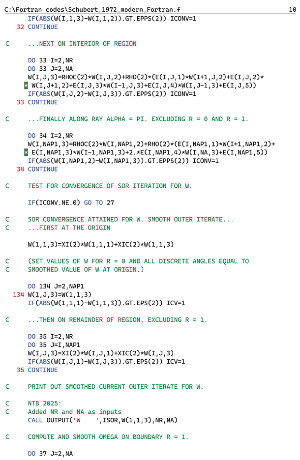
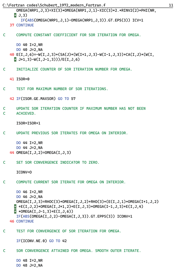
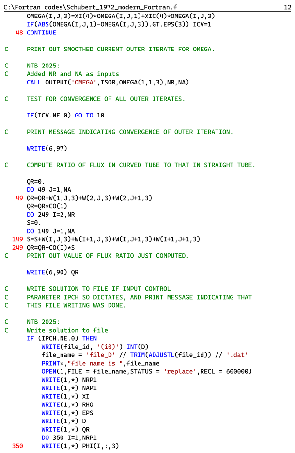
Appendix B. Modernised Fortran Code
This appendix includes the modernised Fortran version of the original FORTRAN 66 code written by A.B.Schubert in 1972 [
4].
Compiling and running the solution creates a separate file for each value of D.
References
- Dean, W.R. Note on the motion of fluid in a curved pipe. Phil. Mag. 1927, 4, 208–223. [Google Scholar] [CrossRef]
- Dean, W.R. The stream-line motion of fluid in a curved pipe. Phil. Mag. 1928, 5, 673–695. [Google Scholar] [CrossRef]
- McConalogue, D.J.; Srivastava, R.S. Motion of fluid in a curved tube. Proc. Roy. Soc. A. 1968, 307, 37–53. [Google Scholar]
- Greenspan, D; Schubert, A.B. Secondary flow in a curved tube. University of Wisconsin, Computer Sciences Department, Technical Report #155 1972. Available online: https://minds.wisconsin.edu/handle/1793/57756.
- Greenspan, D. Secondary flow in a curved tube. J. Fluid Mech. 1973, 57, 167–176. [Google Scholar] [CrossRef]
- Collins, W.M.; Dennis, S.C.R. The steady motion of a viscous fluid in a curved tube. Quart. J. Mech. Appl. Math. 1975, 28, 133–156. [Google Scholar] [CrossRef]
- Taylor, G.I. The criterion for turbulence in curved pipes. Proc. Roy. Soc. A. 1929, 124, 243–249. [Google Scholar]
- Krom, J.G. The evolution of control and data acquisition at JET. Fus. Eng. Des. 1999, 43, 265–273. [Google Scholar] [CrossRef]
- EasyOCR. Available online: https://pypi.org/project/easyocr/.
- PyTesseract. Available online: https://pypi.org/project/pytesseract/.
- PDF.ai. Available online: https://pdf.ai/tools/ocr-pdf.
- MaxAI.me. Available online: https://www.maxai.me/pdf-tools/pdf-ocr/.
- Amazon Web Services. Available online:; https://aws.amazon.com/.
- Metcalf, M.; Reid, J. Fortran 90/95 Explained; Oxford University Press: Oxford, UK, 1996. [Google Scholar]
- OpenAI.com. Available online: https://chatgpt.com/.
- ChatGPT-4 prompt example. Available online: https://chatgpt.com/share/671ccb3e-7ce0-8006-93ae-3c08828444b4.
- Microsoft Windows 11 Enterprise. Available online: https://www.microsoft.com/en-us/microsoft-365/windows/windows-11-enterprise.
- Microsft Visual Studio 2022. Available online: https://visualstudio.microsoft.com/downloads/.
- Intel oneAPI HPC Toolkit 2024.2. Available online: https://www.intel.com/content/www/us/en/developer/tools/oneapi/hpc-toolkit.html#gs.i3q2al.
- GNU Octave, version 9.2.0. Available online: https://octave.org/.
- Canton, J.; Örlü, R.; Schlatter, P. Characterisation of the steady, laminar incompressible flow in toroidal pipes covering the entire curvature range. International Journal of Heat and Fluid Flow 2017, 66, 95–107. [Google Scholar] [CrossRef]
- Canton, J.; Rinaldi, E.; Örlü, R.; Schlatter, P. Critical point for bifurcation cascades and featureless turbulence. Phys. Rev. Lett. 2020, 124, 014501. [Google Scholar] [CrossRef] [PubMed]
- Snyder, B.; Hammersley, J.R.; Olson, D.E. The axial skew of flow in curved pipes. J. Fluid Mech. 1985, 161, 281–294. [Google Scholar] [CrossRef]
- Kühnen, J.; Holzner, M.; Hof, B.; Kuhlmann, H.C. Experimental investigation of transitional flow in a toroidal pipe. J. Fluid Mech. 2014, 738, 463–491. [Google Scholar] [CrossRef]
- Roache, P.J. Computational Fluid Dynamics; Hermosa Publications: Albuquerque, New Mexico, USA, 1972. [Google Scholar]
- Jones, A.R. Lunnon, H., Rodwell, W., Tatton-Brown, T., Eds.; Numerical archaeology: Gleanings from the 1253 building accounts of Westminster Abbey revisited. In Westminster Part I: The Art, Architecture and Archaeology of the Royal Abbey; Routledge: Abingdon, UK, 2017. [Google Scholar]
- Basse, N.T. The chimera revisited: Wall- and magnetically-bounded turbulent flows. Fluids 2024, 9, 34. [Google Scholar] [CrossRef]
|
Disclaimer/Publisher’s Note: The statements, opinions and data contained in all publications are solely those of the individual author(s) and contributor(s) and not of MDPI and/or the editor(s). MDPI and/or the editor(s) disclaim responsibility for any injury to people or property resulting from any ideas, methods, instructions or products referred to in the content. |
© 2025 by the authors. Licensee MDPI, Basel, Switzerland. This article is an open access article distributed under the terms and conditions of the Creative Commons Attribution (CC BY) license (http://creativecommons.org/licenses/by/4.0/).