
Submitted:
15 November 2024
Posted:
18 November 2024
You are already at the latest version
Abstract
In today’s industrial landscape, controlling energy costs, reducing production times, and meeting stringent environmental and quality standards are increasingly critical objectives. These demands are particularly significant in energy-intensive processes such as welding, where reducing energy costs and minimizing production times while maintaining quality is essential. This paper presents an intelligent sensor-software system for decision support in selecting optimal set-point parameters for the resistance spot welding of steel reinforcement bars, considering constraints on quality, energy consumption, and production time as specified by production managers. The system leverages machine learning models trained on process data to develop dynamic, intelligent heat maps that aid production engineers in selecting robust operational points resilient to potential perturbations. These heat maps visually guide the engineer by indicating real-time working conditions and identifying safe operating zones within the quality and efficiency thresholds defined by production management. The proposed methodology consists of the following phases: (i) identification of accurate models using small datasets, (ii) analysis of model robustness under varying conditions, and (iii) creation of interactive heat maps to visually highlight optimal working areas based on predefined optimization criteria, thereby enhancing decision-making in real-world welding applications.
Keywords:
Energy-sustainable decision
; Resistance spot welding
; Intelligent welding
; Machine learning
; Artificial Intelligence (AI)
1. Introduction
Welding is a fundamental process in manufacturing [1], critical for constructing durable and high-strength structures. With the advent of Industry 4.0, many manufacturing companies have successfully implemented automated systems for monitoring and controlling welding processes, effectively closing the loop from creation to quality control [2,3]. These advancements have leveraged historical data from a variety of processes to develop artificial intelligence (AI) techniques aimed at enhancing productivity and minimizing production costs. Within this context, machine learning (ML) has become an essential tool, enabling the creation of intelligent models that can predict outcomes, define set-points, plan, control, and even identify defects in real time. Despite the growing use of AI in Industry 4.0, sustainability concerns—particularly energy efficiency and environmental impact—remain a secondary consideration [4]. Consequently, many companies still rely on manual or semi-automated welding, highlighting the need to fully automate these processes to achieve both sustainability and productivity gains.
Among the various welding techniques available, resistance spot welding (RSW) is particularly economical and productive for joining steel in reinforced concrete structures, as it forms a strong and durable hidden joint within a short processing time [5]. RSW has therefore become a preferred choice for applications requiring high production rates. However, this process presents significant technical challenges due to the need for precise regulation of parameters such as current, pressure, and time. These challenges are compounded by the high energy demands of RSW, where each weld cycle consumes substantial electricity, impacting both operational costs and environmental sustainability. As energy costs continue to rise, optimizing the energy consumption of welding processes while maintaining productivity and quality standards has become a priority for manufacturers [6].
The goal of this study is to develop an intelligent sensor-software for decision-support that aids in selecting optimal setpoint parameters for the RSW process used in steel reinforcement welding for concrete structures. This system is designed to work within predefined quality, energy consumption, and production time constraints, helping operators identify robust operational points that maintain performance even in the presence of perturbations. To achieve this, the system uses machine learning models trained on historical process data to generate intelligent heat maps. These heat maps provide real-time guidance, showing operators the current operating zone as well as highlighting safe and efficient zones based on quality, energy, and productivity metrics.
The RSW process itself involves applying pressure and electrical current to overlapping steel bars, creating a solid-state bond through localized melting and fusion. In the case of reinforced concrete structures, typical configurations require welding bars of different diameters to ensure joint integrity during transport, placement, and concreting. The welding equipment used in this study, PRAXAIR MPH Digital Pneumatic, allows precise control over parameters such as current intensity, pressure, and weld time, with a maximum output power of 50 kVA. However, parameter optimization is crucial to achieving strong, reliable welds without excessive energy consumption. A primary challenge in RSW automation lies in determining the optimal combination of these parameters to balance quality, cost, and sustainability.
To address this, our approach utilizes a small dataset obtained from experimental welds, as detailed in [7]. We developed machine learning models capable of accurately predicting the ideal set-points based on data-driven analysis, despite the limited dataset size—a common issue in industrial settings where experiments can be costly and time-consuming. The proposed methodology includes rigorous model evaluation to ensure that the ML models remain robust and reliable under varying input conditions.
The contribution of this study is twofold. First, we introduce a machine learning (ML) approach to develop models that accurately estimate optimal welding parameters for steel reinforcement bars, ensuring both structural strength and energy efficiency. Second, we present an intelligent heat map-based visualization system that integrates these models to enabling production engineers to identify stable operating zones based on constraints set by production managers regarding quality, production speed, cycle times, and energy use. These intelligent heat maps provide detailed visual insights, allowing production engineers to select optimal settings that align with current production priorities, such as maximizing weld quality, reducing cycle times, or minimizing energy consumption, while adapting to external factors like energy prices.
The paper is organized as follows: Section 2 presents related works on RSW, challenges with small datasets, and visualization techniques. Section 3 describes the dataset on which this study is based. Section 4 outlines the main issues encountered when working with small datasets, as well as background on ML techniques relevant to this research. Section 5 explains the proposed approach, while Section 6 presents the experimental results and a discussion of these findings. Finally, Section 7 concludes the paper by summarizing the main contributions and suggesting future research directions.
2. Background
2.1. The Resistance Spot Welding Process
Artificial Intelligence (AI) has significantly advanced the understanding and optimization of the Resistance Spot Welding (RSW) process [8,9]. Techniques such as neural networks [3,10] and adaptive neuro-fuzzy inference systems (ANFIS) [9] have been employed to predict weld strength in steel sheets with high accuracy. Additionally, carbon emissions from welding processes have been modeled to assess environmental impacts [11].
The recent surge in manufacturing data has facilitated the application of machine learning (ML) in welding quality prediction. For instance, logistic regression models have been utilized to predict defects in electric resistance welded tubes, yielding satisfactory results and enabling the estimation of safe operating ranges for process variables [12]. Support vector regression has also been applied to predict quality in electron beam welding [13]. Furthermore, feature engineering-based ML approaches have been proposed for quality prediction in RSW of steel sheets, combining engineering and data science perspectives to provide insights into welding data and account for the dynamic nature of RSW due to factors like cooling time and electrode wear [14].
In recent years, there has been a growing interest in integrating AI with sensor data to enhance RSW processes. For example, a study developed a machine learning tool to predict the effect of electrode wear on weld quality, achieving an accuracy of 90% [15]. Another research utilized a convolutional neural network (CNN) combined with a long short-term memory (LSTM) network and an attention mechanism to detect welding quality online, achieving a detection accuracy of 98.5% [16]. Additionally, AI-driven interpretation of ultrasonic data has been explored for real-time quality assessment in RSW, highlighting the potential of adaptive welding using ultrasonic process monitoring backed by AI-based data interpretation [17].
Despite these advancements, the application of AI in the RSW of reinforcement bars (rebar) remains underexplored. Moreover, existing studies primarily focus on predictive modeling and do not incorporate visualization techniques to facilitate sustainable decision-making beyond the outputs of ML models. This gap underscores the need for research that integrates AI-driven predictive models with intuitive visualization tools to support informed and sustainable decisions in RSW processes.
2.2. Challenges of Working with Small Datasets
Automating complex industrial processes, such as resistance spot welding (RSW), often encounters the challenge of limited data availability during initial implementation phases. In many cases, comprehensive process data are scarce, necessitating the acquisition of information through meticulously designed experiments that span the entire operational state space. Typically, these datasets consist of process conditions as inputs and corresponding weld quality parameters as outputs. Machine learning (ML) models can be developed from this data to predict optimal setpoints based on predefined requirements. However, constructing and deploying these models is particularly challenging when relying on experimental datasets, primarily due to their limited size and scope.
The high economic and time costs associated with experimental data collection often result in datasets that are insufficiently large to capture the full spectrum of process variability. This limitation can lead to the development of overfitted models—models that have learned the training data too well and, consequently, fail to generalize to new, unseen conditions [18]. Overfitting is a common issue in models with high complexity, such as deep neural networks with numerous parameters or extensive regression trees, where the model effectively ’memorizes’ the training data rather than learning the underlying patterns.
Conversely, employing less flexible algorithms, such as simple linear regression, may yield models with inadequate accuracy, rendering them unsuitable for capturing the complexities of the process. Therefore, selecting an appropriate algorithm and meticulously tuning its parameters are critical steps in developing accurate ML models, especially when dealing with small datasets [19]. Robustness is a key consideration to ensure that the setpoints derived from these models remain reliable and stable, even in the presence of input perturbations.
Recent studies have explored various strategies to address the challenges associated with small datasets in ML applications. Techniques such as data augmentation, transfer learning, and the use of ensemble methods have been investigated to enhance model performance and generalization capabilities [20]. Additionally, the integration of domain knowledge into the modeling process has been shown to improve the reliability of predictions, particularly in industrial applications where expert insights can compensate for limited data [21].
In summary, effectively managing the constraints of small datasets requires a balanced approach that combines careful algorithm selection, parameter tuning, and the incorporation of domain expertise. Such strategies are essential to develop robust and accurate ML models capable of supporting automation in industrial processes like RSW.
2.3. AI-Driven Visualization Approaches for Decision Support Systems
Decision Support Systems (DSS) have become indispensable tools in complex decision-making processes, particularly with the integration of Artificial Intelligence (AI) models. The rapid advancement and predictive power of AI have led to its widespread adoption across various industries. In industrial contexts, AI models are commonly developed for classification and regression tasks using supervised learning, as well as for clustering unlabeled data to uncover hidden relationships through unsupervised learning. The success of AI applications in multiple fields over recent years has established it as a state-of-the-art technique in numerous contexts.
While much of the recent literature on DSS has focused on developing AI models with high predictive capabilities, the visualization of results remains a critical component. Effective visualization techniques simplify complex data, facilitating decision-making by presenting AI model predictions in an accessible manner. Graphical visualization techniques can obscure the complexity of DSS, enabling users to make decisions more easily and efficiently [22]. Visualizations that offer sufficient guidance emphasize critical information and encourage more rational decisions [23,24,25]. Visual browsing positively impacts item and region discovery, attributed to the ability to quickly analyze large amounts of information in a straightforward manner [26].
Various visualization techniques have been employed to aid decision-making across different contexts, including scatter plots, graph-based interfaces, Venn diagrams, dendrograms, and tree maps [27,28,29,30]. Among these, heat maps are particularly well-known and widely used. Heat maps display data in a two-dimensional grid format, where color intensity represents data magnitude. They are commonly utilized in DSS for data analysis, such as in quality control, to identify areas with high or low data values.
Despite their utility, heat maps have certain limitations. They often offer limited interactivity, as they are typically static images that cannot be easily manipulated or explored—a significant drawback when displaying large amounts of information. Additionally, heat maps are susceptible to visual biases, and comparing values across different parts of the visualization can be challenging, making it difficult to identify patterns and trends in the data.
Recent advancements aim to address these limitations by enhancing heat map visualization techniques. One approach involves adding interactivity features such as zooming, panning, and tooltips, allowing users to explore data more thoroughly and identify specific data points or trends. For instance, interactive cluster heat maps have been developed to visualize and explore multidimensional metabolomic data [31], and spatial analyses of financial development’s effect on the ecological footprint of Belt and Road Initiative countries have utilized heat maps with labels [32]. Interactive heat maps have also been employed as analysis and exploration tools for epigenomic data [33] and for residential energy consumption studies [34]. In recent years, tools have emerged to facilitate the creation of interactive heat maps, successfully applied in fields such as biology, cancer research, COVID-19 studies, single-cell analysis, and immunology [35,36]. While three-dimensional (3D) heat maps exist, they are generally not recommended for data representation due to potential interpretative challenges [37].
Furthermore, integrating machine learning algorithms into heat map generation has been proposed to create more informative visualizations. These advanced heat maps analyze data to highlight patterns and trends that may be difficult to detect with standard techniques [38]. By combining AI with enhanced visualization methods, DSS can provide more effective and user-friendly tools for complex decision-making processes.
3. The RSW Process Dataset
This study utilizes a dataset on the strength of Resistance Spot Welding (RSW), created through controlled welding experiments and described in detail by Ferreiro-Cabello et al. [7]. The following lines summarize the process of creating the dataset and expand on its main features, incorporating additional context and methodology details.
The dataset includes welding tests on rebar of structural steel B500-S, specifically in diameters commonly used in reinforced concrete structures: 8, 10, 12, and 16 mm. These diameters were selected to represent a range of joint thicknesses between 16 mm and 32 mm, as shown in Table 1. For each combination, the test configuration consisted of welding three bars of diameter B to one of diameter A, as illustrated in Figure 1. This configuration ensured that the dataset would include the most frequently used joint dimensions in the production of electro-welded meshes.
The welding experiments were conducted using a PRAXAIR MPH Digital Pneumatic welder, equipped with a maximum power output of 50 kVA. This equipment enabled precise adjustments of key welding parameters, including time (t), current intensity (I), and pressure (p). Welding time was controlled by a digital system, which allowed for cycles of up to 2 seconds, split into different active time percentages to match the joint thickness. Three discrete values of pressure (5, 6, and 7 bars) were used, and current intensity varied from 40% to 80% of the maximum power, as shown in Figure 2.
A total of 2160 welds were performed, corresponding to 360 combinations of t-I-p for each joint thickness. For each parameter combination, two sets of six welded bars were prepared to assess both strength and deformation characteristics. The welding parameter commands are shown in Table 2.
To evaluate joint deformation, the contact area thickness was measured after welding. This measurement was conducted using a Palmer micrometer to ensure non-destructive sampling accuracy. The deformation (D) was calculated as:
where represents the individual thickness measurements. An acceptable weld was defined by minimum values of N and , filtering out any outliers due to test errors.
In addition to thickness measurements, weld strength was tested using destructive shear () and tensile () tests with a Servosis ME-420/20 machine. For each combination, the mean values of shear () and tensile () strength were calculated. The combined strength (S) was computed using:
as illustrated in Figure 1. This comprehensive testing provided reliable data on joint performance across various conditions.
Finally, the dataset consists of five input variables (diameters A and B, t, I, and p) and two output variables (S and D). Extreme outliers were removed, resulting in a final dataset of 298 rows, each representing a unique welding condition.
Figure 3 shows the distribution of joint thickness across experiments, confirming the dataset’s balanced coverage for different joint thicknesses. This balance ensures that the dataset represents a diverse range of welding conditions applicable to industrial RSW processes.
4. Machine Learning-Based Strategy for Small Datasets
The primary task in developing a machine learning (ML)-based decision support system involves testing various models and optimizing their hyperparameters. When working with large datasets and numerous hyperparameters, it is common practice to limit the number of models tested and use grid search for hyperparameter optimization due to the substantial computational cost of each experiment.
In this study, however, the dataset is relatively small (298 rows with five input variables and two target variables). This smaller dataset size has three key implications:
- There is an elevated risk of overfitting.
- The limited dataset size necessitates additional experimental trials.
- Feature selection is unnecessary, as there are only five input variables.
To mitigate the risk of overfitting in training, we employ a nested cross-validation approach. Given the small dataset size, this method is repeated multiple times to enhance the robustness of the results. Additionally, hyperparameter optimization is performed using Bayesian optimization rather than the more conventional grid search, which improves efficiency and allows for more refined parameter tuning.
Beyond traditional models like random forest (RF) and multilayer perceptron (MLP), we also evaluate a powerful AutoML tool, Autogluon, to further streamline and enhance the modeling process.
4.1. Bayesian Optimization
Bayesian optimization [39] is a popular algorithm for hyperparameter optimization in machine learning models. While alternative methods like evolutionary algorithms [40] and particle swarm optimization [41] exist, they are typically more computationally expensive and often require numerous evaluations.
In Bayesian optimization, a probabilistic model of the objective function is iteratively updated to guide the selection of hyperparameters. This process involves evaluating the model with selected hyperparameters, updating the probabilistic model based on performance, and repeating until an optimal set of hyperparameters is identified. By leveraging past iterations, Bayesian optimization focuses the search on promising regions of the hyperparameter space.
Compared to standard methods like grid and random search, Bayesian optimization provides a more efficient exploration of the hyperparameter space. Unlike grid search, which examines a fixed set of points and may miss key regions, Bayesian optimization uses its probabilistic model to adaptively explore high-potential areas, even in the presence of non-convex or noisy objective functions. This adaptability helps it avoid local optima and manage evaluation noise more effectively. However, since Bayesian optimization relies on iterative learning from previous evaluations, it tends to have higher computational costs per iteration.
4.2. Nested Cross-Validation
Cross-validation (CV) is essential when developing machine learning models, as it provides a reliable estimate of model performance on unseen data and helps mitigate overfitting. The core idea of cross-validation is to split the dataset into training and testing sets multiple times. The model is trained on each training set and evaluated on the corresponding testing set. Repeating this process across different data splits yields a more robust estimate of the model’s performance. The most common method, k-fold cross-validation, divides the dataset into k equally-sized folds. The model is trained on folds and tested on the remaining fold. This process is repeated k times, so each fold is used once for testing.
The development of AI/ML systems is prone to errors, especially related to model biases and dataset shifts [42]. Model biases often stem from improper training procedures, leading to skewed inference results. Dataset shifts, on the other hand, arise from mismatches between training and testing data distributions. These issues are particularly challenging with small datasets, where the limited data volume amplifies the risk of overfitting and makes mistakes more likely.
Nested cross-validation is a technique designed to evaluate both the generalization error of a machine learning model and its hyperparameters. It is an extension of the k-fold cross-validation approach and is particularly beneficial when working with small datasets and models with numerous hyperparameters to tune [43]. Algorithm 1 presents a pseudo-code version of the process.
The key concept in nested cross-validation is the use of two nested loops of cross-validation:
- Outer loop: The outer loop splits the data into training and testing sets, similar to standard cross-validation. However, rather than using the same hyperparameters across all folds, a unique set of hyperparameters is selected for each fold.
- Inner loop: The inner loop is dedicated to hyperparameter selection. It performs cross-validation on the training set to assess the model’s performance with various hyperparameter configurations. The set of hyperparameters that performs best in the inner loop is then used to train the model on the full training set in the outer loop.
| Algorithm 1 Pseudo-code for nested cross-validation |
|
5. Methodology
The proposed methodology involves a series of steps designed to optimize the machine learning (ML) models, ensure their robustness, and facilitate sustainable decision-making. The steps are as follows:
- Selection of ML algorithms: Choosing the most appropriate algorithms based on the nature of the problem and the limited dataset size.
- Model training and evaluation: Implementing nested cross-validation combined with Bayesian optimization for hyperparameter tuning to enhance model performance and prevent overfitting.
- Robustness analysis: Assessing model robustness to ensure reliable performance across various data conditions.
- Heat map generation: Developing interactive heat maps to support sustainable decision-making by visualizing optimal operational regions.
5.1. Selection of the ML Algorithms
The main goal was to develop machine learning (ML) models capable of making robust and accurate predictions of S (strength) in Newtons (N) and D (deformation) as a percentage (%). As described in Section 3, the dataset consists of 298 experimental cases with five input variables representing each test configuration: A-B-t-I-p, along with two output target variables: S (strength) and D (deformation).
To enhance model training, the distribution of the target variables was improved by applying a square root transformation. This adjustment aimed to reduce skewness and improve the stability of the predictions. Finally, the entire dataset was normalized to ensure uniformity in the input scale across all variables.
The following algorithms were selected for experimentation due to their suitability for small datasets: ridge regression (Ridge), kernel ridge regression (KRidge), decision tree regressor (DTR), random forest regressor (RF), support vector regression (SVR), and multi-layer perceptron (MLP). All of these algorithms are available in the scikit-learn Python library and are well-suited for the dataset size and structure. Table 3 summarizes the hyperparameter optimization ranges for each model.
In addition to these established ML models, the AutoGluon AutoML tool was also included in the experiments to explore potential performance gains through automated model selection and tuning. Other algorithms, such as Lasso regression, K-Nearest Neighbors regression, and Gaussian process regression, were excluded from the final experiments due to suboptimal performance with this dataset.
5.2. Training and Evaluation
Once the models were selected, we proceeded with their training and evaluation. Given the small dataset size, which increases the risk of overfitting but allows for multiple experimental trials, we incorporated two advanced techniques: Bayesian optimization and nested cross-validation. Although widely recognized, these techniques are not typically part of standard AI model development, where simpler approaches such as grid search and basic cross-validation are more common.
Bayesian optimization was particularly suited to this problem due to its balance between performance and computational efficiency, making it ideal for the dataset size and the need for a robust cross-validation scheme.
For model validation, we employed a repeated k-fold nested cross-validation to ensure both accurate hyperparameter tuning and reliable performance estimation. Specifically, we performed a 10-times repeated 10-fold nested cross-validation. In each repetition, the outer loop ran 10 times, creating 10 unique test sets. For each iteration of the outer loop (i.e., with a fixed test set), we conducted a 9-fold cross-validation within the inner loop, using Bayesian optimization with 200 iterations to fine-tune the hyperparameters. In the inner loop, the non-test data was divided into 9 parts: 8 for training and 1 for validation. This inner cross-validation process was repeated 9 times, and the best hyperparameters identified were used to retrain the model on the combined training and validation sets before evaluating it on the test set. Predictions on the test set were stored for subsequent analysis. Figure 4 illustrates an example of the inner loop in one iteration of the outer loop. This process resulted in a total of 100 different training, validation, and testing partitions.
Overall, this nested cross-validation process was repeated 10 times, leading to 900 executions of the inner loop for hyperparameter optimization and 100 executions of the outer loop. The final predictive performance was reported as the mean Root Mean Square Error (RMSE) obtained from the 100 outer loop iterations.
5.3. Robustness Analysis
Robustness analysis is crucial in machine learning (ML) applications within the industrial sector, as it ensures models are reliable, accurate, and compliant, thereby mitigating risks associated with incorrect predictions. Sensitivity analysis serves as a key tool in assessing the robustness of ML models by examining how variations in input data influence model outputs. By systematically altering input variables and observing the resulting changes in predictions, one can identify scenarios where the model may underperform and evaluate its reliability under diverse conditions.
Several methods are commonly employed for conducting sensitivity analysis in machine learning:
- One-at-a-time (OAT) method: This approach involves altering one input variable at a time while keeping all other inputs constant to observe the effect on the model’s output.
- Morris method [44]: This technique systematically and randomly varies each input variable to generate a set of samples. Statistical methods are then applied to determine the importance of each input variable.
- Sobol method [45]: A more sophisticated approach that utilizes sequences of orthogonal arrays to systematically vary input variables, enabling the identification of significant input variables and their interactions.
In our approach, we leverage predictions obtained from the testing set using the best-performing algorithms for targets S (strength) and D (deformation). For a given pressure (P) and thickness (t), along with specific values of A and B, we present figures displaying the mean predicted values and their 95% confidence intervals for each pair of current (I) and time (t) values. These intervals are compared with actual observed values; if the actual value falls within the prediction interval, it indicates the model’s robustness for those input parameters.
5.4. Creation of Heat Maps
Finally, a strategy was developed to utilize the ML models in a way that facilitates multi-criteria decision-making, incorporating welding quality, production time, and energy savings. As previously explained, weld quality is defined by its strength S, provided it does not exceed an acceptable deformation value D. Additionally, another important objective is to reduce the time required for each weld (t) to maximize production. Lastly, minimizing energy costs, which are proportional to the product , serves as another key criterion. Depending on the specific production requirements, these priorities may vary; for example, sometimes the primary goal is to ensure high-quality welds, while in other cases, reducing energy usage to cut costs may take precedence. The importance of this last factor has increased substantially due to recent surges in electricity prices.
At first glance, optimizing the resistance spot welding process to balance energy consumption, efficiency, and quality appears to be a multi-objective optimization problem. However, in practice, different circumstances may require prioritizing one objective over the others. This is why we considered heat maps as a valuable tool to aid in selecting the most suitable settings at any given time. Although ML models can be employed for fully automated production, production engineers often need to ensure that the process operates within a stable region that meets predefined standards for time, quality, and energy efficiency. Thus, the proposed decision support system (DSS) utilizes heat maps generated from ML model predictions to identify, based on joint thickness, the optimal operating points according to weld quality criteria, limited by a maximum deformation and a minimum strength .
As discussed in Section 2, relying exclusively on heat maps may sometimes be restrictive, as additional information or multiple visualization techniques are often required. To address this, we propose an enhanced method that overlays additional data onto the heat maps, aiding decision-making without overwhelming the viewer. Specifically, our approach involves generating heat maps for a given thickness, with intensity (I) and time (t) represented on the axes. The colors on the heat map depict the strength, predicted by the AI models. To further enhance decision robustness, the color values correspond to the lower bound of the 95% confidence interval () for S, and the upper bound () for D is shown as region borders within the heat map. This design allows decision-makers to quickly interpret the data and make informed choices. By combining heat maps with AI model predictions and confidence intervals, this approach provides a comprehensive solution for visualizing data and selecting optimal values for time and intensity, taking into account required strength, confidence, risk of disturbances, and energy costs. Figure 10 shows an example heat map.
The heat map construction follows these steps:
- Using the previously selected algorithm, the entire dataset is utilized to search for optimal hyperparameters via Bayesian optimization with 10-fold cross-validation.
- Once the hyperparameters that minimize the cross-validation error are obtained, 3000 iterations are conducted to create a series of training datasets through random sampling with replacement. In each iteration, a test dataset is also generated with multiple random pairs of I and t, constrained within plausible physical ranges for a specific thickness and pressure. At the end of the 3000 iterations, a sufficiently large prediction dataset is generated, containing multiple predictions for each combination of input features by aggregating all test predictions.
- With this dataset, and once thickness and p are set, heat maps can be created with matrices of for S and for D across the full range of possible values for I and t.
6. Results and Discussion
6.1. Search of the Best Algorithm for S and D
Table 4 and Table 5 present the error metrics for the best models obtained with each algorithm, ordered from lowest to highest Root Mean Squared Error (RMSE). These tables also include the Mean Absolute Error (MAE) and Mean Absolute Percentage Error (MAPE) for each model. The last column details the hyperparameters optimized through Bayesian optimization. Reported values correspond to the mean and standard deviation (in parentheses) of 100 measurements, collected from each iteration of the outer loop in a 10-repeated 10-fold nested cross-validation. Additionally, Figure 5 and Figure 6 show comparative box plots for both target variables.
The selection of the best algorithm was based on a combined analysis of the mean and variance of RMSE. For S, the multilayer perceptron (MLP) was chosen, as it demonstrated a favorable balance between accuracy and robustness. Although AutoGluon achieved a slightly lower mean RMSE than MLP (2085.5 vs. 2105.3), the MLP model exhibited a significantly lower standard deviation (363.7 vs. 462.6), and none of the MLP predictions exceeded an RMSE of 3000, as shown in Figure 7. This indicates that MLP models not only achieved high accuracy but were also more robust, with considerably lower variability. Similar patterns were observed for MAE and MAPE, reinforcing the robustness of the MLP model.
For D, the MLP obtained the lowest mean RMSE (0.0109) and a standard deviation value of 0.0036, very close to that achieved with RF. MLP also obtained the best MAE and MAPE.
6.2. Model Robustness Analysis
After selecting the best models and evaluating their performance, the next step was to analyze their behavior and variability in response to changes in input variables.
Figure 8 and Figure 9 present examples of the combined models’ predictions for S (strength) and D (deformation), respectively, across different combinations of I (intensity) and t (time) with and for six of the seven thickness levels in the dataset. Note that I and t values are expressed as percentages of the welding machine’s maximum intensity and a maximum welding time of 2 seconds, respectively. The cases are ordered first by increasing electrical intensity (I), and within each intensity level, by increasing t. Consequently, cases located further to the right correspond to higher energy levels, as energy is proportional to the product of I and t. The solid blue line represents the mean prediction for each group of cases defined by I and t, while the dashed lines show the 95% confidence interval () of the estimate. The red line indicates the average actual value for each case.
These graphs demonstrate that, for each thickness, an appropriate selection of I and t enables a balance between achieving adequate weld strength and maintaining quality. For S, the lower bound of the () is the critical value to examine, as it represents the most conservative prediction for strength. Conversely, for D, the upper bound of the () is of interest, as it reflects the worst-case scenario for deformation.
The results indicate that the models exhibit robust behavior, as evidenced by narrow confidence intervals, with the red line (actual values) generally falling within these intervals. However, for the 18mm thickness, particularly at high energy levels (i.e., high I and t values), the confidence intervals widen, indicating increased uncertainty in predictions for these conditions. Thus, caution is advised when operating with 18mm thicknesses at elevated energy levels.
Similar patterns were observed for pressure settings of and .
6.3. Heat Maps for Decision Making
Figure 10 and Figure 11 present two examples of heat maps incorporating I (intensity) and t (time) to estimate the values of S (strength) and D (deformation).
Figure 10.
Heat map showing the value of S and of D for each combination of I and t, with and . The multi-colored vertical strip represents the value of S, while the green, yellow, and red contour lines indicate values of D at levels of 0.05, 0.10, and 0.15, respectively. The values of I and t correspond to the percentage of the maximum intensity and the percentage of the maximum time (2 seconds), respectively.
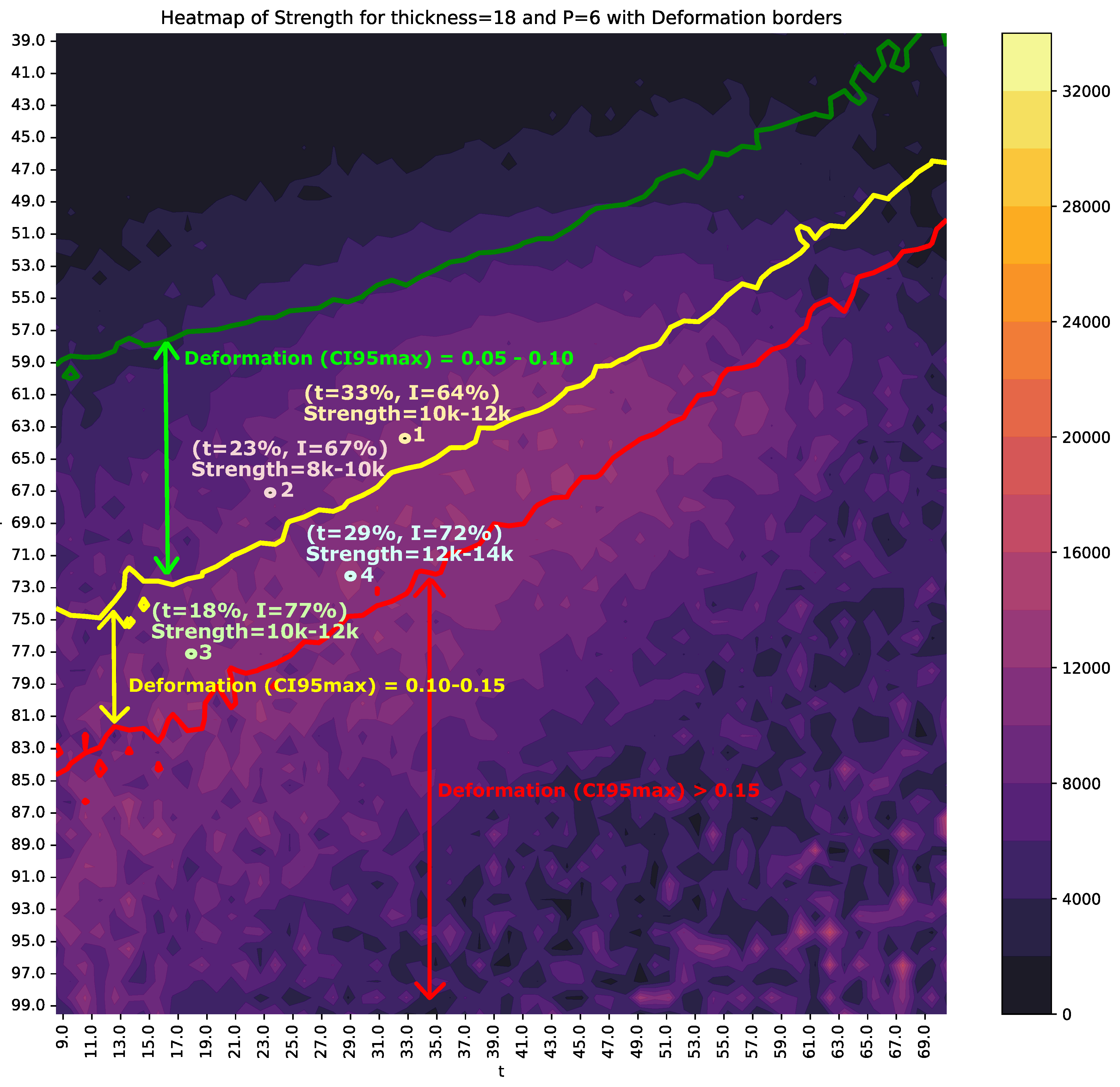
To support multi-criteria decision-making, the of S and of D are superimposed on these figures. The colored regions represent the values of S, while solid lines indicate the boundaries for D. Specifically, the green line corresponds to for D, the yellow line to , and the red line to .
Figure 10 shows the heat map for and . The area between the green and yellow lines represents a range of D between 0.05 and 0.10. If a maximum D of 0.10 is required, position 1 ( and ) would be appropriate, as it ensures a of S within 10000-12000N. However, this decision could be reconsidered if the objective is to further reduce time and energy consumption, albeit with a potential reduction in weld quality. For instance, position 2 represents an alternative operating point with shorter times, at the expense of reducing the S range to 8000-10000N.
Point 3 maintains the same S range as point 1 but halves the value of t, with a trade-off: higher energy consumption and reduced weld quality, as it falls within the range of D between 0.10 and 0.15. Lastly, point 4 increases the S range to 12000-14000N, although it lies within a smaller, isolated region of stability.
Another example is shown in Figure 11 for and . In this case, a viable option is position 1, with and , resulting in an S range between 20000 and 22000N. Alternatively, other operating points may be chosen to increase S: for instance, position 2 achieves a range of 22000-24000N with a reduction of t to 50% but an increase in I by 10%. Lastly, position 3 extends the time parameter, raising the S range to 24000-26000N, though with deformation values between 0.10 and 0.15.
7. Conclusions
The integration of Artificial Intelligence (AI) into industrial processes offers transformative potential, particularly in high-demand sectors like manufacturing, where process optimization is essential. However, a recurring challenge in this domain is the limited availability of data, which complicates the development of robust machine learning (ML) models. Small datasets increase the likelihood of overfitting, reducing the model’s ability to generalize to new scenarios, and can result in unstable performance under fluctuating production conditions.
This study introduces a novel ML-driven methodology specifically tailored to address these challenges within the context of resistance spot welding (RSW) for steel reinforcement bars. By leveraging a limited dataset, the proposed approach provides a framework for accurately predicting optimal welding parameters that balance critical objectives: weld quality, production efficiency, and energy consumption. Our methodology involves the systematic use of nested cross-validation and Bayesian optimization to ensure that the ML models are both highly accurate and robust. Additionally, the inclusion of AutoML techniques through the AutoGluon framework allowed for an efficient exploration of possible model configurations, further enhancing the robustness and reliability of the predictions.
The introduction of heat map-based decision support tools represents another significant contribution of this study. These visualizations enable production engineers to quickly identify stable operational zones within predefined criteria set by production managers, including quality thresholds, time constraints, and energy efficiency objectives. By using these dynamic heat maps, engineers are equipped to make real-time, data-driven decisions that optimize production parameters based on immediate needs, whether the priority is minimizing energy use, maximizing production speed, or ensuring high weld quality. This aligns with the growing industry focus on sustainable manufacturing practices, where energy efficiency and reduced resource consumption are increasingly prioritized.
The results of the study demonstrate that the selected ML models exhibit strong robustness across varying input conditions, maintaining stability even when the operational parameters fluctuate. This is particularly relevant given the energy-intensive nature of RSW processes and the increasing importance of minimizing energy costs in light of rising electricity prices. The confidence intervals included in the heat map visualizations add a layer of reliability, guiding production decisions that are not only optimal but also resilient to minor disturbances, thereby ensuring consistent weld quality and operational efficiency.
Future research can expand on this foundation by exploring more complex datasets or incorporating real-time sensor data to enable adaptive control systems. Additionally, integrating more sophisticated visualization tools or interactive user interfaces could enhance the practical usability of the decision support system, further supporting sustainable decision-making in industrial environments.
In conclusion, this work underscores the value of AI-driven decision support systems in industrial automation and establishes a scalable methodology for creating robust, reliable, and energy-conscious ML models, even when data is limited. This contribution is crucial for advancing sustainable manufacturing practices, offering a pathway for industries to optimize production processes without compromising on quality or efficiency.
Funding
This research received external funding from projects REGI2020/67, REGI2022/41 and REGI2020/41. It was also supported by grant PID2021-123219OB-I00 and PID2020-116641GB-I00 funded by Ministry of Science, Innovation and Universities of Spain and also by project INICIA 2023/02 funded by La Rioja Government (Spain).
Institutional Review Board Statement
Not applicable
Conflicts of Interest
The authors declare no conflicts of interest. The funders had no role in the design of the study; in the collection, analyses, or interpretation of data; in the writing of the manuscript; or in the decision to publish the results.
References
- Zhan, X.; Ou, W.; Wei, Y.; Jiang, J. The feasibility of intelligent welding procedure qualification system for Q345R SMAW. The International Journal of Advanced Manufacturing Technology 2015, 83, 765–777. [Google Scholar] [CrossRef]
- Gyasi, E.A.; Handroos, H.; Kah, P. Survey on artificial intelligence (AI) applied in welding: A future scenario of the influence of AI on technological, economic, educational and social changes. Procedia Manufacturing 2019, 38, 702–714. [Google Scholar] [CrossRef]
- Wang, X.; Zhang, Y.; Liu, J.; Luo, Z.; Zielinska, T.; Ge, W. Online detection of weld surface defects based on improved incremental learning approach. Expert Systems with Applications 2022, 195, 116407. [Google Scholar] [CrossRef]
- Satyro, W.C.; de Almeida, C.M.V.B.; Pinto Jr, M.J.A.; Contador, J.C.; Giannetti, B.F.; de Lima, A.F.; Fragomeni, M.A. Industry 4.0 implementation: The relevance of sustainability and the potential social impact in a developing country. Journal of Cleaner Production 2022, 337, 130456. [Google Scholar] [CrossRef]
- Matsushita, M.; Taniguchi, K.; Oi, K. Development of next generation resistance spot welding technologies contributing to auto body weight reduction. JFE Technical Report 2013, 18, 111–117. [Google Scholar]
- Goffin, N.; Jones, L.C.; Tyrer, J.; Ouyang, J.; Mativenga, P.; Woolley, E. Mathematical modelling for energy efficiency improvement in laser welding. Journal of Cleaner Production 2021, 322, 129012. [Google Scholar] [CrossRef]
- Ferreiro-Cabello, J.; Fraile-Garcia, E.; Lara-Santillán, P.M.; Mendoza-Villena, M. Assessment and Optimization of a Clean and Healthier Fusion Welding Procedure for Rebar in Building Structures. Applied Sciences 2020, 10, 7045. [Google Scholar] [CrossRef]
- Panda, B.N.; Babhubalendruni, M.V.A.R.; Biswal, B.B.; Rajput, D.S. Application of Artificial Intelligence Methods to Spot Welding of Commercial Aluminum Sheets (B.S. 1050). In Advances in Intelligent Systems and Computing; Springer India, 2014; pp. 21–32. [CrossRef]
- Zaharuddin, M.F.A.; Kim, D.; Rhee, S. An ANFIS based approach for predicting the weld strength of resistance spot welding in artificial intelligence development. Journal of Mechanical Science and Technology 2017, 31, 5467–5476. [Google Scholar] [CrossRef]
- Cho, Y.; Rhee, S. New technology for measuring dynamic resistance and estimating strength in resistance spot welding. Measurement Science and Technology 2000, 11, 1173–1178. [Google Scholar] [CrossRef]
- Wu, J.; Zhang, C.; Lian, K.; Cao, H.; Li, C. Carbon emission modeling and mechanical properties of laser, arc and laser–arc hybrid welded aluminum alloy joints. Journal of Cleaner Production 2022, 378, 134437. [Google Scholar] [CrossRef]
- Gujre, V.S.; Anand, R. Machine learning algorithms for failure prediction and yield improvement during electric resistance welded tube manufacturing. Journal of Experimental & Theoretical Artificial Intelligence 2019, 32, 601–622. [Google Scholar] [CrossRef]
- Jaypuria, S.; Bondada, V.; Gupta, S.K.; Pratihar, D.K.; Chakrabarti, D.; Jha, M. Prediction of electron beam weld quality from weld bead surface using clustering and support vector regression. Expert Systems with Applications 2023, 211, 118677. [Google Scholar] [CrossRef]
- Zhou, B.; Pychynski, T.; Reischl, M.; Kharlamov, E.; Mikut, R. Machine learning with domain knowledge for predictive quality monitoring in resistance spot welding. Journal of Intelligent Manufacturing 2022, 33, 1139–1163. [Google Scholar] [CrossRef]
- Panza, L.; Bruno, G.; Antal, G.; Maddis, M.D.; Spena, P.R. Machine learning tool for the prediction of electrode wear effect on the quality of resistance spot welds. International Journal on Interactive Design and Manufacturing (IJIDeM) 2024, 18, 4629–4646. [Google Scholar] [CrossRef]
- Zhang, Y.; Li, X.; Wang, Y.; Liu, Y.; Zhang, Y. A CNN-LSTM and Attention-Mechanism-Based Resistance Spot Welding Quality Online Detection Method for Automotive Bodies. Mathematics 2023, 11, 4570. [Google Scholar] [CrossRef]
- Chertov, A.; Maev, R.; Severin, F.; Gumenyuk, A.; Rethmeier, M. Real-Time AI driven Interpretation of Ultrasonic Data from Resistance Spot weld in Vehicle Structures Using Dynamic Resistance Adaptive Control. Materials Evaluation 2023, 81, 61–70. [Google Scholar] [CrossRef]
- Kraljevski, I.; Ju, Y.C.; Ivanov, D.; Tschöpe, C.; Wolff, M. How to Do Machine Learning with Small Data? – A Review from an Industrial Perspective. arXiv preprint arXiv:2311.07126, arXiv:2311.07126 2023.
- Pastor-López, I.; Sanz, B.; Tellaeche, A.; Psaila, G.; de la Puerta, J.G.; Bringas, P.G. Quality assessment methodology based on machine learning with small datasets: Industrial castings defects. Neurocomputing 2021, 456, 622–628. [Google Scholar] [CrossRef]
- Knauer, R.; Rodner, E. Squeezing Lemons with Hammers: An Evaluation of AutoML and Tabular Deep Learning for Data-Scarce Classification Applications. arXiv preprint arXiv:2405.07662, arXiv:2405.07662 2024.
- Merghadi, A.; Yunus, A.P.; Dou, J.; Whiteley, J.; ThaiPham, B. Machine learning methods for landslide susceptibility studies: A comparative overview of algorithm performance. Earth-Science Reviews 2020, 207, 103225. [Google Scholar] [CrossRef]
- Ware, C. Information visualization: perception for design; Morgan Kaufmann, 2019.
- Dimara, E.; Stasko, J. A Critical Reflection on Visualization Research: Where Do Decision Making Tasks Hide? IEEE Transactions on Visualization and Computer Graphics 2022, 28, 1128–1138. [Google Scholar] [CrossRef]
- Dimara, E.; Bailly, G.; Bezerianos, A.; Franconeri, S. Mitigating the Attraction Effect with Visualizations. IEEE Transactions on Visualization and Computer Graphics 2019, 25, 850–860. [Google Scholar] [CrossRef]
- Savikhin, A.; Maciejewski, R.; Ebert, D.S. Applied visual analytics for economic decision-making. 2008 IEEE Symposium on Visual Analytics Science and Technology, 2008, pp. 107–114. [CrossRef]
- Teo, C.H.; Nassif, H.; Hill, D.; Srinivasan, S.; Goodman, M.; Mohan, V.; Vishwanathan, S. Adaptive, Personalized Diversity for Visual Discovery. Proceedings of the 10th ACM Conference on Recommender Systems; Association for Computing Machinery: New York, NY, USA, 2016. [Google Scholar] [CrossRef]
- Antoniadi, A.M.; Du, Y.; Guendouz, Y.; Wei, L.; Mazo, C.; Becker, B.A.; Mooney, C. Current challenges and future opportunities for XAI in machine learning-based clinical decision support systems: a systematic review. Applied Sciences 2021, 11, 5088. [Google Scholar] [CrossRef]
- van Capelleveen, G.; van Wieren, J.; Amrit, C.; Yazan, D.M.; Zijm, H. Exploring recommendations for circular supply chain management through interactive visualisation. Decision Support Systems 2021, 140, 113431. [Google Scholar] [CrossRef]
- Zhai, Z.; Martínez, J.F.; Beltran, V.; Martínez, N.L. Decision support systems for agriculture 4.0: Survey and challenges. Computers and Electronics in Agriculture 2020, 170, 105256. [Google Scholar] [CrossRef]
- Watanabe, R.; Ishibashi, H.; Furukawa, T. Visual analytics of set data for knowledge discovery and member selection support. Decision Support Systems 2022, 152, 113635. [Google Scholar] [CrossRef]
- Ivanisevic, J.; Benton, H.P.; Rinehart, D.; Epstein, A.; Kurczy, M.E.; Boska, M.D.; Gendelman, H.E.; Siuzdak, G. An interactive cluster heat map to visualize and explore multidimensional metabolomic data. Metabolomics 2014, 11, 1029–1034. [Google Scholar] [CrossRef]
- AL-Barakani, A.; Bin, L.; Zhang, X.; Saeed, M.; Qahtan, A.S.A.; Hamood Ghallab, H.M. Spatial analysis of financial development’s effect on the ecological footprint of belt and road initiative countries: Mitigation options through renewable energy consumption and institutional quality. Journal of Cleaner Production 2022, 366, 132696. [Google Scholar] [CrossRef]
- Younesy, H.; Nielsen, C.; Möller, T.; Alder, O.; Cullum, R.; Lorincz, M.; Karimi, M.; Jones, S. An Interactive Analysis and Exploration Tool for Epigenomic Data. Computer Graphics Forum 2013, 32, 91–100. [Google Scholar] [CrossRef]
- Al-Kababji, A.; Alsalemi, A.; Himeur, Y.; Fernandez, R.; Bensaali, F.; Amira, A.; Fetais, N. Interactive visual study for residential energy consumption data. Journal of Cleaner Production 2022, 366, 132841. [Google Scholar] [CrossRef]
- Gu, Z.; Hübschmann, D. Make Interactive Complex Heatmaps in R. Bioinformatics 2021, 38, 1460–1462. [Google Scholar] [CrossRef]
- Gu, Z. Complex heatmap visualization. iMeta 2022, 1. [Google Scholar] [CrossRef]
- Wilke, C.O. Fundamentals of data visualization: a primer on making informative and compelling figures; O’Reilly Media, 2019.
- Yuan, J.; Chen, C.; Yang, W.; Liu, M.; Xia, J.; Liu, S. A survey of visual analytics techniques for machine learning. Computational Visual Media 2020, 7, 3–36. [Google Scholar] [CrossRef]
- Snoek, J.; Larochelle, H.; Adams, R.P. Practical bayesian optimization of machine learning algorithms. Advances in neural information processing systems 2012, 25. [Google Scholar]
- Vikhar, P.A. Evolutionary algorithms: A critical review and its future prospects. 2016 International Conference on Global Trends in Signal Processing, Information Computing and Communication (ICGTSPICC), 2016, pp. 261–265. [CrossRef]
- Shami, T.M.; El-Saleh, A.A.; Alswaitti, M.; Al-Tashi, Q.; Summakieh, M.A.; Mirjalili, S. Particle Swarm Optimization: A Comprehensive Survey. IEEE Access 2022, 10, 10031–10061. [Google Scholar] [CrossRef]
- Zhang, X.; Chan, F.T.; Yan, C.; Bose, I. Towards risk-aware artificial intelligence and machine learning systems: An overview. Decision Support Systems 2022, 159, 113800. [Google Scholar] [CrossRef]
- Vabalas, A.; Gowen, E.; Poliakoff, E.; Casson, A.J. Machine learning algorithm validation with a limited sample size. PLOS ONE 2019, 14, e0224365. [Google Scholar] [CrossRef]
- Morris, M.D. Factorial Sampling Plans for Preliminary Computational Experiments. Technometrics 1991, 33, 161–174. [Google Scholar] [CrossRef]
- Sobol’, I.M. Global sensitivity indices for nonlinear mathematical models and their Monte Carlo estimates. Mathematics and Computers in Simulation (MATCOM) 2001, 55, 271–280. [Google Scholar] [CrossRef]
Figure 1.
a) Fusion welding of reinforcement bars, b) Test bar configuration and weld strength failure (S).
Figure 1.
a) Fusion welding of reinforcement bars, b) Test bar configuration and weld strength failure (S).
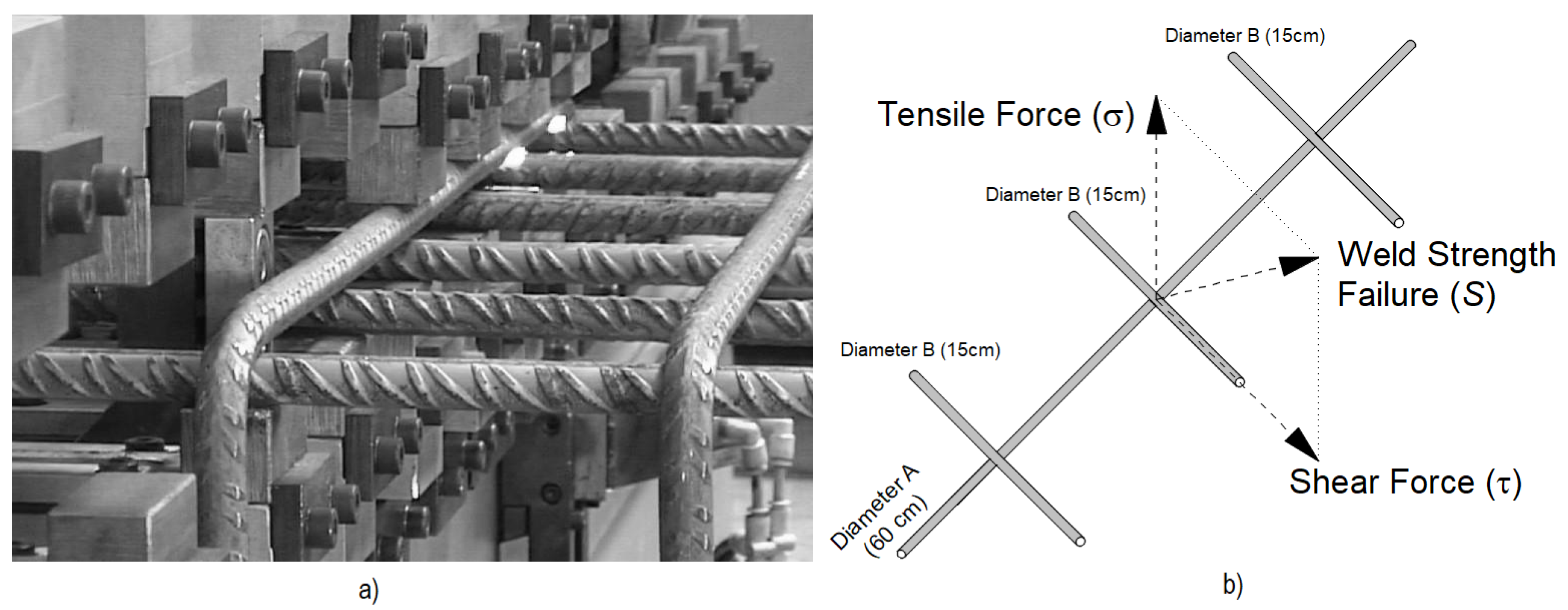
Figure 2.
Active welding time according to joint thickness, represented on a 0-100 scale.
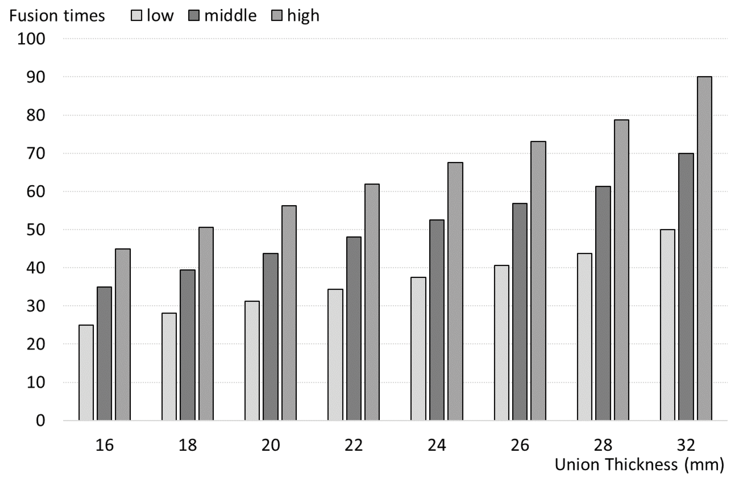
Figure 3.
Distribution of experiments according to the total joint thickness, .
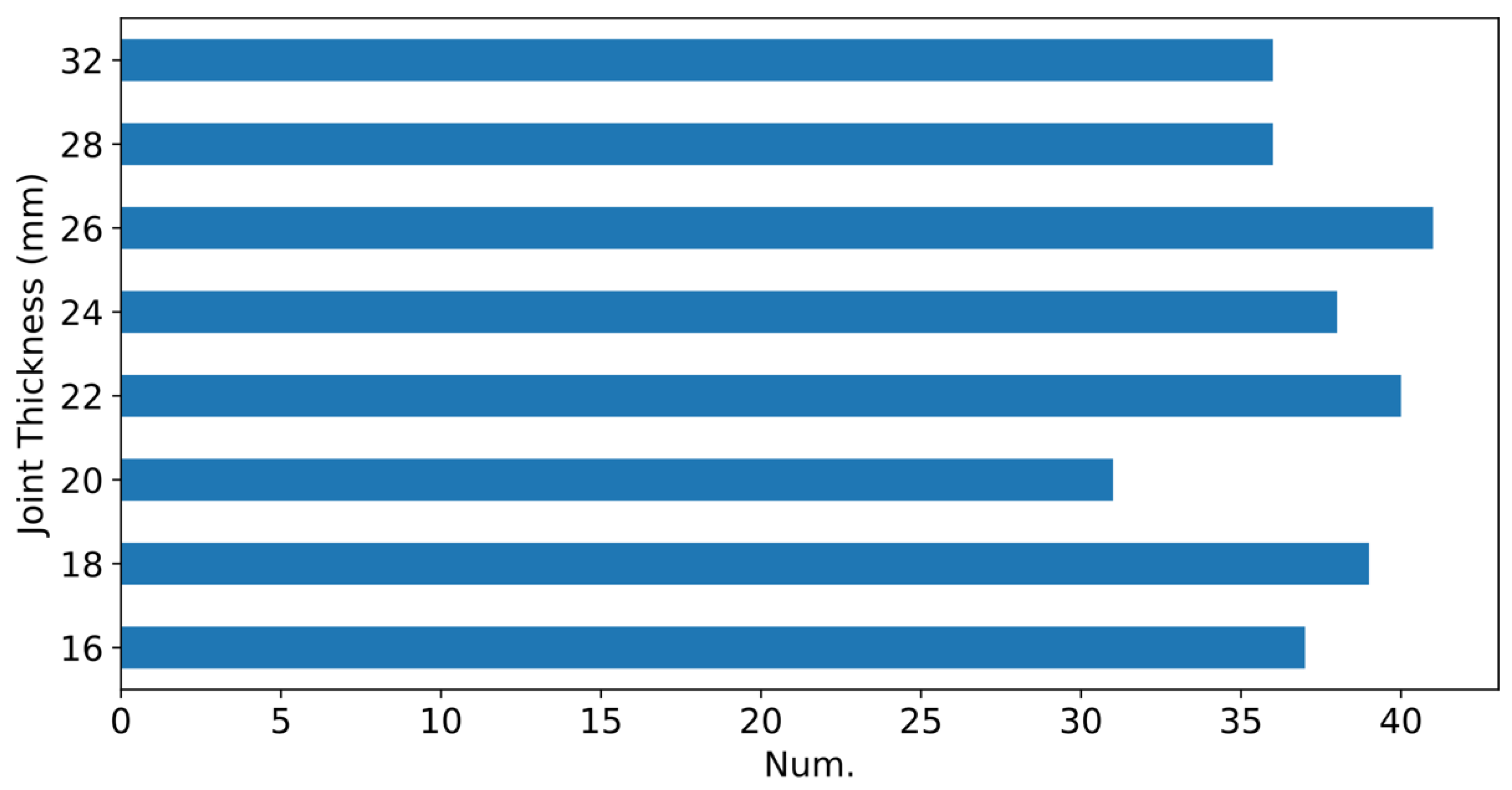
Figure 4.
Example of the inner loop within one iteration of the nested cross-validation process. The model is optimized using Bayesian optimization over 9 folds, while the test set remains untouched during this stage. The final model is evaluated on the test fold.
Figure 4.
Example of the inner loop within one iteration of the nested cross-validation process. The model is optimized using Bayesian optimization over 9 folds, while the test set remains untouched during this stage. The final model is evaluated on the test fold.
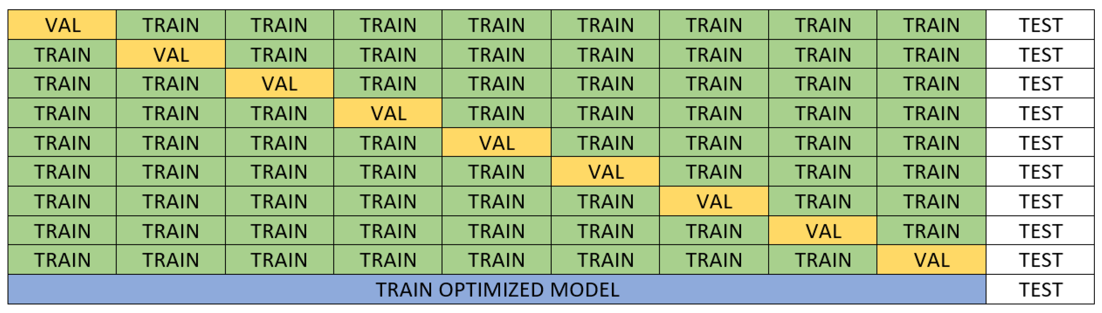
Figure 5.
Boxplots of the RMSE obtained with each algorithm for predicting weld strength.
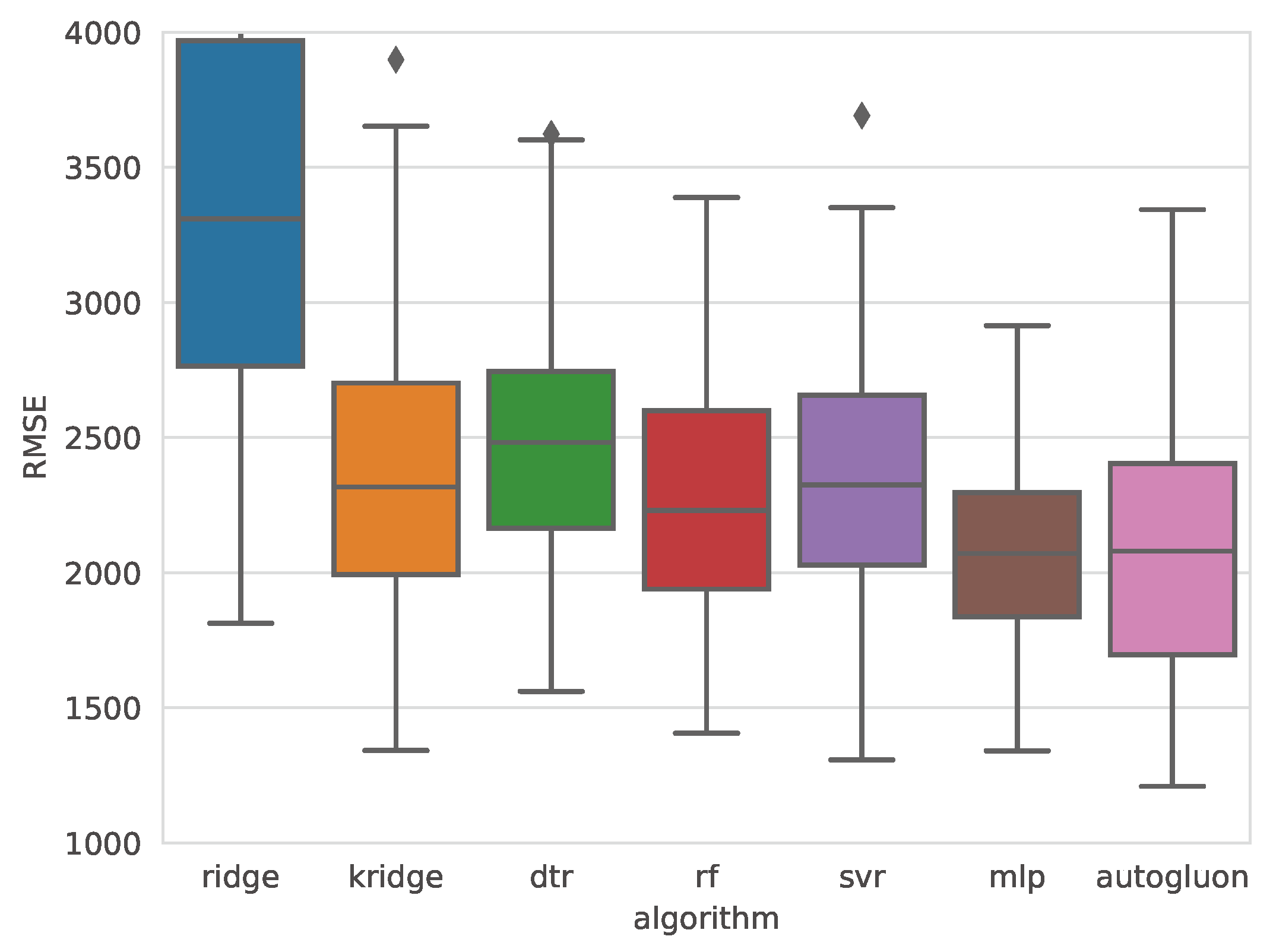
Figure 6.
Boxplots of the RMSE obtained with each algorithm for predicting weld deformation.
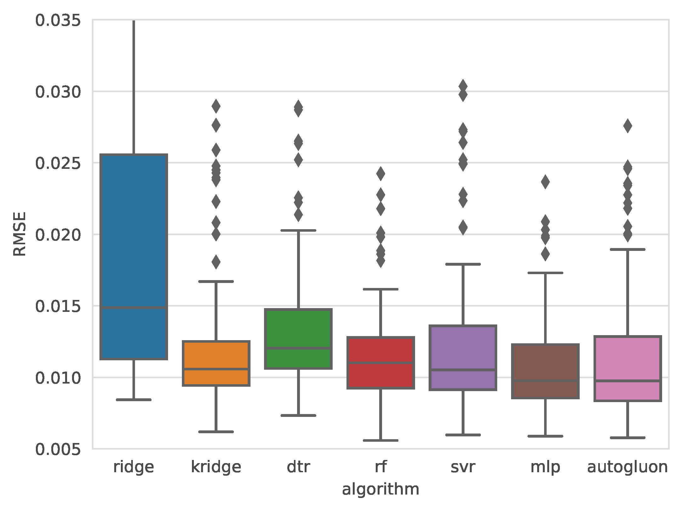
Figure 7.
Comparison of the RMSE distribution obtained with the MLP and Autogluon algorithms for weld strength.
Figure 7.
Comparison of the RMSE distribution obtained with the MLP and Autogluon algorithms for weld strength.
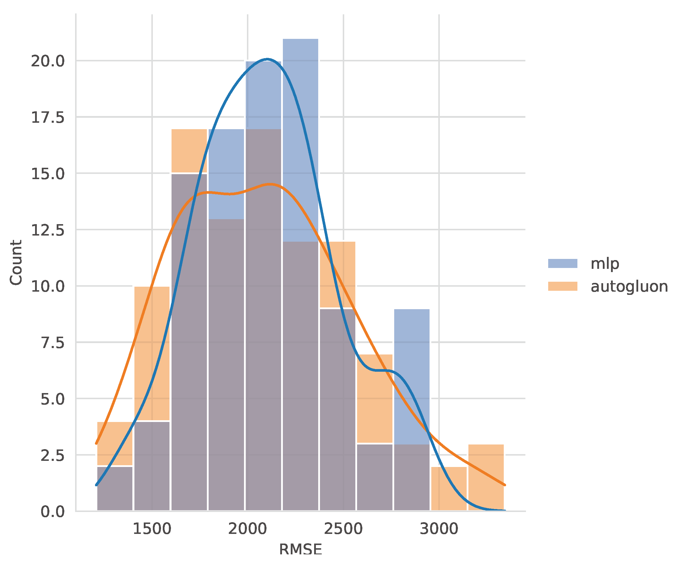
Figure 8.
Prediction of S with for each pair and six thickness values. The dashed lines indicate a 95% confidence interval and the continuous line is the average value. The red dashed line corresponds to the real value for each pair of values . The values of I and t correspond to the % of the maximum intensity and % of the maximum time in 2 seconds.
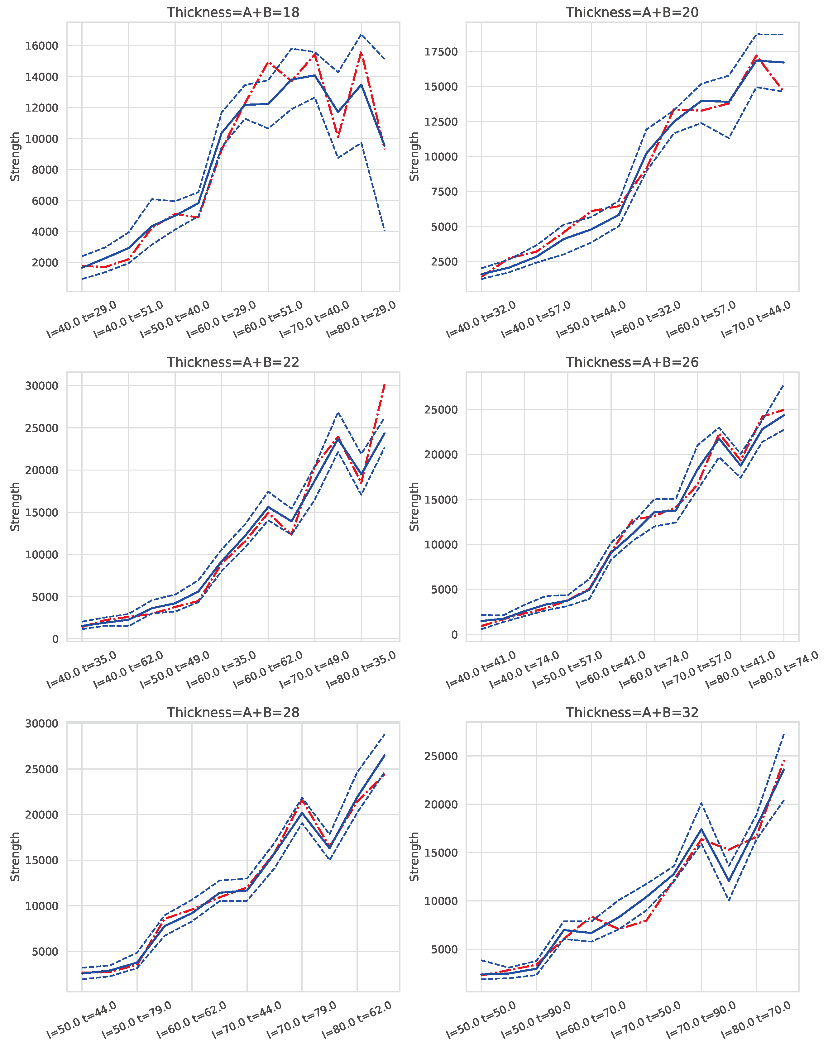
Figure 9.
Prediction of D with for each pair and six thickness values. The dashed lines indicate a 95% confidence interval and the continuous line is the average value. The red dashed line corresponds to the real value for each pair of values . The values of I and t correspond to the % of the maximum intensity and % of the maximum time in 2 seconds.
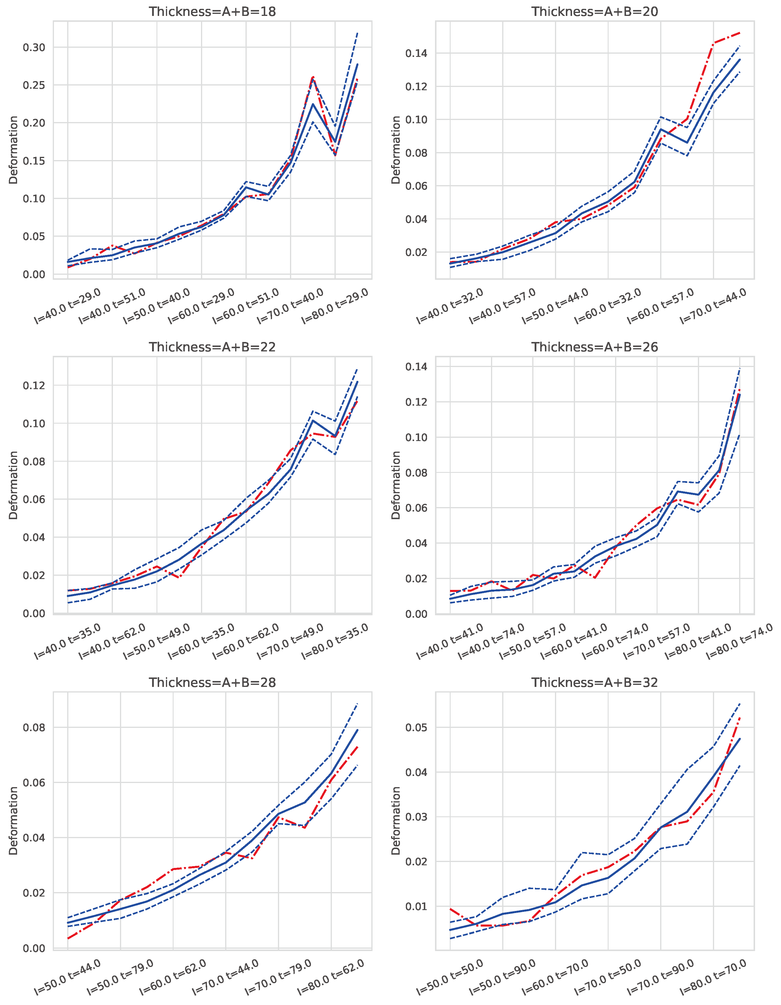
Figure 11.
Heat map displaying the value of S and of D for each combination of I and t, with and . The multi-colored vertical strip represents the value of S, while the green, yellow, and red contour lines denote values of D at levels of 0.05, 0.10, and 0.15, respectively. The values of I and t are expressed as percentages of the maximum intensity and maximum time (2 seconds) of the welding machine.
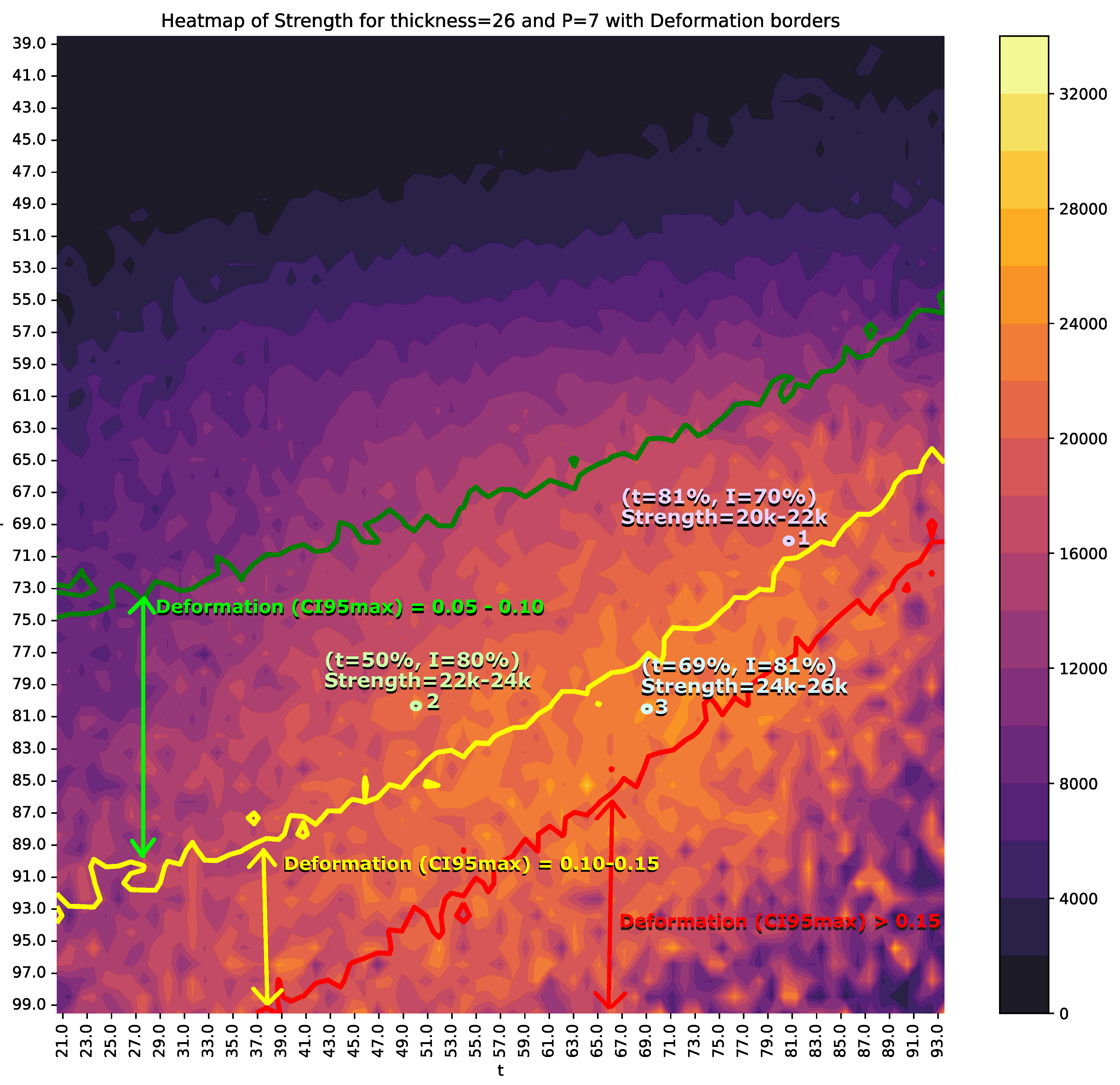

Table 1.
Combinations of diameters for joints Thickness
| Diameter A (mm) | Diameter B (mm) | Joint Thickness (mm) |
|---|---|---|
| 8 | 8 | 16 |
| 8 | 10 | 18 |
| 8 | 12 | 20 |
| 10 | 12 | 22 |
| 12 | 12 | 24 |
| 10 | 16 | 26 |
| 12 | 16 | 28 |
| 16 | 16 | 32 |
Table 2.
The welding parameter commands for the A-t-p equipment.
| Joint Thickness (mm) | Equipment Parameters | No. Specimen | |
|---|---|---|---|
| Phase-1 (Contact) | Phase-2 (Welding) | ||
| 16 | A*0.5 | 40%-50%-60%-70%-80% | 45 |
| t*1/3 | 25-35-45 | ||
| 5_6_7 | 5_6_7 | ||
| 18 | A*0.5 | 40%-50%-60%-70%-80% | 45 |
| t*1/3 | 29-40-51 | ||
| 5_6_7 | 5_6_7 | ||
| 20 | A*0.5 | 40%-50%-60%-70%-80% | 45 |
| t*1/3 | 32-44-57 | ||
| 5_6_7 | 5_6_7 | ||
| 22 | A*0.5 | 40%-50%-60%-70%-80% | 45 |
| t*1/3 | 35-49-62 | ||
| 5_6_7 | 5_6_7 | ||
| 24 | A*0.5 | 40%-50%-60%-70%-80% | 45 |
| t*1/3 | 38-53-68 | ||
| 5_6_7 | 5_6_7 | ||
| 26 | A*0.5 | 40%-50%-60%-70%-80% | 45 |
| t*1/3 | 41-57-74 | ||
| 5_6_7 | 5_6_7 | ||
| 28 | A*0.5 | 40%-50%-60%-70%-80% | 45 |
| t*1/3 | 44-62-79 | ||
| 5_6_7 | 5_6_7 | ||
| 32 | A*0.5 | 40%-50%-60%-70%-80% | 45 |
| t*1/3 | 50-70-90 | ||
| 5_6_7 | 5_6_7 | ||
Table 3.
ML models and ranges of the optimization of each hyperparameter.
| Algorithm | Tuning Hyperparameters |
|---|---|
| Ridge | |
| Kridge | |
| =rbf | |
| DTR | |
| RF | |
| SVR | |
| =rbf | |
| MLP | |
| =logistic |
Table 4.
Errors and best hyperparameters for S. Values are the average and the standard deviation (between parentheses) obtained with each algorithm and a 10-repeated 10-fold nested cross-validation (100 measures).
Table 4.
Errors and best hyperparameters for S. Values are the average and the standard deviation (between parentheses) obtained with each algorithm and a 10-repeated 10-fold nested cross-validation (100 measures).
| Algorithm | RMSE | MAE | MAPE | Hyperparameters |
|---|---|---|---|---|
| Autogluon | 2085.5(462.6) | 1486.9(291.2) | 16.2(3.2) | = |
| =5min | ||||
| MLP | 2104.3(363.7) | 1546.0(263.6) | 17.5(2.7) | =7.20(3.99) |
| =() | ||||
| =logistic | ||||
| RF | 2275.1(486.1) | 1623.6(320.1) | 17.3(3.4) | =17.97 (6.48) |
| =30.82(11.74) | ||||
| =() | ||||
| KRidge | 2350.2(497.0) | 1671.5(311.2) | 19.1(3.5) | =() |
| =() | ||||
| =rbf | ||||
| SVR | 2351.4(472.6) | 1644.9(299.0) | 18.8(3.4) | C=() |
| =() | ||||
| =rbf | ||||
| DTR | 2502.6(510.6) | 1840.3(356.3) | 19.7(3.9) | =14.72 (6.90) |
| =() | ||||
| Ridge | 3381.8(770.4) | 2366.8(440.1) | 25.6(4.9) | =() |
| = |
Table 5.
Errors and best hyperparameters for D. Values are the average and the standard deviation (between parentheses) obtained with each algorithm and a 10-repeated 10-fold nested cross-validation (100 measures).
Table 5.
Errors and best hyperparameters for D. Values are the average and the standard deviation (between parentheses) obtained with each algorithm and a 10-repeated 10-fold nested cross-validation (100 measures).
| Algorithm | RMSE | MAE | MAPE | Hyperparameters |
|---|---|---|---|---|
| MLP | 0.0109(0.0036) | 0.0077(0.0016) | 30.91(10.09) | =4.42(2.50) |
| =() | ||||
| =logistic | ||||
| Autogluon | 0.0114(0.0048) | 0.0077(0.0018) | 32.09(11.81) | = |
| =5min | ||||
| RF | 0.0117(0.0035) | 0.0083(0.0016) | 33.15(12.60) | =18.78 (6.35) |
| =32.43(10.94) | ||||
| =() | ||||
| KRidge | 0.0121(0.0049) | 0.0082(0.0018) | 32.25(11.49) | =() |
| =() | ||||
| =rbf | ||||
| SVR | 0.0125(0.0055) | 0.0083(0.0020) | 32.35(11.28) | C=() |
| =() | ||||
| =rbf | ||||
| DTR | 0.0133(0.0044) | 0.0097(0.0018) | 40.93(15.02) | =17.64 (7.18) |
| =() | ||||
| Ridge | 0.0198(0.0099) | 0.0114(0.0033) | 34.81(8.37) | =() |
| = |
Disclaimer/Publisher’s Note: The statements, opinions and data contained in all publications are solely those of the individual author(s) and contributor(s) and not of MDPI and/or the editor(s). MDPI and/or the editor(s) disclaim responsibility for any injury to people or property resulting from any ideas, methods, instructions or products referred to in the content. |
© 2024 by the authors. Licensee MDPI, Basel, Switzerland. This article is an open access article distributed under the terms and conditions of the Creative Commons Attribution (CC BY) license (http://creativecommons.org/licenses/by/4.0/).
Copyright: This open access article is published under a Creative Commons CC BY 4.0 license, which permit the free download, distribution, and reuse, provided that the author and preprint are cited in any reuse.


