Tool Wear Prediction Using Informer Architecture for Multi-Source Sensor Data Fusion

1.1. Research Background and Significance

In machining, tool wear exceeding its threshold affects workpiece quality. Real-time wear monitoring remains a key challenge. Ding [1] notes 22% of downtime is tool-related, constraining industry growth. This tech reduces downtime by 75%, boosts effective machining time to 60%, and increases machine utilization by 50% [2]. Demand for intelligent manufacturing underscores the value of real-time wear monitoring. The project aims for online wear monitoring and prediction, ensuring workpiece accuracy, machining continuity, and timely tool changes. This enhances cutting efficiency and automation, offering economic and social benefits, supporting advanced and intelligent manufacturing.

Figure 1.1. Tool wear at varying degrees.

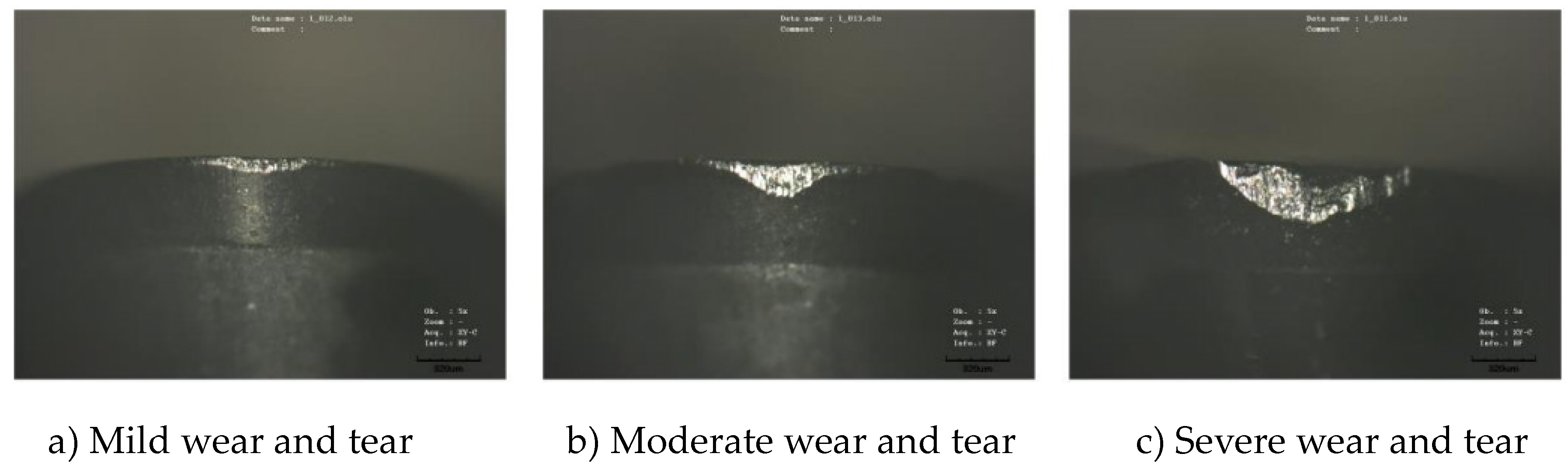
Figure 1.1. Tool wear at varying degrees.

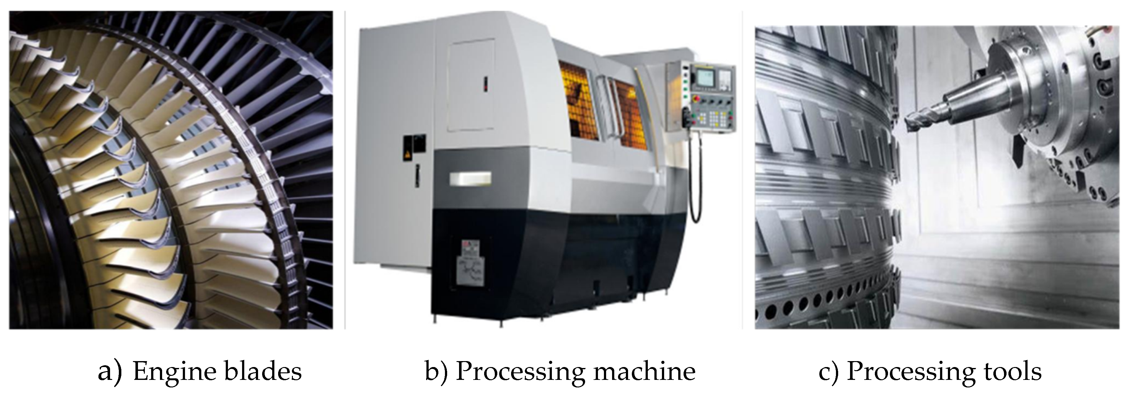
Engine blades, crucial components, are depicted in Figure 1.2 (a). They span aerospace, shipbuilding, and nuclear energy sectors. Blade performance impacts system efficiency, safety, and reliability. In national defense, economic development, and industrial systems, they are indispensable. Research [3] indicates blade failure is a common engine fault, threatening safety. Blade performance failure often leads to engine failure. Enhancing blade manufacturing accuracy is vital for improving engine efficiency, reducing failure rates, and boosting safety.

Engine blade manufacturing impacts final quality. Processes, shown in Figure 1.2, typically include CNC milling to create the flow channel (Figure 1.2 (b)). Cutting tools (Figure 1.2 (c)) are crucial in milling; wear impacts machining accuracy and workpiece quality, potentially disrupting the entire system and incurring significant losses.

Figure 1.2. Tool wear prediction technology diagram.

Figure 1.2. Tool wear prediction technology diagram.

In advanced tech era, industrial IoT and AI significantly impact engine blade processing. Intelligent CNC systems boost efficiency and quality. Tool wear, direct contact with workpiece [4], impacts quality and efficiency. Research shows 70-80% of tools replaced post-normal wear, 70% downtime from abnormal wear [5]. Abnormal wear causes waste and failures [6]. Predicting wear can reduce 75% abnormal downtime, boost efficiency 20-65% [7]. Tool replacement, essential for quality, traditionally relies on subjective judgment. Fixed automation methods often lead to waste or quality issues. Studying tool wear prediction is vital for ensuring quality, maximizing tool usage, cutting costs, and enhancing productivity.

1.2. Related Work

In traditional cutting, operators mainly use chip color, noise, or given chip time to identify tool wear manually. These subjective methods risk misjudgment. Alternatively, tools can be disassembled between processes for direct wear measurement, but this adds time and alignment issues, reducing accuracy. Traditional methods, reliant on human experience, are subjective, costly, and imprecise. With manufacturing intelligence, devices like computers, optical microscopes, sensors, and high-precision aids are integrated into processing. Researchers globally have made progress in tool wear monitoring and prediction. The following analyzes current research status (Figure 1.3).

Figure 1.3. Classification of Tool Wear Monitoring and Prediction Methods.

Figure 1.3. Classification of Tool Wear Monitoring and Prediction Methods.

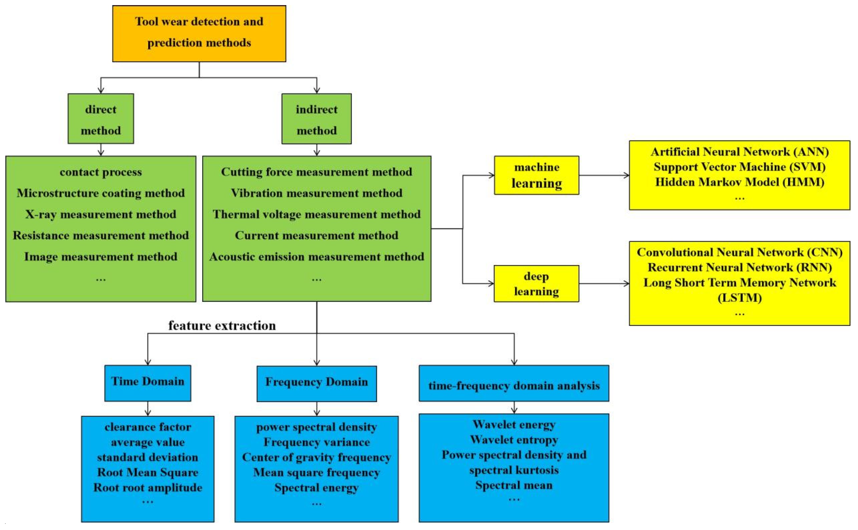
According to the form of monitoring, tool wear monitoring and prediction methods can be summarized and classified into two categories: direct methods and indirect methods [8].

(1) Direct method

The direct method measures tool wear directly via contact [9], computer vision [10,11], or radioactive tech [12,13]. These methods use auxiliary equipment to observe and measure wear changes, offering high accuracy but limited practical use, remaining experimental. For instance, while computer vision provides intuitive wear measurement through image processing, factors like machining environment, cutting fluid, and light can affect image quality, leading to inaccuracies. Radioactive elements also pose health risks to personnel.

(2) Indirect method

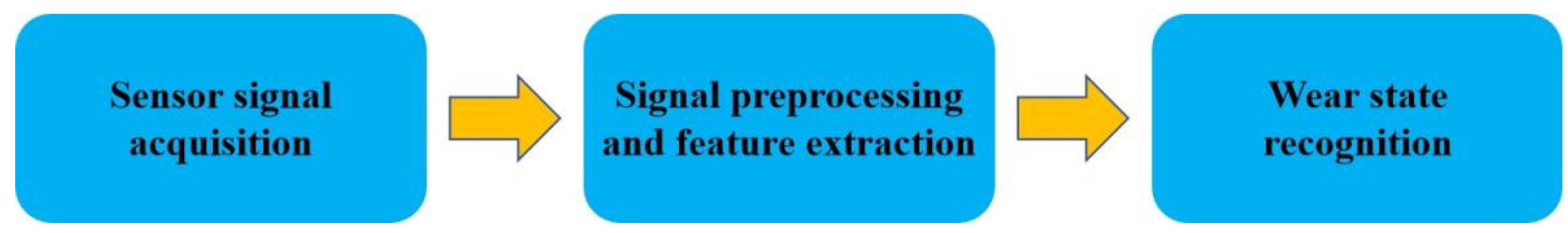
The indirect method monitors tool wear via cutting force [14], acceleration (vibration) [15], acoustic emission [16], and power [17], based on established mapping relationships. Cutting force is the most reliable signal. Liu [18] used monitored cutting force signals to achieve online wear monitoring. Zhao et al. [19] highlighted the significance of studying instantaneous contact stiffness’s effect on wear, crucial for controlling flank wear and enhancing cutter life. However, acceleration sensors are sensitive to vibrations and have strict installation requirements. Lin et al. [20] proved ensemble machine learning’s feasibility for wear monitoring. Acoustic emission, despite high-frequency advantages, is distance-sensitive, unsuitable for large workpieces. Current online monitoring leverages sensors and AI to form a comprehensive process from data acquisition to status recognition (Figure 1.4), summarizing key steps into three main parts.

(1) Selection and Collection of Monitoring Signals

It is mainly based on different processing types, processing methods, and processing requirements to select appropriate sensors to collect the corresponding required signals. For example, acceleration sensors require high installation positions, and acoustic emission sensors are not suitable for large workpieces.

(2) Signal preprocessing and feature extraction

After a series of preprocessing measures, the collected monitoring signals are processed to obtain ideal signal data. Then, feature information related to changes in wear degree or wear value is extracted and constructed into feature vectors as inputs for subsequent models.

(3) Wear state recognition

Specifically, wear state recognition should be based on obtaining wear values to determine the degree of wear. This process is achieved by exploring the mapping relationship between the feature vectors of the extracted signals and the wear values, constructing corresponding mathematical models, and monitoring the wear values and tool status.

Figure 1.4. Tool wear condition monitoring framework.

Figure 1.4. Tool wear condition monitoring framework.

1.2.1. Research Status of Feature Extraction Methods for Monitoring Signals

For signal information related to cutting force, vibration, and current indirectly measured by sensors and tool wear, effective values are generally extracted as feature quantities using time-domain analysis [21], frequency-domain analysis [22], and time-frequency domain analysis. These feature quantities are then combined into feature vectors for monitoring or prediction. The summary of feature extraction methods for sensor monitoring signals is shown in Table 1.1.

Table 1.1. Summary of common feature extraction methods.

Analysis method	Common method	Evaluate
Time Domain	Mean, variance, skewness, kurtosis, etc	Simple calculation, easily affected by unstable factors during cutting process
Frequency Domain	Amplitude, phase, power, intensity, etc	Widely used for tool wear
Time-frequency domain analysis	Wigner analysis, wavelet analysis, etc	Suitable for processing non-stationary signals, adaptive

Table 1.1. Summary of common feature extraction methods.

Analysis method	Common method	Evaluate
Time Domain	Mean, variance, skewness, kurtosis, etc	Simple calculation, easily affected by unstable factors during cutting process
Frequency Domain	Amplitude, phase, power, intensity, etc	Widely used for tool wear
Time-frequency domain analysis	Wigner analysis, wavelet analysis, etc	Suitable for processing non-stationary signals, adaptive

The collected monitoring signals are typically in the time domain, with time-domain analysis using probability and statistical methods to calculate signal characteristics via simple formulas. Conversely, tool wear can cause changes in signal frequency, necessitating frequency-domain analysis. Time-frequency analysis, combining time and frequency domains, is mainly used for time-varying non-stationary signals, making it the most common and important method in wear signal feature processing. Techniques like Wigner time-frequency analysis, wavelet analysis, and Hilbert Huang transform have been proposed, with wavelet analysis widely used as an efficient tool.

Li [23] utilized DB8 as the wavelet basis for 4-layer wavelet packet decomposition on current signals, using mean and variance of each frequency component as features for wear state monitoring. Harun [24] applied time-frequency analysis to three-axis vibration signals in deep hole drilling to detect tool malfunctions. Kumar [25] used wavelet analysis for bearing vibration signals to detect fault categories, optimizing mother wavelet selection. Yoon [26] demonstrated that wavelet transform is more suitable for non-stationary tool wear monitoring signals than FFT.

1.2.2. Research Status of Tool Wear Monitoring and Prediction Methods

Pattern recognition methods are constantly innovating with the rapid development of artificial intelligence. Based on the aforementioned feature extraction techniques, researchers establish a mapping relationship between sensor monitoring signals and tool wear through machine learning, deep learning, and other methods to monitor or predict tool wear.

(1) Machine learning

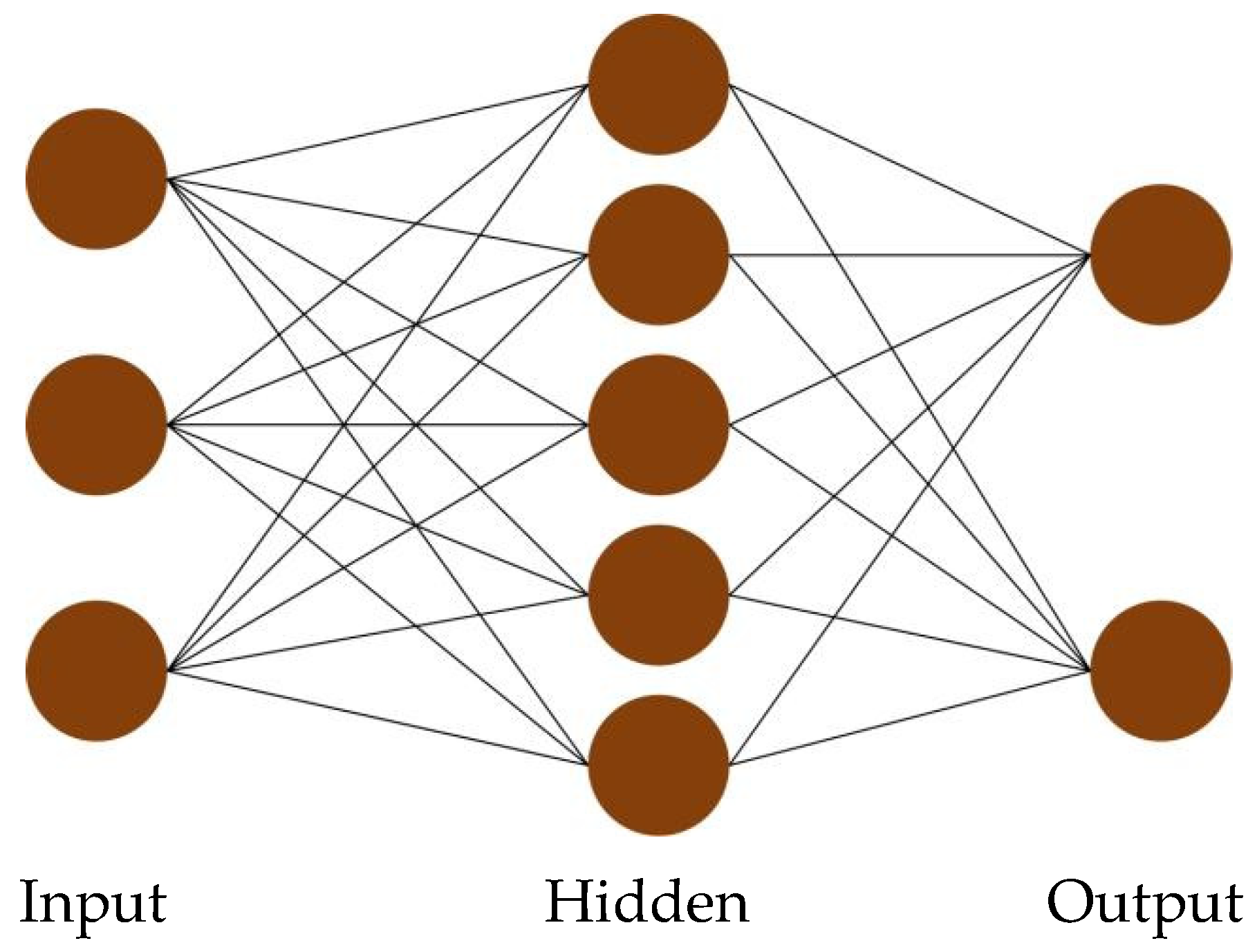
Common machine learning methods in tool wear monitoring include Artificial Neural Network (ANN), Support Vector Machine (SVM), and Hidden Markov Model (HMM). As seen in Figure 1.5, ANN processes features of sensor signals through an input layer, a hidden layer involving various neuron connections, and an output layer to predict tool wear. Drouillt [27] used ANN for tool life prediction, Wiciak [28] for milling tool wear based on force and vibration signals, and Feito [29] for analyzing thrust impact during composite material drilling with an ANN-based control system, guiding industrial applications.

Figure 1.5. Schematic Diagram of Artificial Neural Network.

Figure 1.5. Schematic Diagram of Artificial Neural Network.

SVM, renowned for its superior learning and decision-making abilities, is widely utilized in tool wear monitoring. Cheng [30] enhanced tool wear state classification accuracy by integrating SVM with particle filtering. Albina [31] developed a particle board drilling tool wear classification model using SVM with parameters like cutting feed, torque, vibration, and acoustic emission. Pandiyan [32] refined time-frequency domain features via genetic algorithms for SVM-based grinding tool wear classification. SVM, less prone to human intervention and effective for small sample problems, outperforms ANN in deterministic structures. HMM, as a statistical analysis-based recognition model, has been applied in fault diagnosis. LV [33] processed milling force signal features through a self-organizing mapping neural network, encoding them for discrete HMM training to determine wear states based on stage probabilities.

(2) Deep learning

The aforementioned feature extraction methods, involving manual selection and feature vector construction, can be subjective and may not fully capture tool wear conditions. With advances in computing power, data-driven deep learning has emerged as a key AI research area. In tool wear monitoring, sensor data accumulation has spurred the adoption of data-intensive deep learning methods. Researchers increasingly utilize deep neural networks for adaptive feature extraction, demonstrating deep learning’s superiority over traditional machine learning methods [34]. For instance, Kothuru et al [35] applied convolutional neural networks (CNNs) to create a deep model for tool state monitoring, analyzing machining sound signals’ spectral characteristics to achieve successful tool wear monitoring.

WU et al. [36] presented a hybrid deep learning model for predicting tool wear states in ultra-precision diamond cutting, estimating cutting forces and forecasting diamond tool wear using signals like motion displacement and velocity. Cao et al. developed a CNN based on the translation-invariant wavelet framework, validating its feasibility and efficacy in recognizing milling tool wear through experiments on steel workpieces with varying parameters. Tang et al. [37] trained a 12-layer deep residual network using the PHM dataset, eliminating the need for feature extraction and improving performance over traditional methods.Zhimeng Li et al. [38] introduced a clustering-based TCM system adaptable to different machining conditions, including variable cutting parameters, tools, and methods.Li et al. [39] proposed a CNN-based data-driven approach for predicting RUL, but as data complexity grows, the model’s handling capacity becomes limited, leading to reduced prediction accuracy.

Given the nonlinear characteristics of tool wear curves, LSTM neural networks effectively manage time series data. Wu [40] leverages LSTM’s memory capabilities for industrial applications, achieving robust RUL prediction by capturing long-term dependencies in monitoring signal series. Hinchi [41] proposed an end-to-end RUL framework, using convolutional layers for feature extraction from monitored signals, followed by LSTM for wear process information, and fully connected layers for lifespan prediction. He [42] established an LSTM-CNN network to extract multi-dimensional features from signal data, validating its monitoring performance with the PHM dataset. GRU, with its simpler structure, also handles time series data. Yan [43] combined CNN and GRU to propose a wear value prediction method using a CNN-BiGRU network, enhancing accuracy through edge data processing. Wang [44] used GRU to build a deep heterogeneous model considering sequence information dependency, inputting multiple past tool wear data to predict the next wear value, achieving single-step prediction but not consecutive wear value prediction. Previous studies were conducted under specific conditions, neglecting varying machining parameters like cutting and tool materials. In complex actual machining processes, model applicability weakens, leading to inaccurate monitoring and prediction. Li [45] extracted multiple effective features from current and vibration signals, clustering the features under different operating conditions using K-means to enhance model applicability while maintaining accuracy. Wan Peng et al [46] introduced a wear prediction method based on a domain adversarial gate control network, considering complex working condition information like tool parameters and materials, achieving accurate wear value prediction with a small amount of labeled sample data.

1.3. Current Shortcomings

Improved RNN networks, such as LSTM and GRU, address the long-term dependency problem in time series, but existing research assumes uniform weight for all time points, implying equal impact of past inputs on future predictions. However, in practical scenarios, the influence of historical inputs on future predictions varies over time. For instance, tool wear information closer to the prediction point has a greater impact than that farther away. This suggests that the impact of past tool wear status on future predictions is not uniform.

In machine tool processing, the states at points B and C are more similar, so B’s impact on C should be greater than A’s. This concept aligns with the Attention mechanism in NLP, which assigns varying weights to sequence inputs to focus on more critical information. This has proven effective in tasks like machine translation and image recognition.

Figure 1.6. Schematic Diagram of Tool Wear Curve.

Figure 1.6. Schematic Diagram of Tool Wear Curve.

Existing studies focus on single working conditions. In actual cutting processes, conditions often vary. Research on wear monitoring under multiple conditions is limited, requiring comprehensive analysis from diverse angles for accurate monitoring and prediction, offering practical guidance for multi-condition processing.

Ensuring machining accuracy and process stability necessitates timely tool replacement when wear reaches a critical level. Advance wear prediction ensures optimal tool change timing.

1.4. Contribution

Research on tool wear is crucial for the intelligent advancement of machining and manufacturing. Despite existing studies, challenges persist, especially in forecasting future wear and understanding wear under diverse conditions. To tackle these, this paper proposes a multi-step tool wear prediction algorithm using Informer, addressing sensor data preprocessing, wear status monitoring, and wear value prediction.

Chapter 1: Introduction

This chapter outlines the significance of tool wear research, reviewing current studies on sensor signals, feature extraction, and status monitoring. It identifies gaps and defines the research scope.

Chapter 2: Signal Analysis and Preprocessing

A theoretical overview of tool wear, including principles, forms, and processes, is provided. The experimental dataset is introduced, with analyses of sensor signals and wear values. Invalid and abnormal data are identified and processed, ensuring data integrity.

Chapter 3: Core Framework and Model Construction

This chapter develops a multi-step prediction framework for tool wear, including a state monitoring model and a wear prediction model. The state monitoring model ensures real-time wear status analysis, aiding timely detection and tool management. The wear prediction model, leveraging an encoding-decoding structure and the Informer model with an Attention mechanism, achieves accurate multi-step wear value predictions, enhancing tool management efficiency and cost reduction.

Chapter 4: Conclusions

Experimental comparisons validate the Informer model’s effectiveness in capturing complex long short-term dependencies, significantly improving wear prediction accuracy. The conclusion summarizes the work and outlines future research directions.

2.1. Overview of Tool Wear

During cutting, complex physical interactions among the tool, workpiece surface, and chips occur, involving forces like friction, shear, and compression. These interactions create local high temperatures on the tool’s contact surface, affecting tool performance and altering chip states. Elevated temperatures soften chip materials, causing adhesion that degrades tool surface quality. Continuous processing roughens the tool’s surface due to attachments, increasing friction. Increased friction reduces contact efficiency, leading to heat accumulation and severe wear. Repeated high temperatures and wear progressively destroy the tool’s oxidation protective layer, diminishing its protective function.

The destruction of the oxidation protective layer and intensification of tool wear are complementary processes. As wear increases, it decreases tool surface performance and affects overall cutting process efficiency. This results in higher cutting forces and temperatures, reducing machining accuracy and surface quality. Tool wear can also cause issues like chipping and unstable cutting, negatively impacting machining quality and efficiency. As wear intensifies, system vibrations, increased cutting forces, and elevated temperatures occur, potentially damaging workpieces and machine tools [47,48]. To better study tool wear prediction, this section outlines the forms and processes of tool wear.

2.1.1. Form of Tool Wear

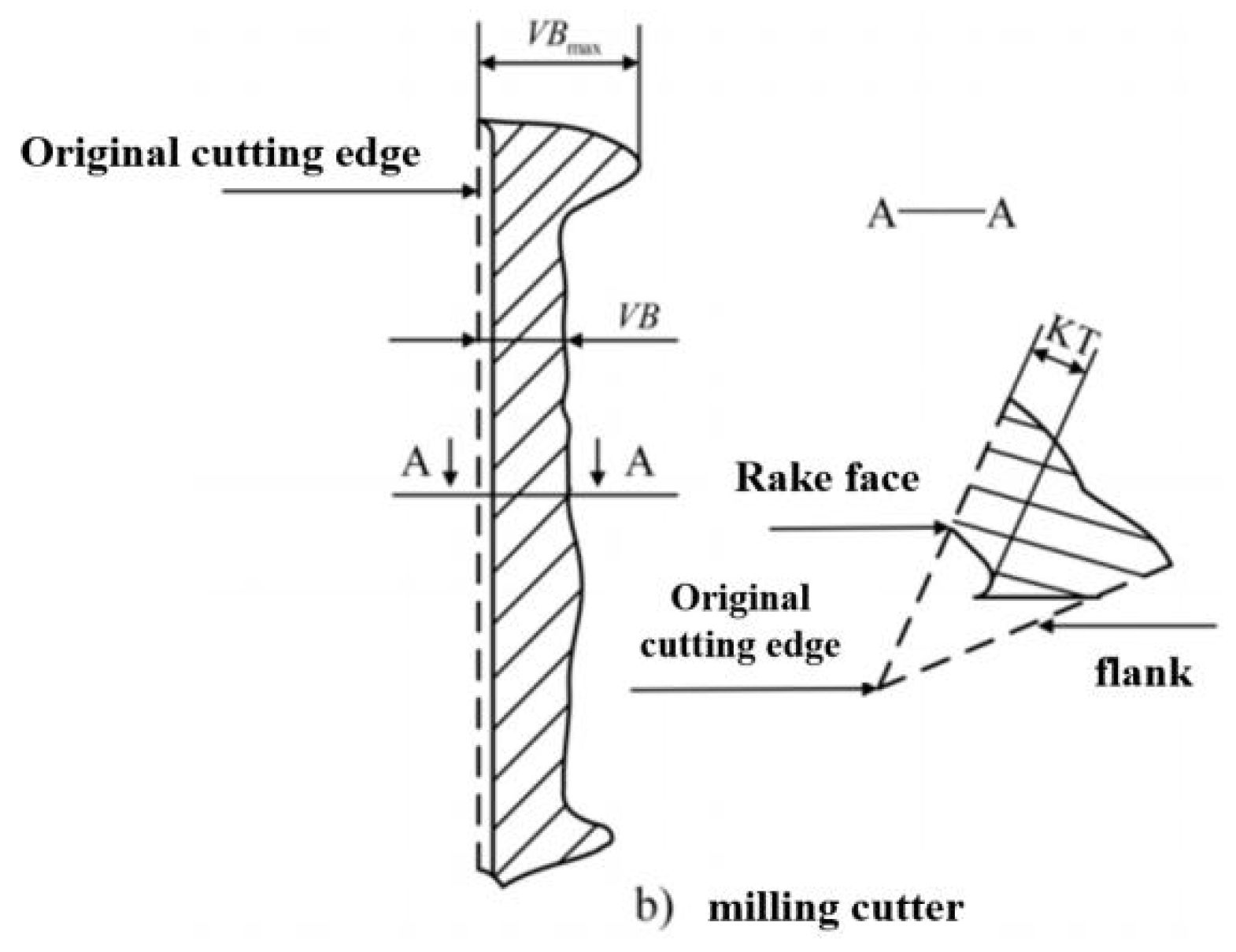
According to tool wear mechanisms, contact friction at various tool positions leads to different wear forms, categorized into normal and abnormal wear [49,50,51]. This article focuses on normal wear, where wear value gradually increases with machining time. Practical tool wear can be detailed by location and form (Table 2.1), aiding systematic analysis under varying cutting conditions. Figure 2.1 visually aids in identifying wear areas: the front cutting surface shows crescent-shaped grooves (quantified by KT), formed by cutting-induced high temperatures and stress altering the tool’s microstructure. The rear blade shows linear, uneven edge wear (represented by VB), influenced by the large contact area with the workpiece and its ease of observation, making VB crucial for wear assessment.

In actual machining, rear cutting surface wear significantly impacts workpiece accuracy. Hence, tool managers commonly use back face wear value VB as the primary wear indicator. This choice enhances measurement and monitoring efficiency, accurately predicts remaining tool life, enabling timely maintenance or replacement. This ensures cutting process stability and product quality.

Table 2.1. Classification of Normal Wear Forms of Cutting Tools.

Wear Pattern	Describe
crater wear	Wear caused by friction between chips and the front cutting surface
Flank wear	Wear caused by compression and friction between the workpiece surface and the back cutting surface
Boundary wear	The grooves generated by the contact between the main and auxiliary cutting edges and the surface of the workpiece

Table 2.1. Classification of Normal Wear Forms of Cutting Tools.

Wear Pattern	Describe
crater wear	Wear caused by friction between chips and the front cutting surface
Flank wear	Wear caused by compression and friction between the workpiece surface and the back cutting surface
Boundary wear	The grooves generated by the contact between the main and auxiliary cutting edges and the surface of the workpiece

Figure 2.1. Normal forms of tool wear.

Figure 2.1. Normal forms of tool wear.

2.1.2. Tool Wear Process

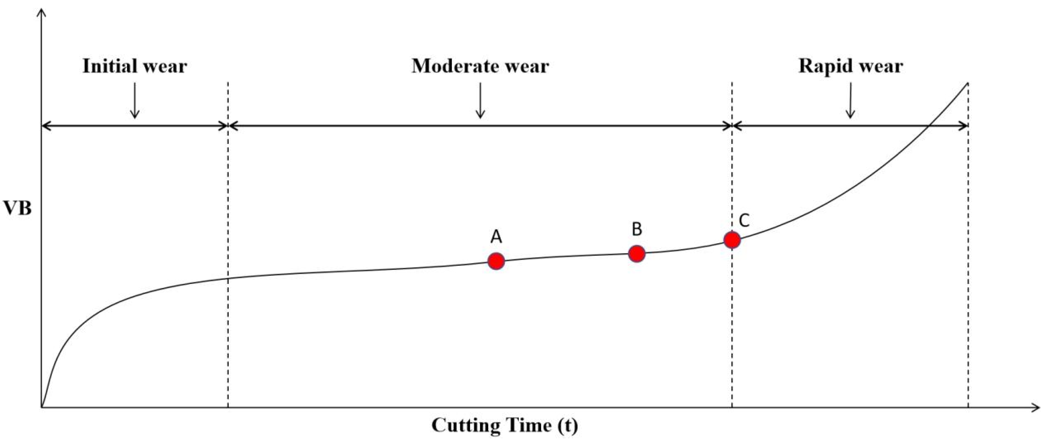
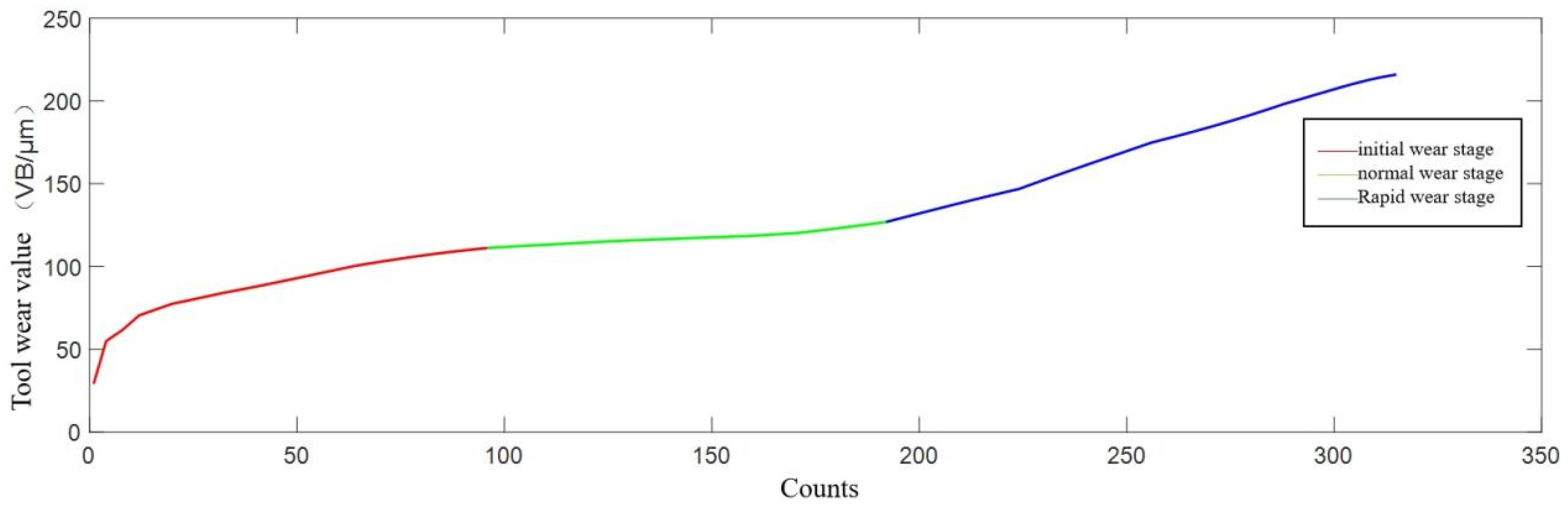
Tool wear is a non-linear, positively correlated process with cutting time, influenced by tool material, workpiece properties, and machining parameters. Despite minor variations, wear processes show high similarity under consistent conditions. The wear curve (Figure 2.2) illustrates tool wear’s gradual increase, with significant growth at specific time points.

Figure 2.2. Tool Wear Curve.

Figure 2.2. Tool Wear Curve.

Figure 2.2’s axes denote cutting time t and wear value VB. Alternatively, fixed cutting strokes and tool runs measure wear value. A tool’s life cycle has three main stages: initial wear, normal wear, and rapid wear [52,53].

Initial wear stage: New tool’s thin, sharp edge in line contact with workpiece surface. Small back face contact area causes significant stress, coupled with unfamiliarity with material properties, leading to faster initial wear of the back cutting surface, consuming less cutting time.

Moderate wear stage: After initial wear, tool adapts to workpiece material. Back cutting surface smoothens, rounding, reducing stress with increased contact area. Wear rate significantly drops, stabilizing, with minimal fluctuations. This phase, representing the stable machining period, dominates tool life cycle, ensuring stable and reliable part quality.

Rapid wear stage: After prolonged normal wear, tool wear exceeds a threshold, entering rapid wear. Reduced tool hardness causes sharp increases in cutting force and temperature, rapidly accelerating wear. Workpiece surface quality degrades. Excessive wear renders tool ineffective, risking damage to workpiece and machine tool. Rapid wear phase is brief; monitoring tool status and timely replacement are crucial to minimize losses.

2.2. Tool Wear Dataset

This section mainly introduces the dataset and experimental setup used in the experiment, and visualizes and analyzes the sensor signals and corresponding wear values in the dataset.

2.2.1. Introduction to the Single Condition Tool Wear Dataset

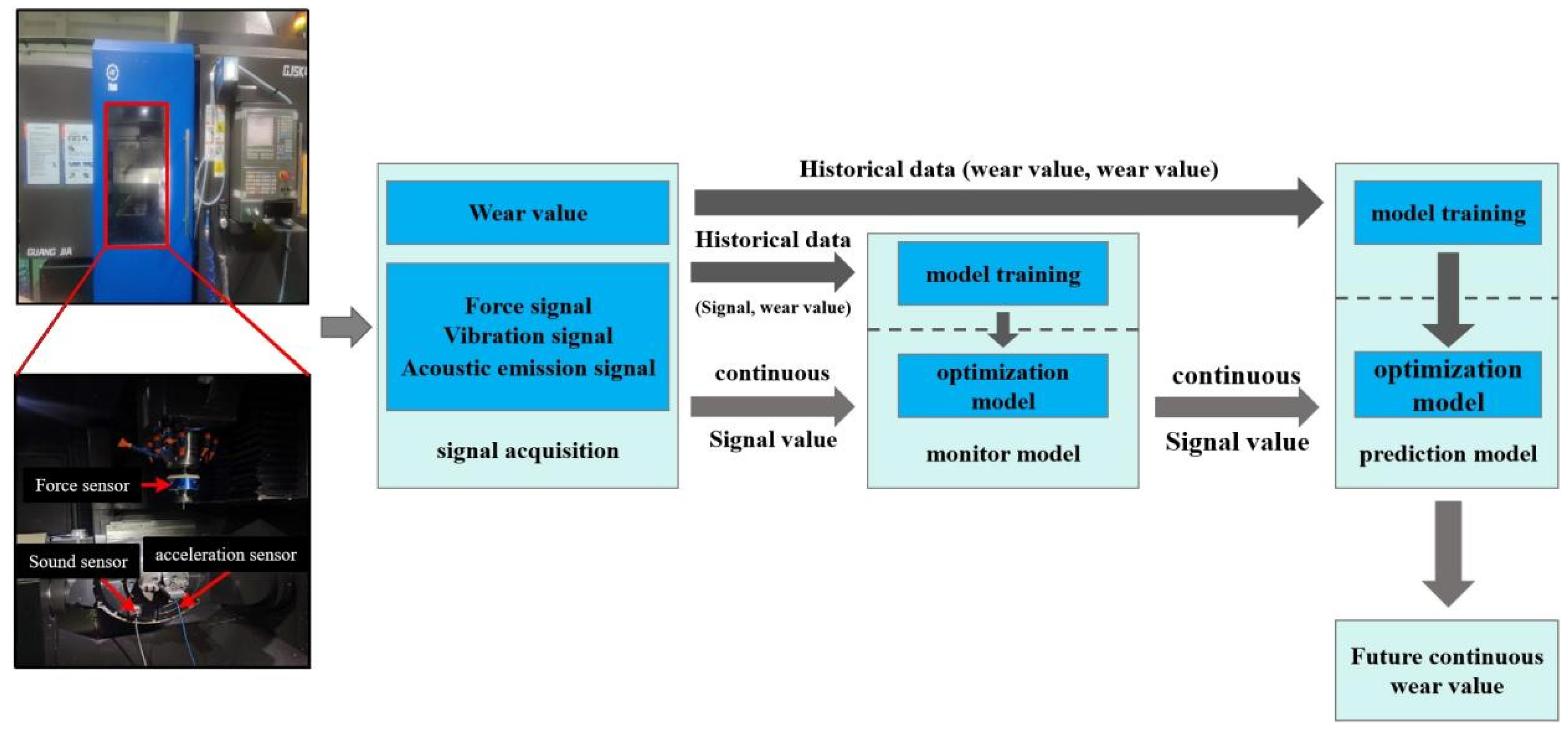
Single condition experimental data in this article is sourced from the PHM 2010 milling dataset, available from the 2010 AAPHM High Speed CNC Machine Health Prediction Competition. Milling process is depicted in Figure 2.3. The experimental setup in Figure 2.4 includes main equipment and processing parameters listed in Table 2.2 and 2.3. Experiment employed sensors for cutting force, vibration, and acoustic emission signals. Figure 2.2 shows three accelerometers at workpiece’s three axial positions to collect vibration signals. Acoustic emission sensor is mounted directly on the workpiece, and a triaxial force gauge between worktable and workpiece captures three-axis cutting force signals. Specific signals collected are detailed in Table 2.4.

Figure 2.3. Experimental diagram of milling with tool wear.

Figure 2.3. Experimental diagram of milling with tool wear.

Figure 2.4. Schematic diagram of experimental platform.

Figure 2.4. Schematic diagram of experimental platform.

This section mainly introduces the dataset and experimental setup used in the experiment, and visualizes and analyzes the sensor signals and corresponding wear values in the dataset.

Table 2.2. Main Experimental Equipment.

Hardware Conditions	Model and Main Parameters
CNC milling machine	High speed CNC machine tool Roders Tech RFM760
Dynamometer	Kistler 9265B triaxial force gauge
Charge Amplifier	Kistler5019A
Workpiece material	Inconel 718
Cutting tool	Ball end hard alloy milling cutter
Data acquisition card	NI DAQ PCI 1200
Wear measuring device	LEICA MZ12 microscope

Table 2.2. Main Experimental Equipment.

Hardware Conditions	Model and Main Parameters
CNC milling machine	High speed CNC machine tool Roders Tech RFM760
Dynamometer	Kistler 9265B triaxial force gauge
Charge Amplifier	Kistler5019A
Workpiece material	Inconel 718
Cutting tool	Ball end hard alloy milling cutter
Data acquisition card	NI DAQ PCI 1200
Wear measuring device	LEICA MZ12 microscope

Table 2.3. Experimental Processing Parameters.

Cutting Conditions	Spindle Speed	Feed Speed	Axial Cutting Depth	Radial Cutting Depth	Feed Rate	Sampling Frequency
parameter	(r/min)	(mm/min)	(mm)	(mm)	(mm)	(kHz)
	10400	1555	0.2	0.125	0.001	50

Table 2.3. Experimental Processing Parameters.

Cutting Conditions	Spindle Speed	Feed Speed	Axial Cutting Depth	Radial Cutting Depth	Feed Rate	Sampling Frequency
parameter	(r/min)	(mm/min)	(mm)	(mm)	(mm)	(kHz)
	10400	1555	0.2	0.125	0.001	50

Table 2.4. The signals collected in the experiment.

Signal Name	Symbolic Representation
X-axis force signal (N)	Fx
Y-axis force signal (N)	Fy
Z-axis force signal (N)	Fz
X-axis vibration signal (g)	Vx
Y-axis vibration signal (g)	Vy
Z-axis vibration signal (g)	Vz
Acoustic emission signal (V)	AE

Table 2.4. The signals collected in the experiment.

Signal Name	Symbolic Representation
X-axis force signal (N)	Fx
Y-axis force signal (N)	Fy
Z-axis force signal (N)	Fz
X-axis vibration signal (g)	Vx
Y-axis vibration signal (g)	Vy
Z-axis vibration signal (g)	Vz
Acoustic emission signal (V)	AE

2.2.2. Sensor Signal and Wear Value Analysis

This dataset encompasses full lifecycle info for three milling cutters (C1, C4, C6), detailing sensor signals and wear value changes during cutting operations. It comprises sensor signal and wear value info. Experimentally, sensor signals are categorized into seven types: electromagnetic, acoustic, mechanical vibration, and thermal signals, reflecting various cutter state changes. Sampling occurs every 10 min, recording ~220000 data points per sample, detailing the seven sensor signals. This frequency and volume ensure capturing tool changes at each stage. Beyond sensor signals, the experiment also focuses on actual tool wear. After each sampling, the cutter stops cutting, and the back face is observed/measured using a microscope for actual wear value, providing specific values and visual insights into wear form and degree.

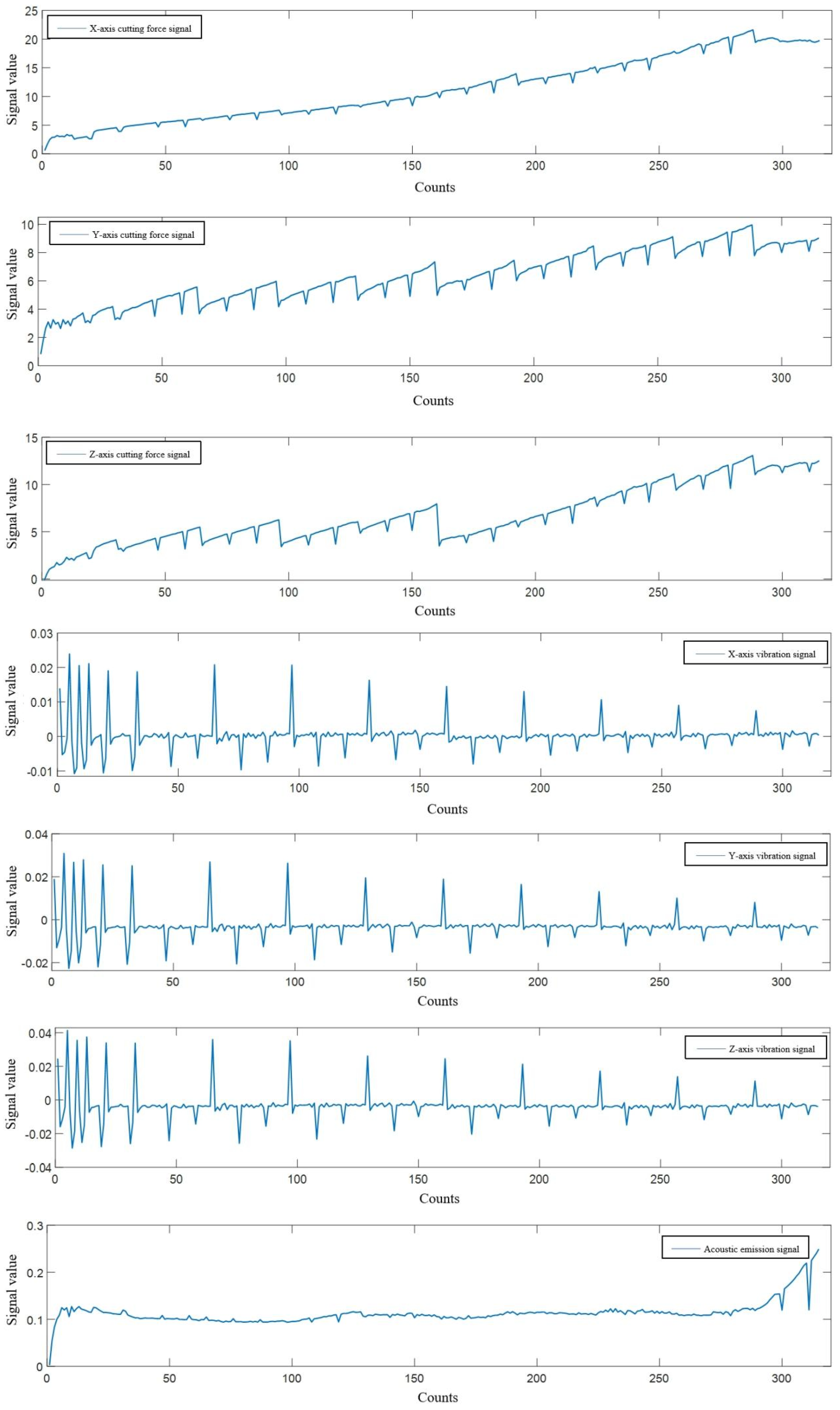
Each milling cutter (C1, C4, C6) has 315 samples covering its entire lifecycle, from initial use to end of life. Each sample contains extensive sensor signal data and corresponding wear value records. For example, the seven signals at the 33rd sample point of C6 (X-axis force, Y-axis force, Z-axis force, X-axis vibration, Y-axis vibration, Z-axis vibration, and acoustic emission signals) are visualized in Figure 2.5, showcasing sensor signal changes. Figure 2.6 illustrates the correspondence between the 7 signals and wear values of C1. Visualizing this relationship by pass number (Figure 2.7) shows the cutting force signal’s continuous increase with tool wear. The wear curve indicates three stages in the tool’s lifecycle, aligning with the described wear process.

Figure 2.5. 7 Signals of The 33rd Sample Point of C6 Milling Cutter.

Figure 2.5. 7 Signals of The 33rd Sample Point of C6 Milling Cutter.

Figure 2.6. C6 Milling Cutter 7 Types of Signals and Wear Value Correspondence Diagram.

Figure 2.6. C6 Milling Cutter 7 Types of Signals and Wear Value Correspondence Diagram.

Figure 2.7. C6 Milling Cutter Full Lifecycle 7 Types of Signals and Wear Values Curves.

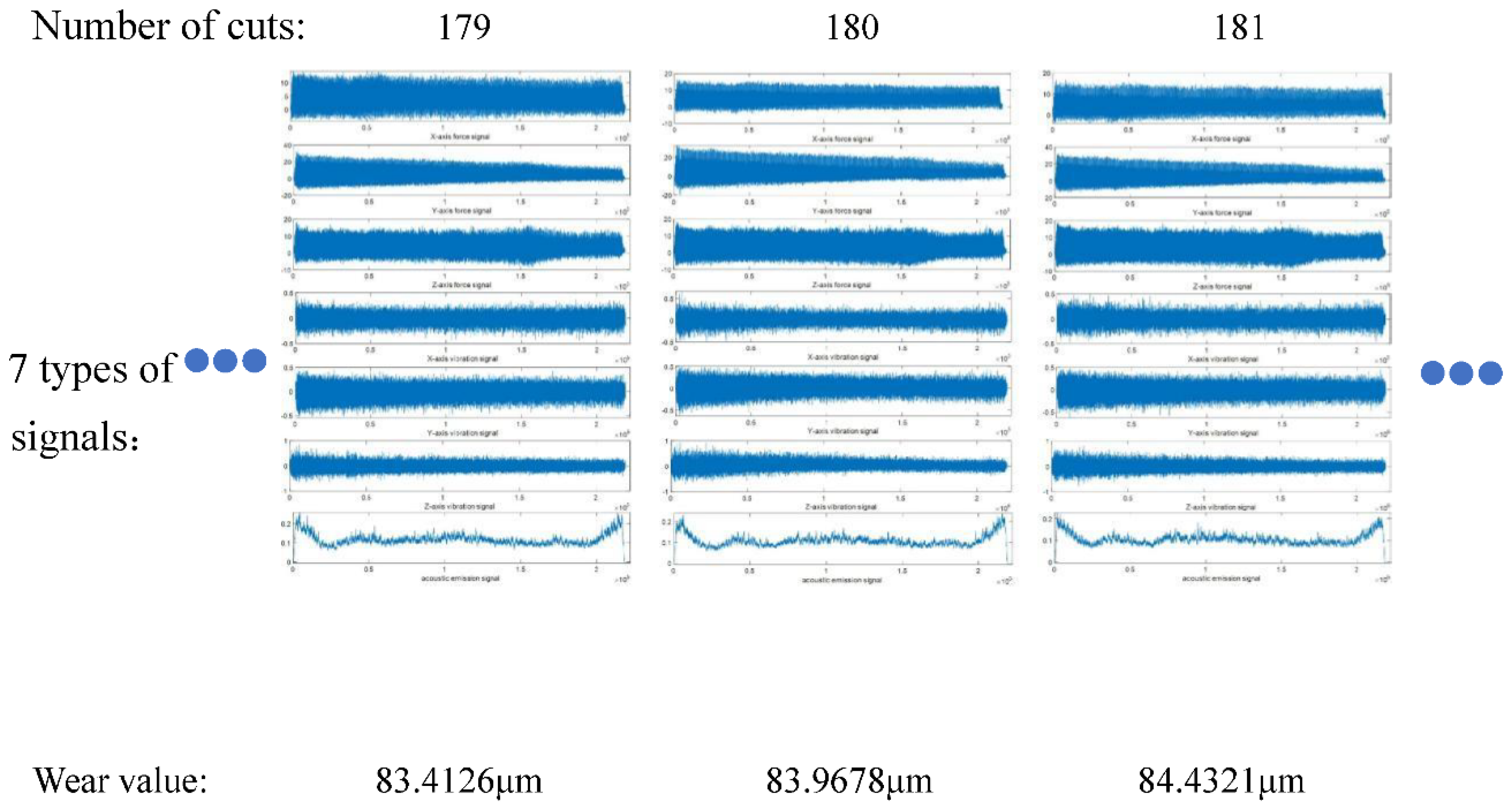
Figure 2.7. C6 Milling Cutter Full Lifecycle 7 Types of Signals and Wear Values Curves.

2.3. Preprocessing of Sensor Signal Data

The sensor signal data preprocessing in this article is mainly divided into two categories: defect data processing and noise data processing.

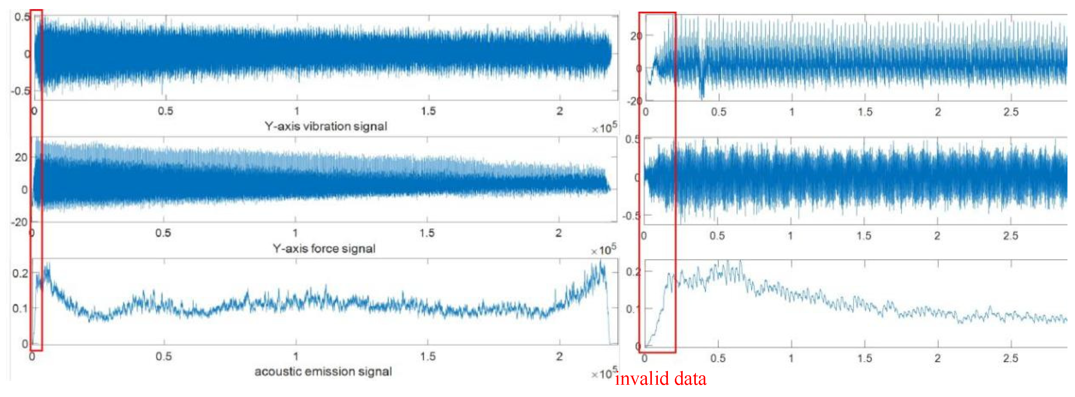
In this dataset, by sampling and visualizing signal data samples, it can be found that data defects mainly include invalid data and abnormal data, as shown in Figure 2.8. The invalid data specifically includes invalid data for cutting in and invalid data for cutting out, and abnormal data refers to jumping values caused by certain reasons. Therefore, the data preprocessing techniques involved generally include invalid value and outlier handling, etc. The schematic diagram of data defects is shown in Figure 2.9.

Figure 2.8. Data Defect Category.

Figure 2.8. Data Defect Category.

Figure 2.9. Data Defect Diagram.

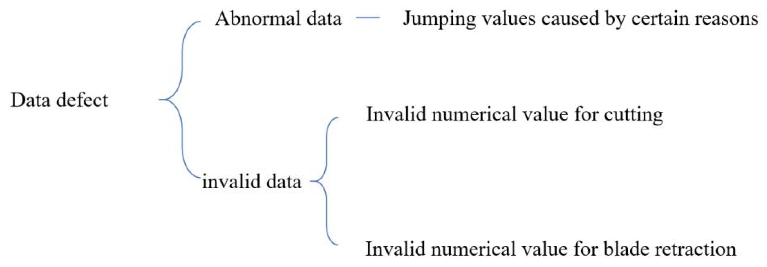
Figure 2.9. Data Defect Diagram.

After the above preprocessing, the sensor signals can meet the needs of the dataset. However, in actual processing, the collected sensor signals are mixed with noise interference due to the influence of the processing environment and machine vibration [55].If the original signal with noise is directly used as the input for feature extraction in the model, it will be difficult to extract more effective information, which seriously affects the recognition and prediction accuracy of the model in the future. For non-stationary signals, this paper adopts wavelet denoising as one of the commonly used denoising methods [56] Process it.

2.3.1. Invalid Value Handling

The processing of invalid value data can be divided into two types based on the number of data samples in different industrial production applications.

(1) Smooth interpolation filling

For data that is difficult to collect in actual processing and has a small sample size, curve fitting can be performed on existing samples by using smooth interpolation to fill in and generate more samples to replace invalid data. Specific methods include Lagrange interpolation.

(2) Directly delete

Due to the ease of obtaining data in some processing and production processes, the sample size is large enough, and there are relatively few invalid data. For such data samples, the invalid data can be directly deleted.

Due to the high frequency of experimental data collection, there are also more data points collected during the milling process, with each sample containing over 200000 data points. Visualization reveals that there are fewer invalid data points, so direct deletion can be used.

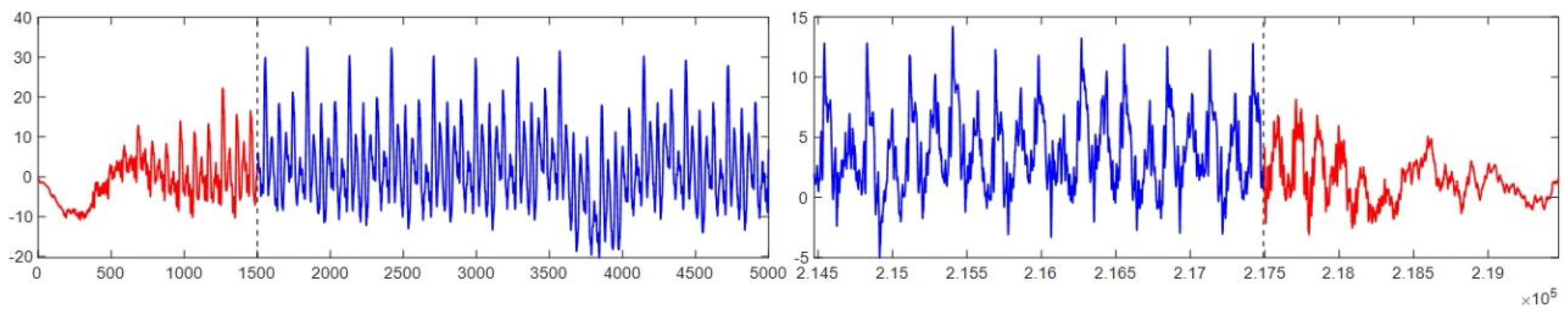
For determining deletion points, a third quartile method (Q3) can be used. Arrange sample data in ascending order, dividing into four equal parts, with the third quartile (Q3) as the localization point. Calculate Q3 and compare it with the critical value for ineffective data during cutting and retracting. Start from the first data value, comparing it sequentially with Q3 until the first value > Q3 is found, marking the deletion location. Data from the initial value to this point is invalid during cutting, and from this point to the final value is invalid during retracting. Figure 2.10 magnifies the Z-axis cutting force signal of the 225th sample in C1. The data range is (-40, 60), with 75% being 30. The Q3 method truncates data as shown: the blue solid line represents truncated data, and the red solid line represents deletable invalid data during feed and retract.

Figure 2.10. Q3 Cutting Method with Truncated Progression - Invalid Data Illustration.

Figure 2.10. Q3 Cutting Method with Truncated Progression - Invalid Data Illustration.

2.3.2. Outlier Handling

Outliers in industrial environments are categorized into point, fluctuation, collective outliers, and obvious noise signals. Abnormal data typically shows sudden amplitude jumps, creating extreme values. Effective methods to detect and process such data without affecting normal data are needed. This study employs hampel filtering, a median filtering method using sliding windows, as detailed in Table 2.5.

Table 2.5. Hample filtering for handling outliers.

Step	Describe
1:	Set the number of samples k on both sides of the sample, then the window size is 2k+1, and set the upper and lower bound coefficients nδ.
2:	Calculate the local standard deviation xδ of each sample based on sliding window, Local estimation median xm.
3:	Calculate the upper and lower bounds of outliers for the sample:
	Outlier upper bound: upbound = xm + nδ × xδ
	Outlier lower bound: downbound = xm - nδ × xδ
4:	If the sample value is greater than or less than the upper bound of the outlier, use the estimated median xm replace the sample.

Table 2.5. Hample filtering for handling outliers.

Step	Describe
1:	Set the number of samples k on both sides of the sample, then the window size is 2k+1, and set the upper and lower bound coefficients nδ.
2:	Calculate the local standard deviation xδ of each sample based on sliding window, Local estimation median xm.
3:	Calculate the upper and lower bounds of outliers for the sample:
	Outlier upper bound: upbound = xm + nδ × xδ
	Outlier lower bound: downbound = xm - nδ × xδ
4:	If the sample value is greater than or less than the upper bound of the outlier, use the estimated median xm replace the sample.

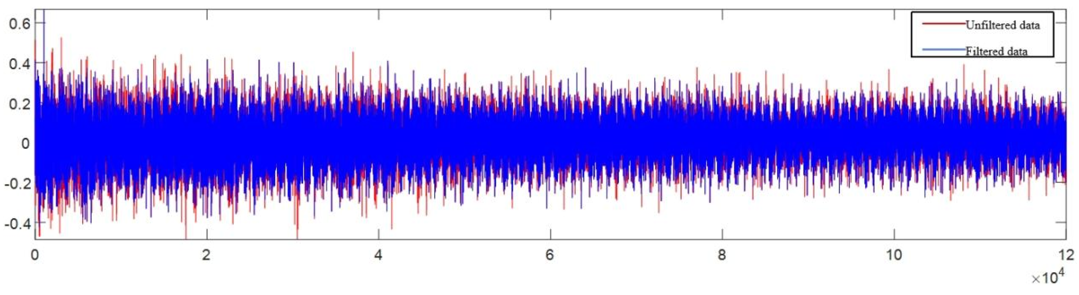
set up k = 4000, n_δ = 3.The final filtering effect comparison is shown in Figure 2.11, where the red dashed line represents data containing abrupt outliers, and the blue solid line represents data after replacing outliers.It can be seen that after Hampel filtering, the abnormal value of Z Vibration in sample 033 of the C6 dataset was replaced with a more normal value, while other data were not affected, the curve was smoother, and the abnormal data points were not obvious. The blue replaced data generally covered the data before the red replacement.

Figure 2.11. Hampel Filter Anomaly Replacement Illustration.

Figure 2.11. Hampel Filter Anomaly Replacement Illustration.

2.3.3. Wavelet Denoising

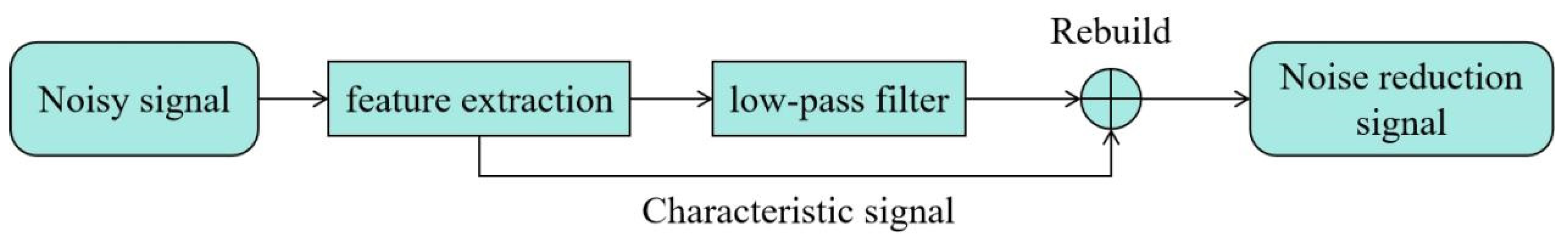
This article adopts wavelet threshold denoising [57],the main idea is to divide the signal and noise by setting an appropriate threshold and setting the noise to 0 to achieve the goal of removal. As shown in Figure 2.12, this method can denoise the signal through low-pass filtering while preserving the extracted features, making it superior to traditional denoising methods.

Figure 2.12. Principle of Wavelet Denoising.

Figure 2.12. Principle of Wavelet Denoising.

The process of wavelet threshold denoising is shown in Figure 2.13, where the selection of wavelet basis, threshold, and threshold function can be carried out according to the following process.

(1) The wavelet basis function adopts “sym8” with 5 layers;

(2) The threshold selection adopts the following formula:

$$T={\displaystyle \frac{M(\left|{\mathrm{cD}}_1\right|)}{0.6745}}\sqrt{2\ln N}$$

(2.1)

In the formula cD₁—Detail coefficients of the first layer decomposition;

N—Length;

M—Calculate median.

(3) The threshold function adopts a compromise between soft and hard thresholds, expressed as:

$$\mathrm{sgn}=\left\{\begin{array}{c}1, x>0\\ 0, x=0\\ -1, x<0\end{array}\right.$$

(2.2)

In the formula, x represents the signal data value.

Figure 2.13. Wavelet Threshold Denoising Process.

Figure 2.13. Wavelet Threshold Denoising Process.

To verify the quality of sensor timing data after wavelet denoising, the signal-to-noise ratio (SNR) is used to determine the denoised results. The formula for calculating SNR is shown in (2.3):

$$SNR=10\lg \left({\displaystyle \frac{P_{\mathrm{s}}}{P_n}}\right)$$

(2.3)

The SNR value before denoising is 9.8, and after denoising it is 17.6. The denoised signal is smoother, and the SNR of the signal is nearly doubled, proving that the wavelet threshold denoising used can remove noise from the signal.

For the cutting force signal and vibration signal of the first cutting of C6 in the dataset, frequency spectrum analysis was performed separately, as shown in Figure 2.14 and Figure 2.15.

Figure 2.14. Spectral Analysis of Cutting Force Signal.

Figure 2.14. Spectral Analysis of Cutting Force Signal.

Figure 2.15. Spectral Analysis of Vibration Signals.

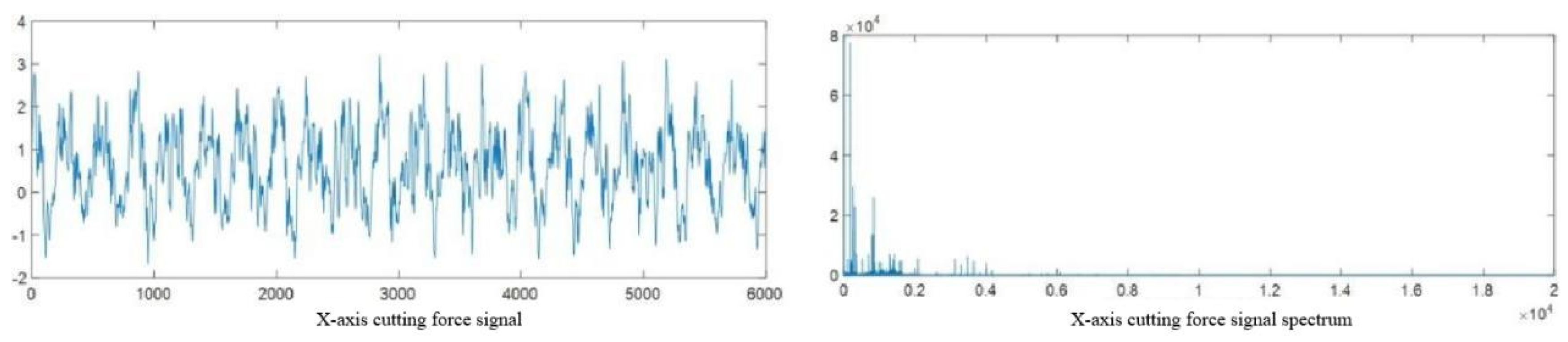
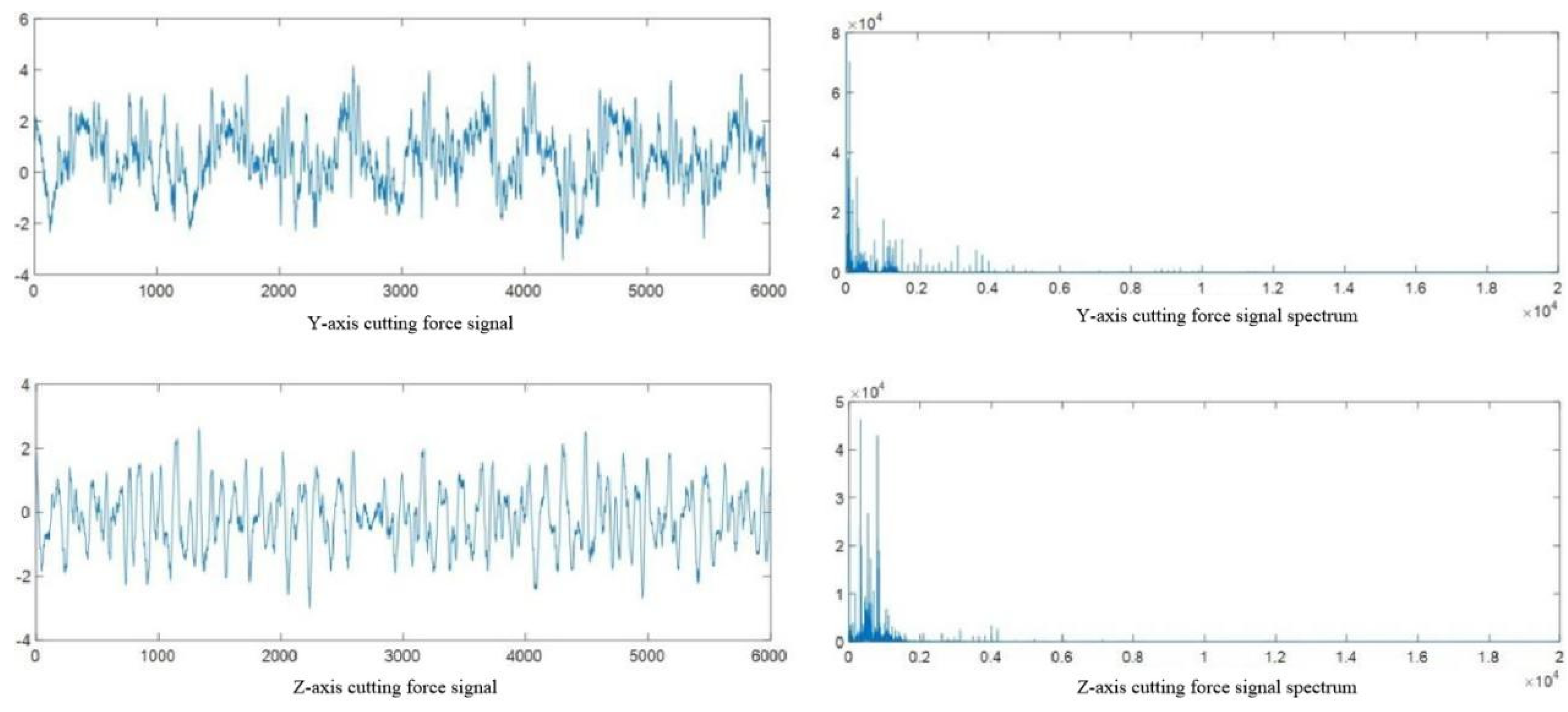
Figure 2.15. Spectral Analysis of Vibration Signals.

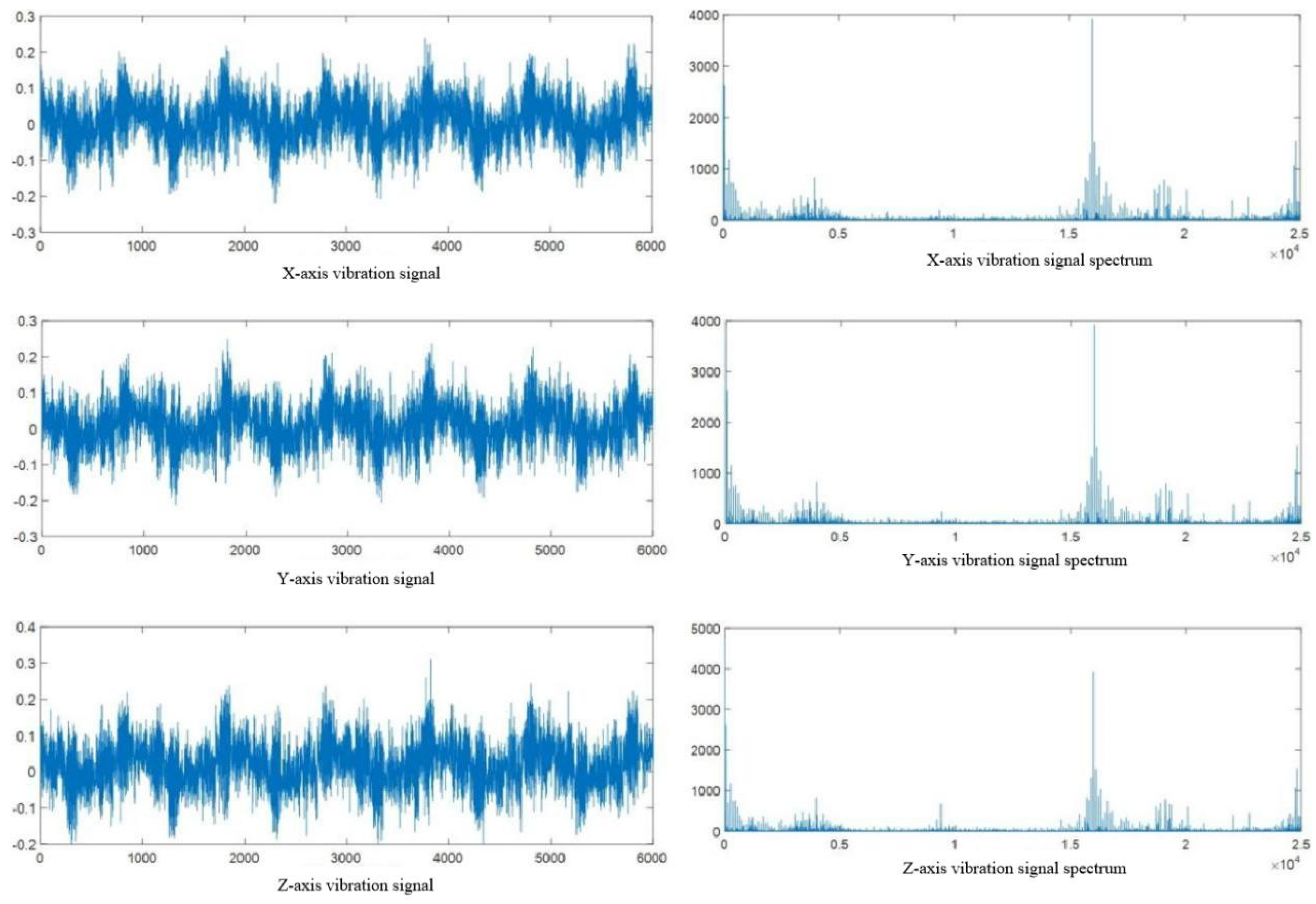
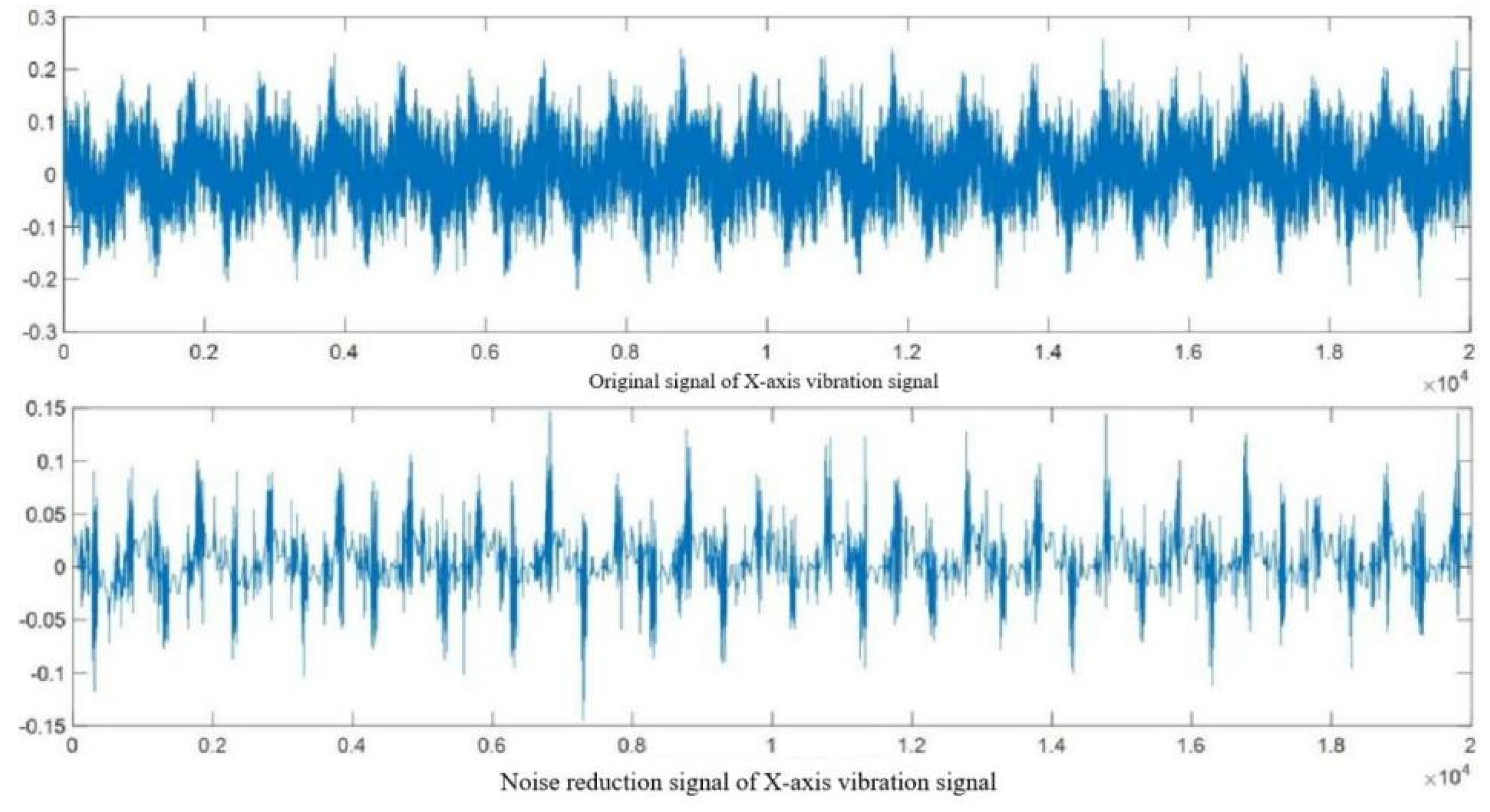
Figures 2.14 and 2.15 show that the original cutting force signal has minimal noise, with its frequency spectrum mainly in the 0-5000Hz low-frequency range without high-frequency noise interference, thus requiring no noise reduction. Conversely, the vibration signal is heavily noise-affected, particularly in the 0-10000Hz low-frequency and 15000-25000Hz high-frequency ranges with significant amplitude, signifying substantial noise interference. Therefore, wavelet threshold denoising is applied to the vibration signals in the three directions (X, Y, Z) to mitigate noise interference, as illustrated in Figure 2.16 for the X-axis vibration signal.

The analysis and processing of invalid data, outlier localization analysis, and data filtering on the raw data in the tool wear dataset have obtained relatively accurate and high-quality data, laying the foundation for establishing a state monitoring and life prediction model in the next step.

Figure 2.16. The Original and Denoised Vibration Signals In The X-axis Direction.

Figure 2.16. The Original and Denoised Vibration Signals In The X-axis Direction.

3.1. CNN Informer and Encoding Decoding Framework

The multi-step prediction process for tool wear based on Informer is shown in Figure 3.1.

Figure 3.1. Flowchart of Multi-step Tool Wear Prediction Based on CNN-Informer.

Figure 3.1. Flowchart of Multi-step Tool Wear Prediction Based on CNN-Informer.

This chapter mainly designs the Informer structure for wear monitoring, and based on the encoding decoding framework, improves the intermediate layer to achieve wear prediction. The key model structures include Informer and encoding decoding framework, so this section mainly introduces and analyzes them.

3.1.1. The Principle of Convolutional Neural Network

CNN, inspired by biological visual mechanisms, is a widely used deep learning architecture. Through convolution operations, neurons respond within their receptive fields, reducing parameters and complexity, enhancing training efficiency. Design of convolutional kernels allows feature extraction and learning, minimizing manual extraction and enabling deeper feature mining. Pooling layers and nonlinear activation functions further improve generalization and robustness by reducing data dimensions and capturing complex nonlinear relationships. CNN showcases strong potential in image recognition, video analysis, and NLP, automating pattern discovery and significantly enhancing performance in complex tasks. It has achieved notable results in image classification, object detection, video understanding, and biomedical imaging [59].

The typical structure of a convolutional neural network is shown in Figure 3.2, which mainly includes the following structures:

(1) Convolutional Layer

As the core of convolutional neural networks, convolutional layers are generally composed of multiple convolutional kernels. Convolutional kernels extract features from input data through convolution operations, and as the number of convolution layers gradually increases, the extracted features become increasingly abstract. The expression for convolution operation is shown in equation (3.2):

$${\mathrm{x}}_j^l=f({\displaystyle \sum _{i\in M_j}{W}_{ij}^l}\ast x_i^{l-1}+b_j^l)$$

(3.1)

Figure 3.2. Typical Convolutional Neural Network Structure.

Figure 3.2. Typical Convolutional Neural Network Structure.

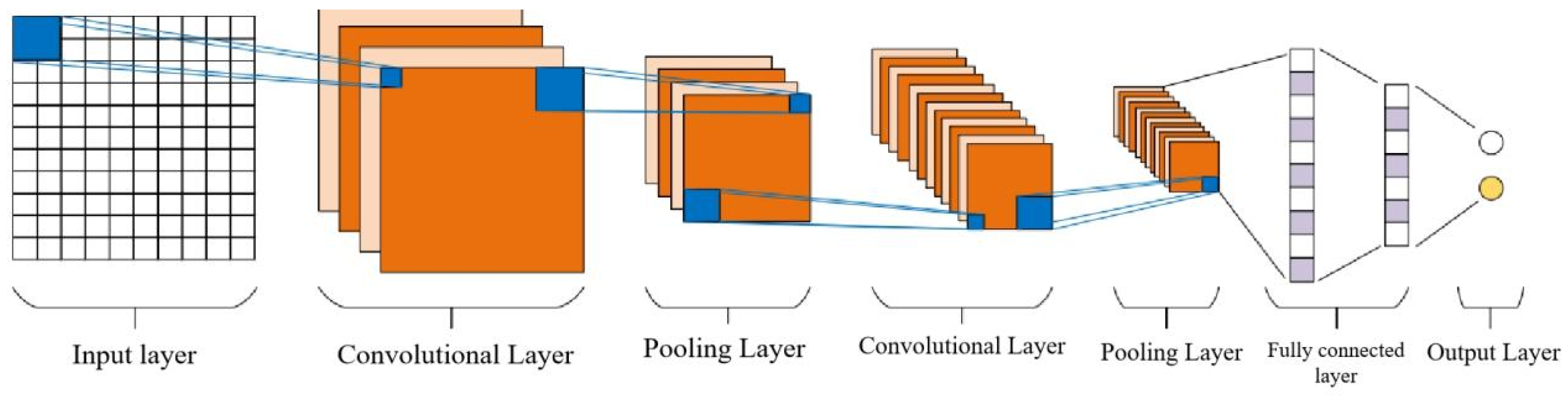
Among them, ${\mathrm{x}}_j^l$ represents the jth feature image of the l-th layer, $W_{\mathrm{ij}}^{\mathrm{l}}$ represents the weight between the j-th feature image in the l-th layer and the i-th feature image in the l-1 layer, ${\mathrm{b}}_{\mathrm{j}}^{\mathrm{l}}$ represents its corresponding bias, and f represents the activation function, * represents convolution operation, $M_{\mathrm{j}}$ represents the set of input graphs.From the above equation, it can be seen that convolution operations are mainly composed of linear operations and nonlinear operations. Among them, linear operations are mainly affected by feature weights and biases, and weight and sum some features of the feature image. Nonlinear operations are based on activation functions to apply influence, so activation functions usually have a significant impact on the performance of convolutional layers. Common activation functions include sigmoid (equation 3.2), tanh (equation 3.3), and relu (equation 3.4). Due to their inherent characteristics, sigmoid and tanh may exhibit overly flat output performance when the input data is very large or very small, which can easily cause gradient vanishing during the training process and ultimately lead to convergence difficulties for deep learning. Therefore, the convolutional layers of convolutional neural networks generally consider using ReLU as their activation function.

$$f(x)={\displaystyle \frac{1}{1+e^{-x}}}$$

(3.2)

$$g(x)={\displaystyle \frac{e^x-e^{-x}}{e^x+e^{-x}}}$$

(3.3)

$$h(x)=\max (0,x)$$

(3.4)

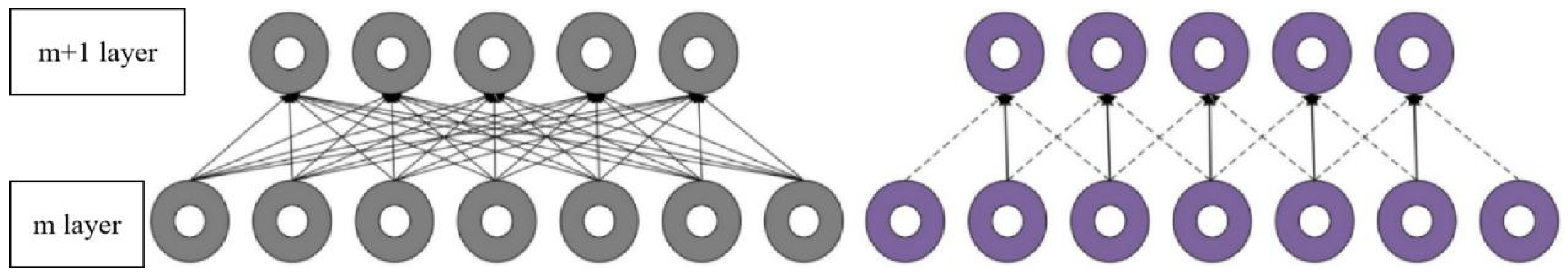
Convolutional layer neurons are sparsely connected, facilitating weight sharing and sparse connections, as depicted in Figure 3.3. Sparse connections limit neuron receptive fields but, in deep networks, deeper neurons still interact with input data. This maintains robustness while reducing model complexity. Weight sharing reduces parameter learning and storage, enhancing computational efficiency by calculating weights on fixed-size kernels.

Figure 3.3. The Difference Between Full-Connected and Non-Fully Connected.

Figure 3.3. The Difference Between Full-Connected and Non-Fully Connected.

(2) Pooling layer

The pooling layer usually follows the convolutional layer and aggregates the features of adjacent regions in the feature map based on convolution operations, achieving downsampling of the original features. The pooling layer can reduce the size of feature maps while ensuring feature validity, thereby accelerating the training rate of the model. The pooling calculation is shown in equation (3.5):

$${\mathrm{x}}_j^l=f({\beta }_j^{l}down(x_j^{l-1})+b_j^l)$$

(3.5)

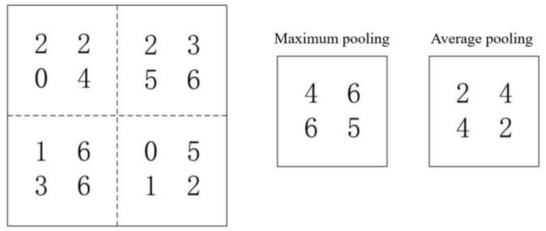
Among them, down (.) is a pooling function, and each feature map has its own multiplier bias β and additional bias b. The pooling layer mainly includes three pooling methods: max pooling, average pooling, and random pooling. Maximum pooling eliminates some minor features by retaining the maximum value of features within the pooling area, but this may amplify the noise in the features and reduce the generalization ability of the model. Average pooling achieves comprehensive consideration of all features in the pooled area by arithmetic averaging and recording the mean, but it also reduces the strength of typical features in the area. Random pooling uses a random selection method to preserve a feature within the pooling area, and it is precisely the randomness introduced by this method that improves the robustness of the model. As shown in Figure 3.4, the effects of max pooling and average pooling on feature maps are demonstrated.

Figure 3.4. Max Pooling and Average Pooling.

Figure 3.4. Max Pooling and Average Pooling.

(3) Fully connected layer

The combination of convolutional layers and pooling layers forms the low hidden layer of a convolutional neural network. The network completes the extraction of local features in the low hidden layer, and then needs to integrate them into global features to achieve comprehensive analysis of global features. The fully connected layer is usually set at the end of the convolutional neural network to summarize and synthesize the previously extracted local features. All neurons in the fully connected layer will be connected to all neurons in the previous layer, including both linear and nonlinear operations. The calculation formula is shown in equation (3.6):

$$x^l=f(w^l{x}^{l-1}+b^l)$$

(3.6)

Among them, $x^{l-1}$ is the output feature map of layer l-1, $w^l$ is the l-layer feature map $x^l$ connect to $x^{l-1}$ the weight, $b^l$A is the bias coefficient of layer l.

(4) Output layer

The output layer essentially belongs to the fully connected layer, which serves as the end of the entire network to calculate the final output result. The activation functions of the output layer are classified into multiple categories based on their different purposes. For regression problems, the results can be directly calculated and output; For classification problems, softmax is generally used as the activation function (Equation 3.7), and then the classification results are calculated.

$$y^i={\displaystyle \frac{e^{z_i}}{{\displaystyle \sum _{j=1}^C{e}^{z_j}}}}$$

(3.7)

Among them, $Z_i$ is the output of the previous unit received by the classifier, i represents the category index of the classifier, and C is the number of all categories. $y^i$ represents the ratio of the index of the current element to the sum of the indices of all elements in the classifier.The softmax function can be used to convert the numerical values output by a multi class model into the relative probabilities of each class.

3.1.2. Feature Extraction Based on One-Dimensional Convolution Kernel

In recent years, deep convolutional networks have achieved remarkable success in image processing, sparking interest in applying Convolutional Neural Networks (CNNs) to sensor signal processing. Sensor signals, typically one-dimensional (1D) data like time series, differ from traditional 2D image data. Standard CNNs with 2D convolution kernels aren’t suitable, necessitating the introduction of 1D CNNs. These networks efficiently process time series signals using 1D convolution kernels for feature extraction. With a simpler structure than 2D CNNs, 1D CNNs directly accommodate 1D data characteristics, reducing complexity. Studies show that 1D CNNs excel in temporal signal analysis, automatically extracting features and eliminating the need for manual feature engineering. They also extract higher-level abstract features through layered convolution, often elusive to traditional methods. By stacking multiple convolution layers, 1D CNNs capture temporal dependencies and local signal features, crucial for tasks like signal classification, regression, or anomaly detection. This approach not only simplifies multi-source information fusion but also extracts abstract features beyond traditional methods’ reach. Furthermore, 1D CNNs integrate easily with other modules like Recurrent Neural Networks (RNNs), bolstering their complex temporal data processing capabilities.

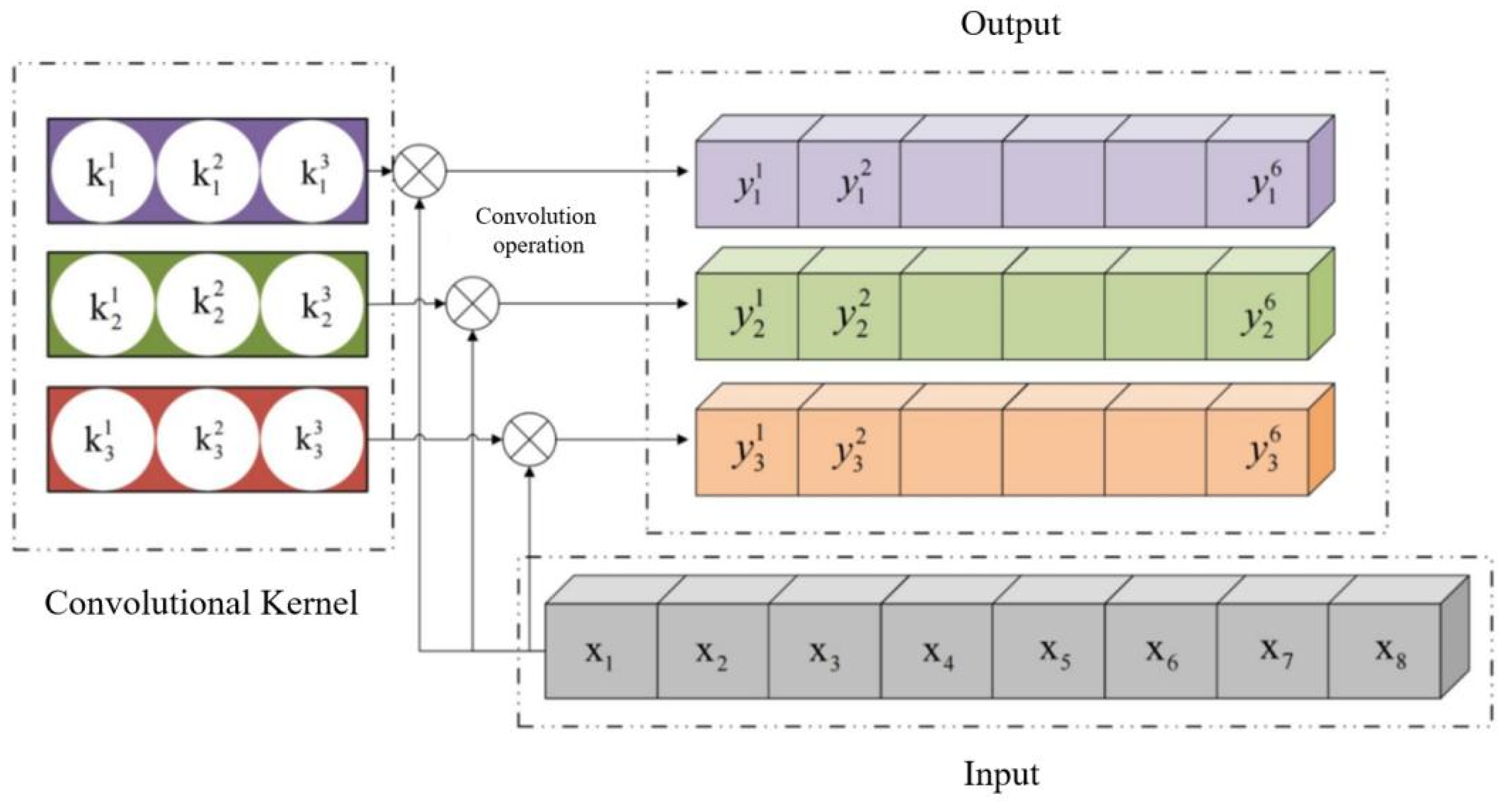
The schematic diagram of one-dimensional convolution operation is shown in Figure 3.5. This convolutional layer contains three convolutional kernels, with a kernel size of 3. Each kernel will traverse the input signal once and perform a convolution operation to obtain the feature output after the convolution operation. Taking the first convolution kernel in Figure 3.5 as an example, it has three weights $({\mathrm{k}}_1^1,k_1^2,k_1^3)$, When using convolution kernels for convolution operations, each weight in the kernel is sequentially multiplied and summed with the corresponding neuron in the convolved region, and the corresponding activation function is applied to the summed value to obtain the output value $y_1^1$. Subsequently, the convolution kernel slides through the entire input signal with a step size of 1 and repeats the previous convolution operation until the kernel traverses the entire input signal. At this point, the complete output of the first convolution kernel, $(y_1^1,y_1^2,\cdot \cdot \cdot ,y_1^6)$, can be obtained.

Figure 3.5. The Convolution Calculation Process of One-Dimensional Convolution Kernel.

Figure 3.5. The Convolution Calculation Process of One-Dimensional Convolution Kernel.

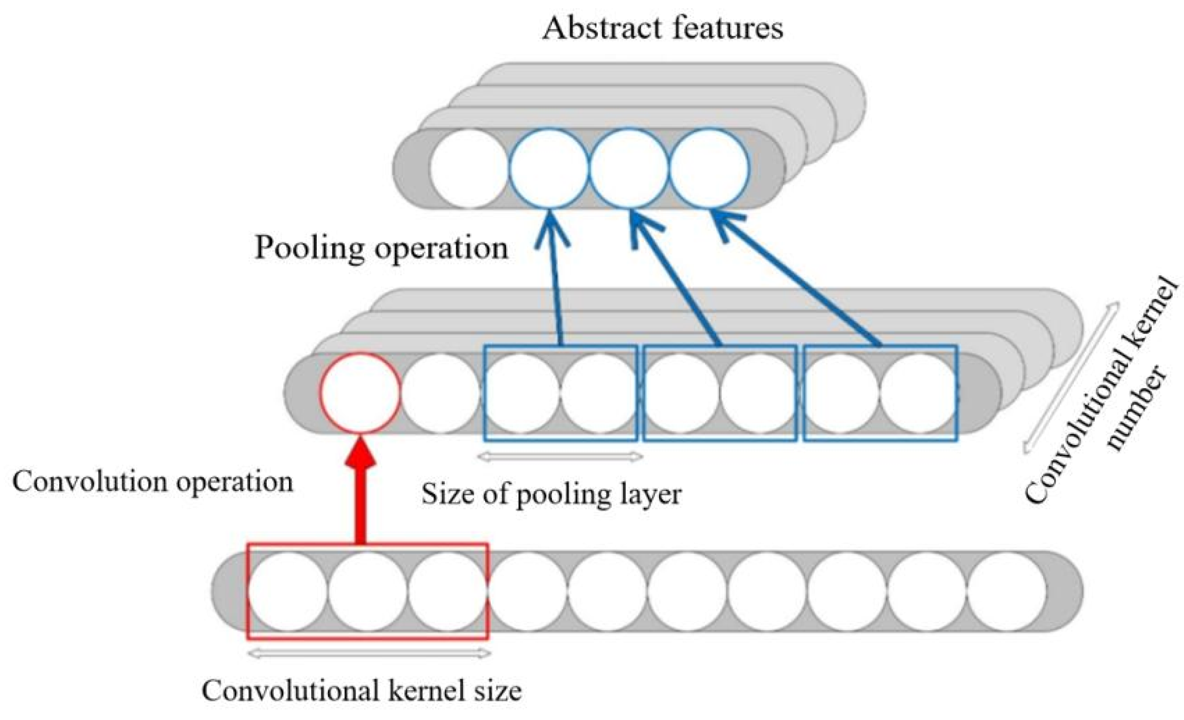
After convolution, a pooling operation is typically performed, as shown in Figure 3.6. Multiple 1D convolution kernels extract multi-dimensional features from the input, while pooling reduces feature map size and accelerates subsequent feature extraction. Through the stacking of multiple convolutional and pooling layers, feature maps derived from the original signal are abstracted from shallow to deep, ultimately yielding abstract features representing the input vector.

Figure 3.6. Combination of Convolution and Pooling Operations.

Figure 3.6. Combination of Convolution and Pooling Operations.

3.1.3. The Principle of Informer Model

Before introducing the Informer model, let’s briefly talk about the shortcomings of its predecessor, the Transformer model.The Transformer mechanism was proposed by Vaswani et al [61]. in 2017, and is a neural network model based on attention mechanism proposed by the research team for machine translation tasks, namely the Transformer model.The Transformer model introduces a mechanism called “self attention mechanism” to weight and combine information from different positions when processing input sequences, thereby achieving parallel processing and long-range dependency modeling, greatly improving the efficiency and performance of sequence data processing. However, Transformer has several serious issues, such as not being directly applicable to long-term time series prediction problems, such as quadratic time complexity, high memory usage, and inherent limitations of encoder decoder architecture, with certain restrictions on sequence length, and so on [62].

Position encoding is an important part of Transformer, which is divided into absolute position encoding and relative position encoding. Currently, relative position encoding operates on the attention matrix before softmax, which theoretically has a drawback. The attention matrix with relative positional information is a probability matrix, where the sum of each row is equal to 1. For Transformers, self attention enables interaction between tokens, where the same input indicates that each $V_{\mathrm{t}-1}$ is the same.That is to say, the difference between the collected data is very small in a short period of time, and due to accuracy issues, the output results of each position of the model are always the same or extremely similar data. Transformers also have the drawbacks of high computational complexity and long training time. Compared with CNN and RNN, Transformer has weaker ability to obtain local information [63].

The Informer mechanism is an innovative approach for time series prediction, emerging around 2017 [64]. Researchers began experimenting with self-attention mechanisms for time series data processing, recognizing the Transformer’s limitations with fixed-size memory, which hinders long sequence handling and remote feature capturing. To address this, Zhou [65] proposed Informer, an efficient model that splits sequences into varying-length subsequences via a hierarchical mechanism, dynamically adjusting processing based on contextual sequence length to better manage long sequences. Compared to Transformers, Informer excels in sequence modeling tasks, especially in predicting future time steps, by better processing temporal information, capturing long-term dependencies, and forecasting future trends [66].

The Informer model based on Transformer design has the following significant features:

(1) A sparse self attention mechanism that can achieve zero time and space complexity (LlogL), with lower complexity than traditional self attention mechanisms.

(2) The optimized multi head attention mechanism highlights dominant attention by halving the input of cascaded layers and effectively handles excessively long input sequences, improving the model’s ability to focus on various regions.

(3) A Transformer based generative decoder performs a forward operation on long time series instead of a step-by-step approach for prediction, greatly improving the inference speed of long sequence prediction. The other features are basically similar to Transformer and will not be further elaborated. The main structure of the Informer mechanism has been redrawn here, as shown in Figure 3.7.

Figure 3.7. Schematic Diagram of Informer Model Mechanism.

Figure 3.7. Schematic Diagram of Informer Model Mechanism.

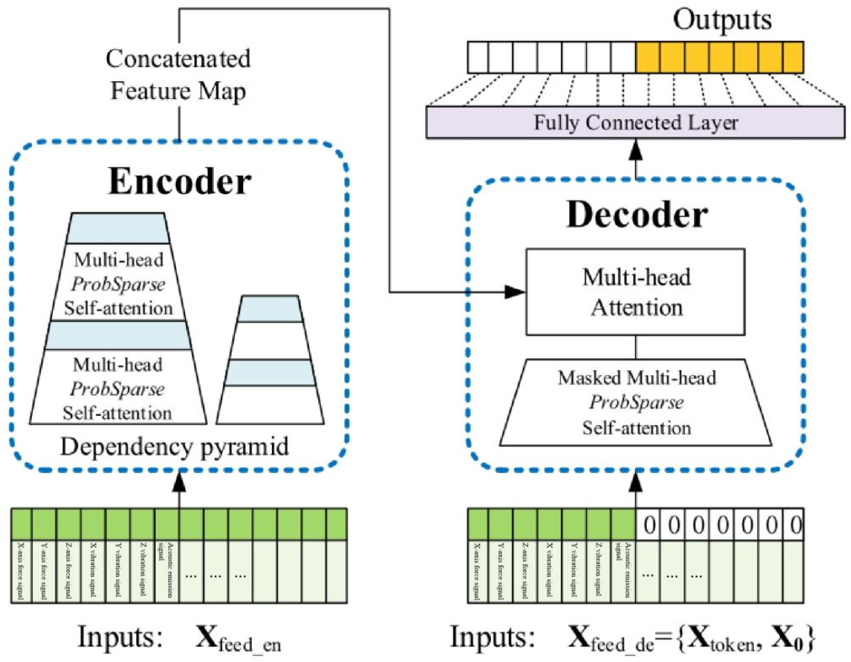
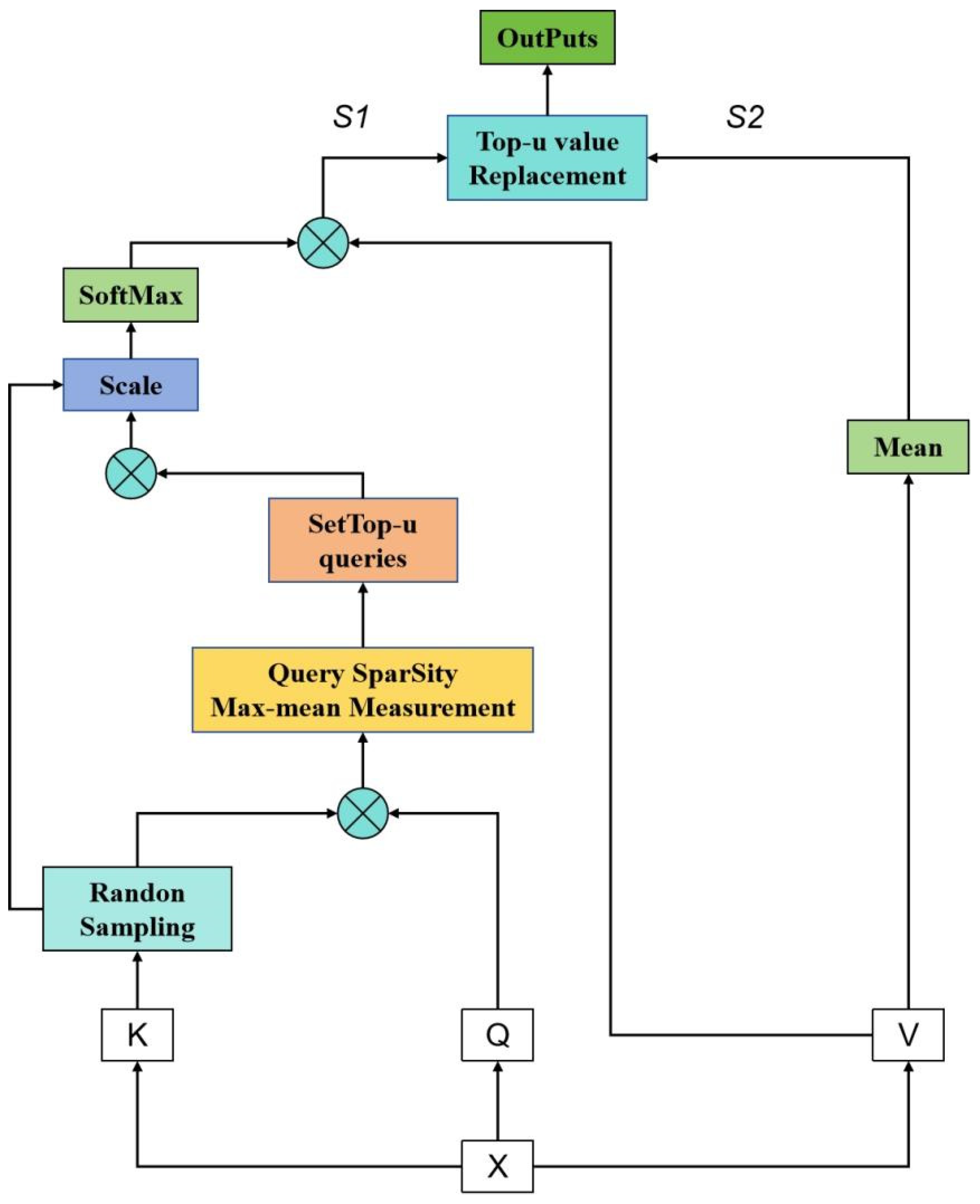
The Informer network consists of two main parts: an encoder and a decoder. In Figure 3.7, the encoder extracts a large number of long sequences $X_{\mathrm{en}}$(green series) from the input, and the self attention blocks are ProbSparses, which extract dominant attention and reduce network size.The decoder receives a long sequence input $X_{\mathrm{token}}$ (Green part before element 0),The filling element for 0 is $X_0$;The connected feature maps and attention combinations are fused to immediately predict long sequence outputs (yellow series). In the prediction of milling cutter wear, Informer adds position encoding to the data input to ensure that the model can capture the correct order of the input sequence.Location encoding is divided into Local Time Stamp and Global Time Stamp. time series $[X_t,\cdots ,X_{t+i},\cdots ,X_T]$,Using sensor signal data features as inputs to the Informer network, the temporal correlation $[X_t,\cdots ,X_{t+i},\cdots ,X_T]$ of the time series by using positional encoding, namely local timestamps and global timestamps, the local and global backward and forward temporal positional relationships of time series can be fully utilized [67].

By utilizing Informer’s multi head attention mechanism, attention is focused on prominent data features to obtain long-term dependencies of evaluation indicators in time series. The decoder input consists of two parts, one is the implicit intermediate feature data about sensor signal risk assessment indicators output by the encoder, and the other part requires the placement of evaluation indicators for predicting milling cutter wear, in order to use predicted 0 occupancy at the input and add masking mechanisms. The data is connected to the multi head attention mechanism, and then connected to the fully connected layer output to achieve the prediction of tool wear. After the encoding step, the input data entering the encoder layer can be obtained, as shown in formula 3.8.

$$X\prime =X+positionalEncoding(X)$$

(3.8)

Informer introduced ProbSparse, which first calculates the KL divergence between the i-th query and the uniformly distributed query to obtain the difference, and then calculates the sparsity score. The calculation formula for KL divergence is shown in 3.9.

$$D_{KL}(P‖Q)={\displaystyle {\sum }_{i}P(i)\log \frac{P(i)}{Q(i)}}$$

(3.9)

Among them, P (x) represents the probability distribution of the i-th query, and Q (x) represents the probability distribution of uniformly distributed queries. KL divergence measures the difference between two probability distributions, with larger values indicating that the two distributions are less similar.

Based on the above, the sparse attention mechanism ProbSparse is introduced, and the formula is shown in 3.10.

$$ProSparse(Q)={\displaystyle \frac{1}{N}}{\displaystyle {\sum }_{i}Q(i)}\log {\displaystyle \frac{Q(i)}{1/N}}$$

(3.10)

The Informer encoder is an important component of this model, designed to analyze the input sensor signal data in depth and extract the time series dependence of milling cutter wear through two intricately designed identical operation stacks. Each stack integrates a multi head self attention mechanism, which can process multiple attention heads in parallel, allowing the model to capture multi-level and complex temporal dependencies in the data. In addition, in order to preserve the position information of the time series, the encoder introduces position encoding to ensure that the precise position of each data point on the time axis can be considered when analyzing sensor signals.

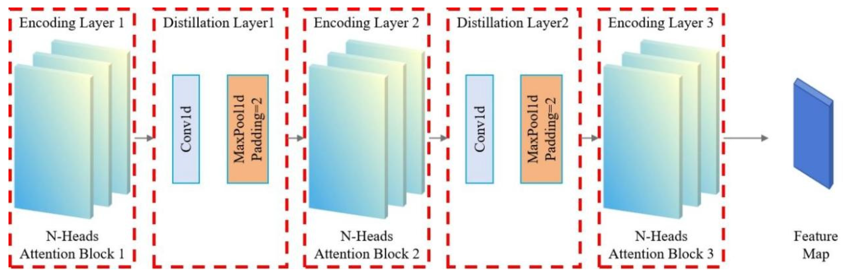
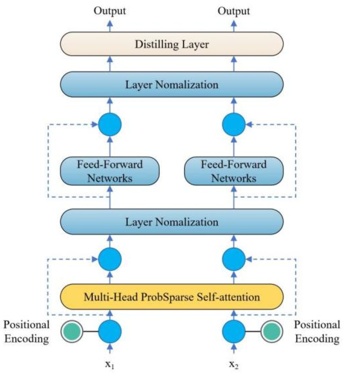
After the self-attention mechanism, the encoder employs a feedforward neural network (FFN) to extract complex patterns through nonlinear transformations on intermediate features. Residual connections and layer normalization enhance training stability and mitigate gradient issues. These technologies enable efficient long time series processing, mapping milling cutter wear information to sensor-reflecting intermediate features. These features underpin the decoder, enhancing milling cutter wear prediction accuracy, vital for industrial predictive maintenance and fault diagnosis, boosting production efficiency and equipment reliability. Informer excels in complex time series handling, shown in Figure 3.8. Stack 1 processes the full input sequence, while Stack 2 handles half, each comprising an encoding layer, distillation layer (including a multi-head probabilistic sparse self-attention layer, FFN, residual connections, and regularization), as detailed in formula 3.11.

The Distillation layer improves the robustness of the network and reduces the memory used by the network. The outputs of all stacks are concatenated to obtain the final hidden representation of the encoder, as shown in Figure 3.7. Among them, Sublayer is a multi head sparse self attention mechanism and forward neural network processing function, while LayerNorm is a regularization function.

$$O=LayerNorm(x+Sublayer(x))$$

(3.11)

Figure 3.8. Informer Encoder Stack Structure.

Figure 3.8. Informer Encoder Stack Structure.

3.1.4. Typical Self Attention Mechanism and Improved ProbSparse Self Attention Mechanism

(1) Typical self attention mechanism

A typical attention mechanism is a commonly used mechanism in deep learning to selectively focus on certain positions in an input sequence, thereby achieving weighted processing of different positions. The calculation formula is shown in 3.12.

$$Attention(Q,K,V)=soft\max ({\displaystyle \frac{Q{K}^T}{\sqrt{d_k}}})V$$

(3.12)

Calculating weights based on the relationships within the input sequence. In the self attention mechanism, the model calculates the dot product between the query vector (Q) and the key vector (K), and divides it by a scaling factor (usually the square root of the vector dimension) to obtain the weights. Then, by normalizing the weights through a softmax function, the weight distribution is obtained. Finally, multiply the weight distribution with the value vector (V) to obtain the weighted value vector as the final self attention representation. The self attention mechanism can automatically learn the weight distribution based on the dependency relationship between different positions, thus paying more attention to important position information in the encoding process.

(2) Improving the Prob Sparse self attention mechanism

In order to address the issues of self attention, Zhou et al. proposed an improved Probe Sparse self attention mechanism, whose structure is shown in Figure 3.9 [68].

Prob Sparse Self Attention is a variant of the attention mechanism in deep learning, introducing probabilistic sparsity to limit the attention weight matrix’s sparsity, reducing computational complexity and model parameters. It calculates the dot product between query (Q) and key (K) vectors, applies a softmax function to obtain the initial attention weights, then computes the KL divergence between Q and a uniform distribution to measure dispersion. This divergence penalizes overly concentrated attention weights. By calculating a sparsity score, the difference is scaled to obtain a corrected attention weight matrix. Finally, this matrix is multiplied with the value (V) vector to produce the weighted representation, serving as the final Prob Sparse Self Attention output.

Prob Sparse Self Attention reduces the density of the generated attention weight matrix by introducing probability sparsity, thereby reducing computational complexity and model parameters. This attention mechanism is particularly useful when dealing with long sequence data, as it can improve the computational efficiency and performance of the model. Meanwhile, Probe Sparse Self Attention can also flexibly control the sparsity of attention weights by adjusting the weights of sparsity scores, thus adapting to the needs of different tasks and model structures.

Figure 3.9. Prob-Sparse Self-attentive structure.

Figure 3.9. Prob-Sparse Self-attentive structure.

3.1.5. Optimization of Multi Head Attention Mechanism

The optimized multi-head attention enhances the attention layer’s performance by expanding focus areas and providing multiple ‘representation subspaces’. This allows learning from diverse subspaces. Figure 3.10 depicts the structure of the optimized multi-head self-attention module.

Figure 3.10. Multi-headed attention mechanism structure.

Figure 3.10. Multi-headed attention mechanism structure.

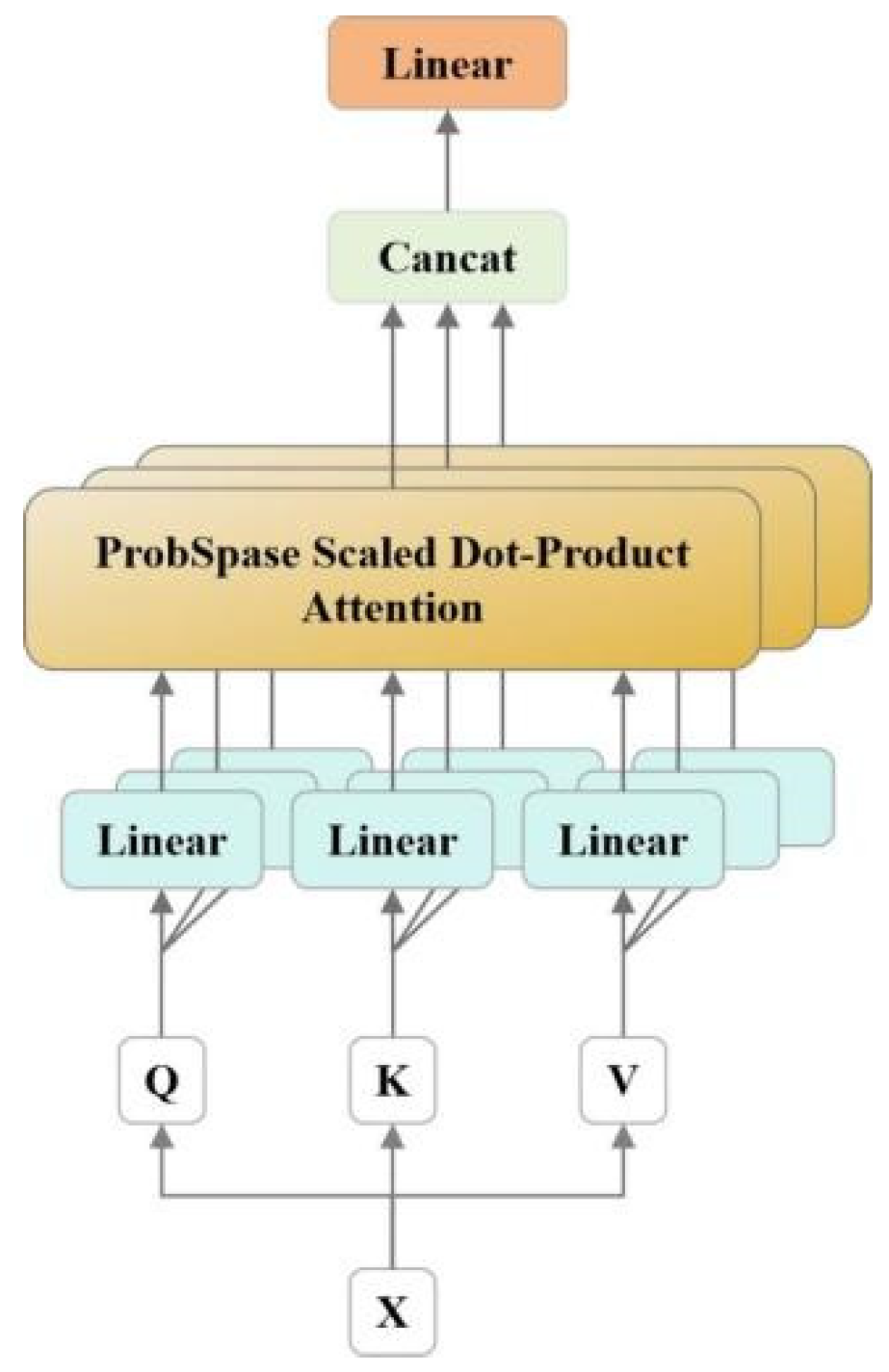
The Q, K, and V in the linear layer of the figure were initially applied to linear transformations. Then feed back the results of the linear transformation to the self attention layer. The output values are concatenated and then a linear transformation is applied to determine the final result. By using formulas 3.13 and 3.14, the following results can be obtained:

$$M\mathrm{u}lti-Head Attention\left(Q,K,V\right)=Concat(hea{d}_1,\dots ,hea{d}_h)W^O$$

(3.13)

The calculation formula for a single head is as follows:

$$headi=Attention(Q\ast WQi,K\ast WKi,V\ast VWVi)$$

(3.14)

3.1.6. Encoder and Decoder

(1) The encoder extracts robust long-term dependencies from long sequence inputs, which are shaped into a matrix. Figure 3.11 shows a schematic diagram of the encoder, and the decoder is similar to the encoder diagram and will not be repeated here.

The encoder is responsible for transforming the input sequence into an abstract representation that contains the semantic information of the input sequence. Encoders are typically composed of multiple layers, each containing multiple sub layers such as Self Attention mechanism, Feed Forward Neural Network, and multi head attention module.

Figure 3.11. Encoder and Decoder structure diagram.

Figure 3.11. Encoder and Decoder structure diagram.

(2) The decoder is responsible for converting the abstract representation output by the encoder into the target sequence. Its working process is similar to that of the encoder, but it usually includes additional attention mechanisms to handle the relationship between the encoder output and the target sequence [69].The working process of encoders and decoders is usually achieved through the combination of multiple layers and sub layers. Each layer can use different attention mechanisms, feedforward neural networks, etc. for information processing, gradually extracting semantic information from the input sequence and generating the output of the target sequence. The working process is shown in Figure 3.11. This encoder decoder structure has achieved significant performance improvements in many sequence data processing tasks.

3.1.7. Feedforward Network

A Feed Forward Network (FFN) is a fully connected feedforward neural network that is often used as part of attention mechanisms, such as in encoders and decoders. FFN typically consists of two fully connected layers, which introduce nonlinear transformations into the attention mechanism to increase the expressive power of the model. Specifically, FFN takes the output of the attention mechanism as input, processes it through two fully connected layers, and finally generates the output of the encoder or decoder. The calculation formula is shown in 3.15.

$$FFN(X)=\max (0,X{W}_1+b_1)W_2+b_2$$

(3.15)

In summary, X is the input vector, W1/W2 and b1/b2 are weight matrices and bias vectors of two fully connected layers, and Max(0, x) denotes the ReLU activation function. FFN introduces nonlinearity into the attention mechanism, enhancing model expressiveness. In encoders and decoders, FFN follows attention layers to process outputs, increasing model complexity and performance in sequence data tasks.

3.1.8. Residual Connection and Layer Normalization

In the INFORMER encoder, each sub layer of each encoder - namely the self attention layer and FFN layer - has a residual connection, followed by layer normalization operation, as shown in Figure 3.12.

Figure 3.12. Residual connectivity and layer normalization.

Figure 3.12. Residual connectivity and layer normalization.

3.2. Multi Step Prediction Framework for Tool Wear

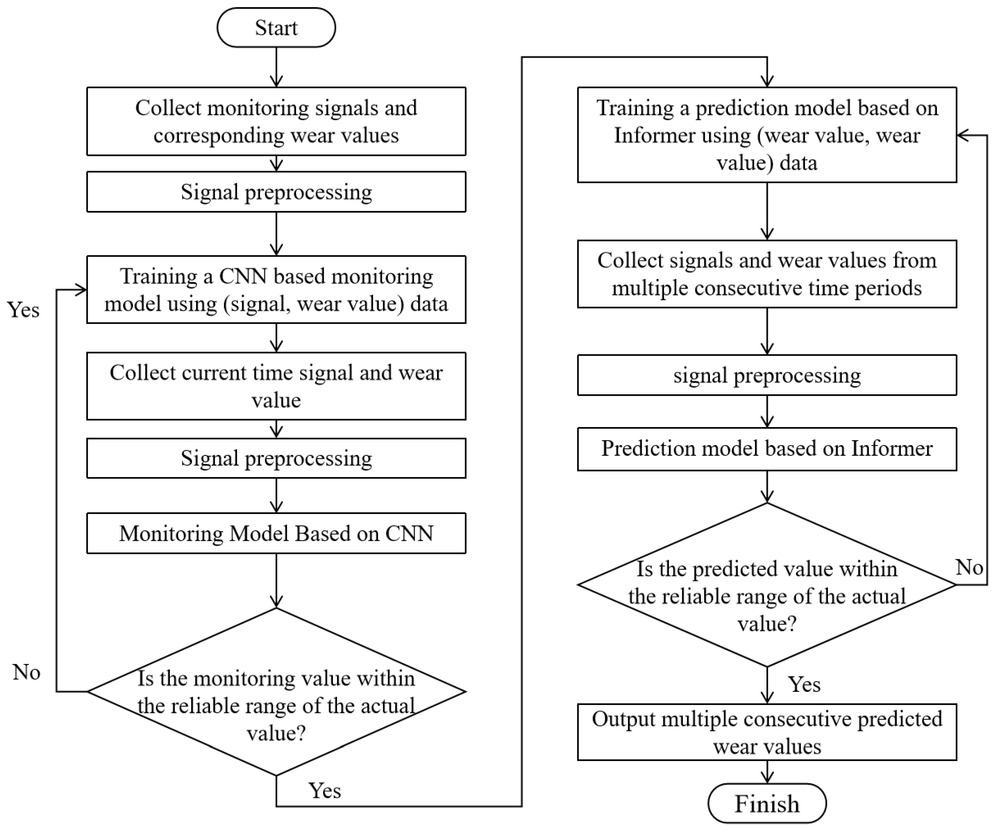
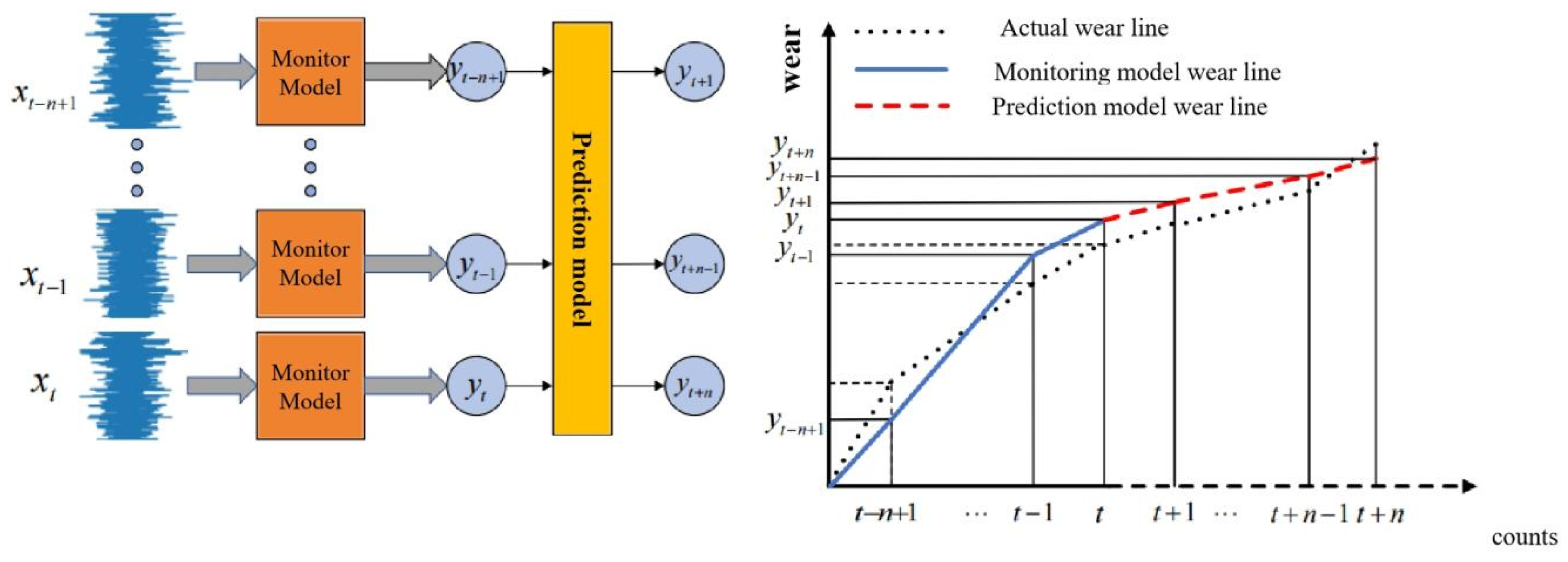
The complete multi-step tool wear prediction framework is illustrated in Figure 3.13. First, during high-speed milling, we collect machine tool status signals via high-precision sensors, including vibration, cutting force, and acoustic emission signals. Simultaneously, we measure the tool’s wear value for each signal, forming a dataset with inputs and corresponding wear values, serving as the basis for future monitoring and prediction models.

Next, the collected signals are input into our pre-established and optimized tool wear monitoring model, based on machine learning or advanced modeling techniques. After training, the model accurately correlates signals with wear values, outputting the current wear value upon input. By continuously inputting signals, we obtain wear values at multiple consecutive time points, reflecting wear changes throughout the machining process.

Finally, these continuous wear values are considered historical data and input into an optimized prediction model, trained to predict future wear based on historical data. This method allows obtaining future wear values at multiple consecutive time points, enabling early prediction of tool wear status.

Figure 3.13. Multi-step Prediction Framework For Tool Wear.

Figure 3.13. Multi-step Prediction Framework For Tool Wear.

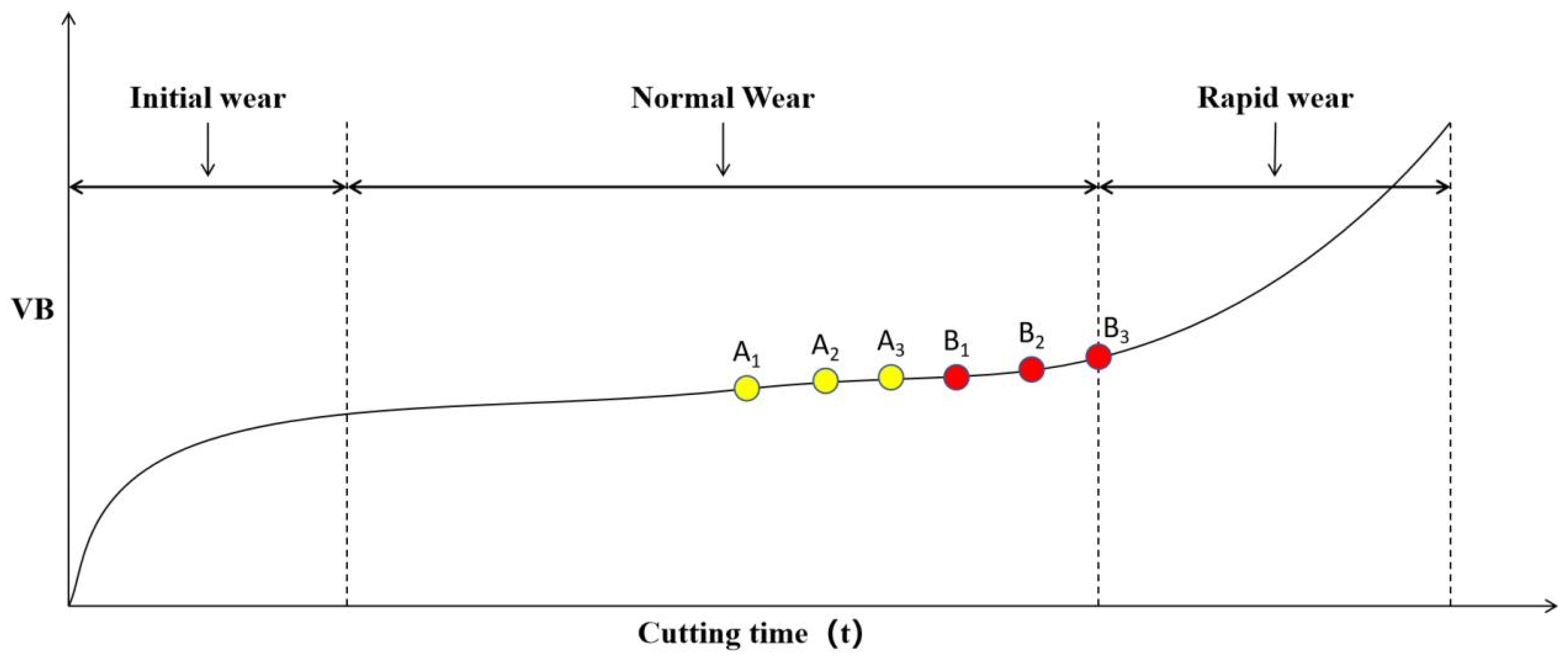
However, in the actual machining process, the machining conditions and tool states at two similar time points will be closer. As shown in Figure 3.14, the tool processing states of A3 and B1 are closer than those of A1 and B1, indicating that the influence of A3 on B1 should be greater than that of A1 on B1. Therefore, continuous multi segment sensor signals are used to monitor the current tool wear values as historical data, namely A1, A2, and A3, and then these historical data are used to predict the tool wear values for a future period of time, namely B1, B2, and B3. The impact of this historical data on the predicted data is different. To address this issue in the future, this chapter introduces the Attention mechanism to assign different weights to different historical input data.

Figure 3.14. Tool wear curve.

Figure 3.14. Tool wear curve.

3.3. Multi Step Prediction Comprehensive Model for Tool Wear

To achieve multi-step advanced prediction of tool wear while accounting for the varying influence of input at different times, we propose a comprehensive model based on the framework above. As shown in Figure 3.15, a tool wear monitoring model using Informer is established to correlate seven signals with wear values via the Informer network, enabling real-time wear monitoring. By inputting consecutive sensor signals, continuous historical wear data is obtained, referring to past wear values. These past wear values are then used to predict future wear.

An Encoder-Decoder framework with the Attention mechanism is adopted for the prediction model, using CNN as a feature extractor to enhance prediction accuracy. The Attention mechanism assigns varying weights to different time inputs, considering the non-uniform impact of past time points on future predictions, aiding in uncovering temporal data dependencies. The comprehensive model can be summarized as:

$$\left\{\begin{array}{c}{(y}_{t+1},y_{t+2},...,y_{t+n})=G(y_{t-n+1},y_{t-n+2},...,y_t)\\ y_t=H\left(X_t\right)=H(x_{t1},x_{t2},x_{t3},x_{t4},x_{t5},x_{t6},x_{t7})\end{array}\right.$$

(3.16)

In the formula, xti - the i-th signal input at time t, i=1, 2, 3, 4, 5, 6, 7;

Xt - Seven signal inputs at time t;

Yt - wear value at time t;

H - Monitoring model computation;

G - Prediction model operation.

Figure 3. 15. Schematic Diagram of Multi-step Prediction Comprehensive Model for Tool Wear.

Figure 3. 15. Schematic Diagram of Multi-step Prediction Comprehensive Model for Tool Wear.

3.3.1. Monitoring Model Based on Informer

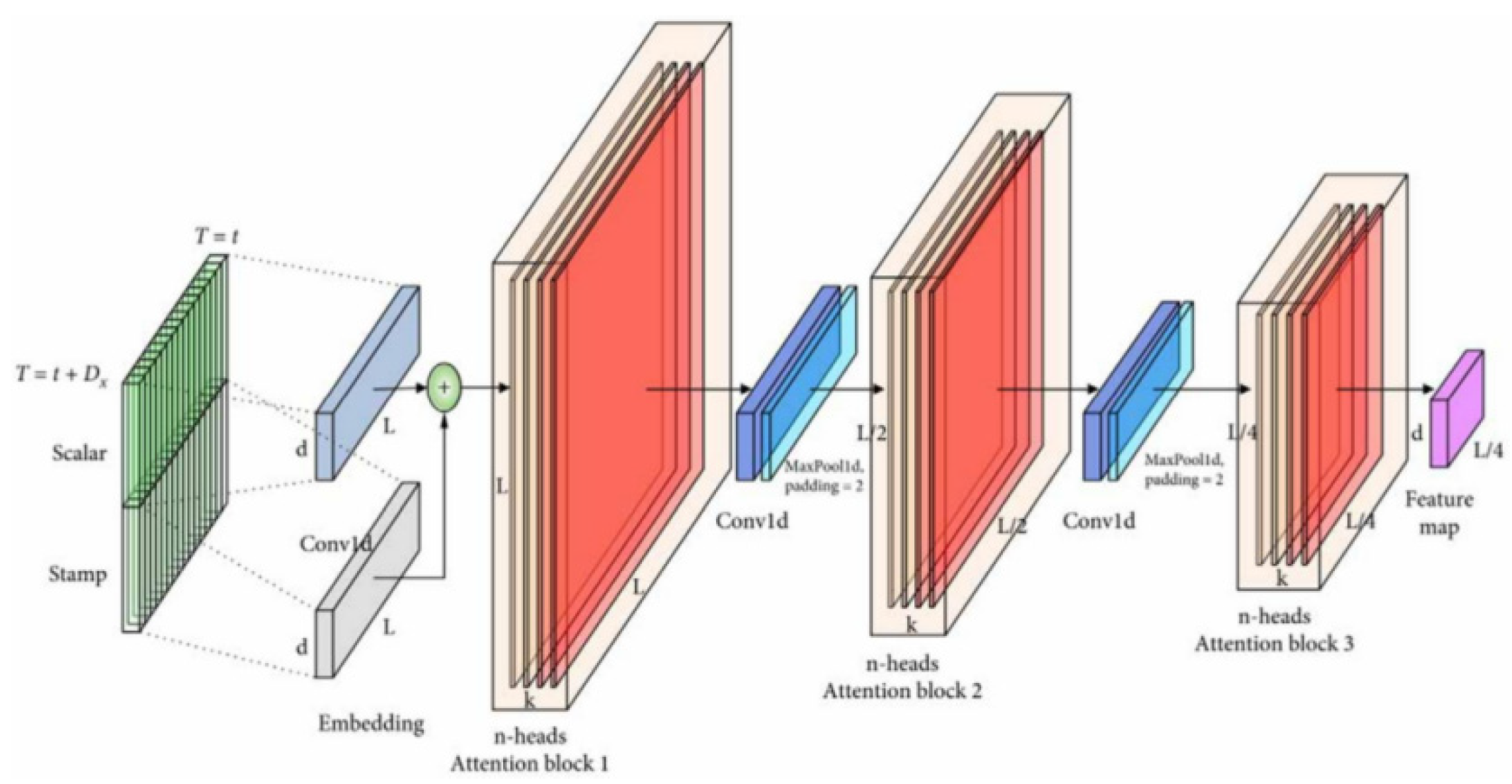
The monitoring model based on Informer is shown in Figure 3.16. The input is a seven dimensional time series signal segment consisting of three-axis force signals, three-axis vibration signals, and acoustic emission signals, and the output is the wear value VB corresponding to the current signal segment.

Figure 3.16. Monitoring Model Based on Informer.

Figure 3.16. Monitoring Model Based on Informer.

By monitoring the model, the tool wear value corresponding to the current signal segment can be obtained. Monitor the wear values of multiple past signal segments and use them as inputs for a predictive model to predict future tool wear values. As shown in Figure 3.17, the prediction model adopts the sequence to sequence structure in NLP, which connects the encoder and decoder with long and short-term information vectors with attention mechanism. The encoder and decoder both use the same GRU subunit, and each intermediate vector contains varying degrees of long and short-term information, depending on the weight assigned by the Attention mechanism. This mechanism can be represented by the following formula:

$$\left\{\begin{array}{c}{c}_j={\displaystyle \sum _{i=1}^n}{a}_{ij}{h}_i\\ a_{ij}={\displaystyle \frac{exp\left(e_{ij}\right)}{\sum _{k=1}^{n}exp\left(e_{kj}\right)}}\\ e_{ij}=score(h_i,s_{j-1})\end{array}\right.$$

(3.17)

In the formula, hi represents the i-th hidden layer of the encoder;

Sj - the jth hidden layer of the decoder;

Eij - the similarity between vectors hi and sj-1, represented by Euclidean distance;

Aij - the weight of the i-th hidden layer in the encoder;

Cj - the jth hidden layer between the encoder and decoder.

Figure 3.17. Encoder Decoder Prediction Model Based on Attention Mechanism.

Figure 3.17. Encoder Decoder Prediction Model Based on Attention Mechanism.

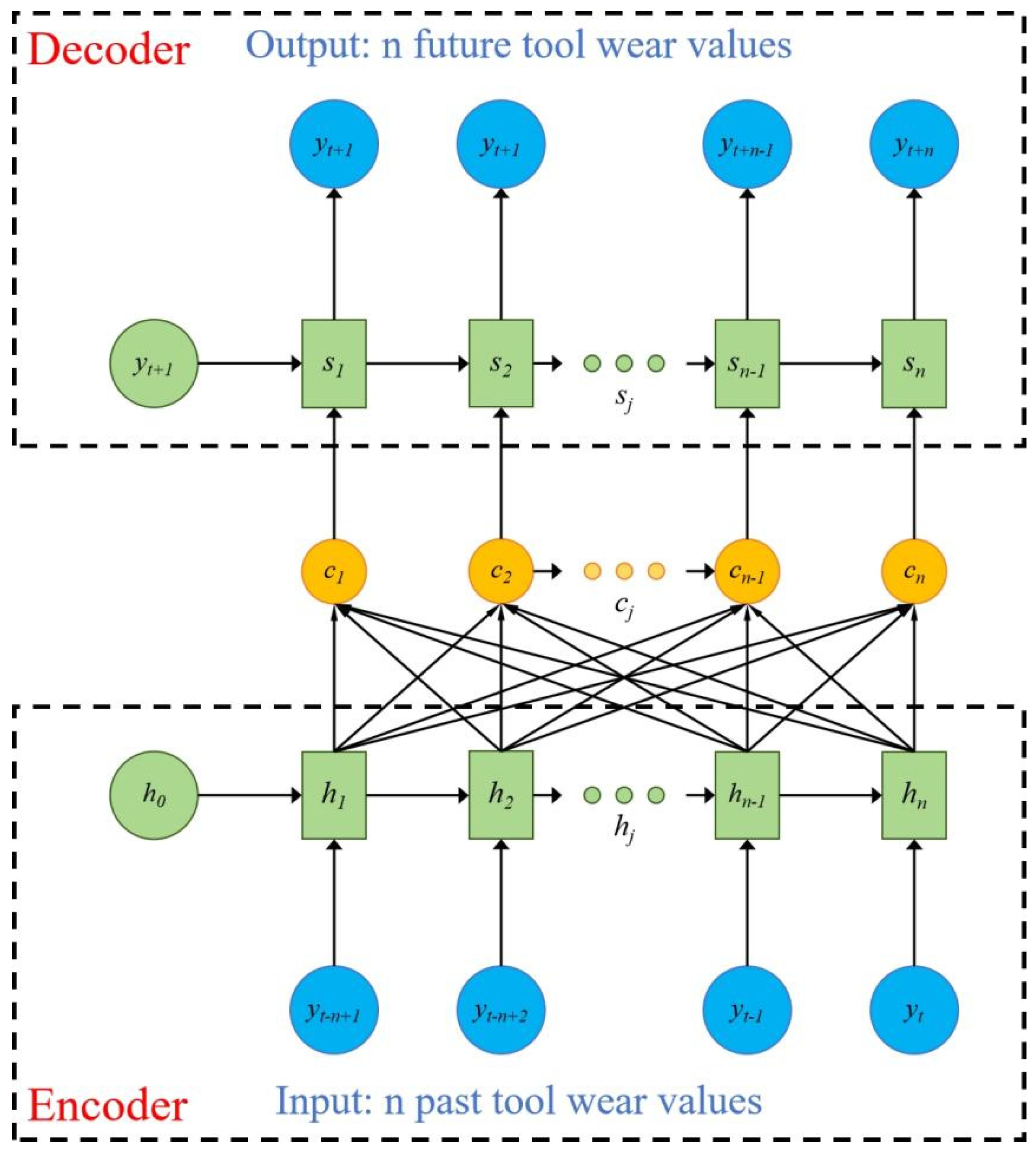
Take multiple consecutive VB values measured recently in the past as inputs to the encoder module, represented by ${\mathrm{y}}_{t-n+1},y_{t-n+2},\dots ,y_t$.N represents the number of input data, which is the number of prediction steps. In the decoder module, n consecutive predicted future VB values will be output,represented by x${\mathrm{y}}_{t+1},y_{t+2},\dots ,y_{t+n}$.Therefore, the model can be represented as:

$$(y_{t+1},y_{t+2},\dots ,y_{t+n})=G(y_{t-n+1},y_{t-n+2},\dots ,y_t)$$

(3.18)

In the formula, y_t represents the wear value at time t;G - Prediction model operation.

3.4. Model Experiment and Result Analysis

3.4.1. Data Settings

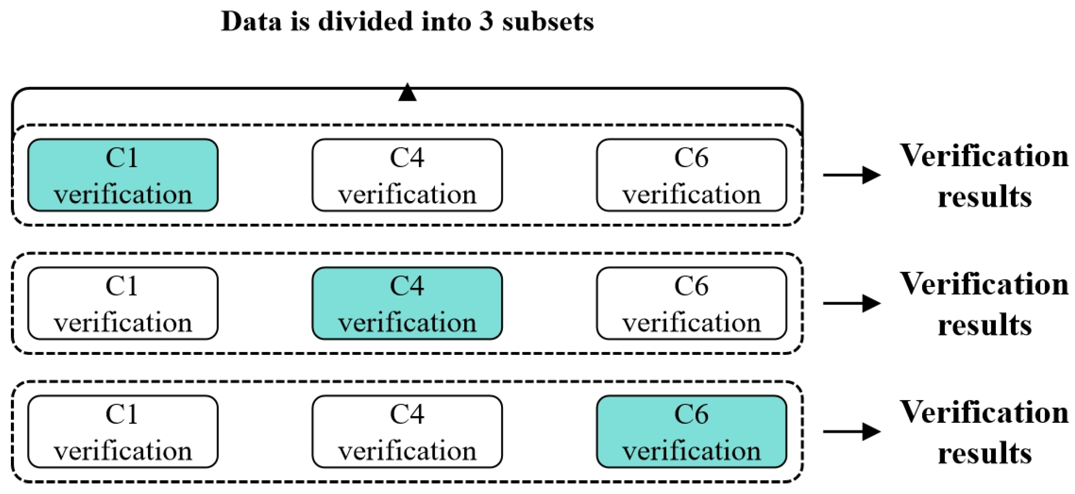
The preprocessed single condition PHM2010 dataset was subjected to three fold cross validation according to C1, C4, and C6, as shown in Figure 3.18. The maximum value of tool wear in three directions was used as a label for model training. The model was updated with weights and bias parameters using a backpropagation algorithm based on the chain rule to minimize the loss function. To validate the predictive performance of the model, the validation set data is input into the trained model to obtain the prediction results of tool wear.

Figure 3.18. Cross Validation.

Figure 3.18. Cross Validation.

3.4.2. Evaluation Criteria

In order to more accurately represent the fitting effect of the model on tool wear monitoring values and real values, and verify the accuracy of the prediction model, based on the regression algorithm evaluation system, this paper objectively evaluates the experimental results using four evaluation indicators, namely mean square error (MSE), root mean square error (RMSE), R-squared value (R-squared), and mean absolute error (MAE). The above evaluation indicators are widely used in regression problems. For the prediction task of tool wear in this article, the formula for evaluation indicators is as follows:

$$MSE={\displaystyle \frac{1}{n}}{\displaystyle \sum _{i=1}^n{(y_i-{\widehat{y}}_i)}^2}$$

(3.19)

$$RMSE=\sqrt{MSE}=\sqrt{{\displaystyle \frac{1}{n}}{\displaystyle \sum _{i=1}^n{(y_i-{\widehat{y}}_i)}^2}}$$

(3.20)

$$R^2=1-{\displaystyle \frac{{\displaystyle \sum _{i=1}^n{(y_i-{\widehat{y}}_i)}^2}}{{\displaystyle \sum _{i=1}^n{(y_i-\overline{y})}^2}}}$$

(3.21)

$$MAE={\displaystyle \frac{1}{n}}{\displaystyle \sum _{i=1}^n\left|y_i-{\widehat{y}}_i\right|}$$

(3.22)

Among them, N represents the number of samples, i represents the sample number,${ \mathrm{y} ^}_{\mathrm{i}}$ represents the i-th tool wear prediction value,$\mathrm{y} ¯$ is the average of the actual values,${\mathrm{y}}_{\mathrm{i}}$ represents the actual value of tool wear for the i-th tool.The ranges of root mean square error (RMSE) and mean absolute error (MAE) are both greater than or equal to zero. When the monitored tool wear value matches the actual tool wear value completely, both RMSE and MAE are zero; When the RMSE and MAE values are higher, it indicates that the model’s prediction accuracy is lower and cannot effectively predict tool wear values.

3.4.3. Experimental Setup

This chapter conducts experiments on the Windows 11 operating system, using PyTorch 2.3.1 and Python 3.9 to build a network and conduct experiments. The experimental hardware platform includes AMD Ryzen 7 6800H@3.20 A GHz CPU with a running memory of 32 GB and an NVIDIA RTX3060 acceleration graphics card with a graphics memory size of 12 GB. The specific experimental configuration is shown in Table 3.1.

Table 3.1. The experimental environment.

Software and Hardware	Name	Notes
CPU	AMD Ryzen 7 6800H	6 cores and 12 threads
GPU	NVIDIA RTX3060	12GB video memory
operating system	Windows	11th generation
development language	Python	3.9.1
development platform	Pycharm	2021.3.2
Deep Learning Framework	Pytorch	2.3.1
GPU acceleration component	CUDA Toolkit	11.8

Table 3.1. The experimental environment.

Software and Hardware	Name	Notes
CPU	AMD Ryzen 7 6800H	6 cores and 12 threads
GPU	NVIDIA RTX3060	12GB video memory
operating system	Windows	11th generation
development language	Python	3.9.1
development platform	Pycharm	2021.3.2
Deep Learning Framework	Pytorch	2.3.1
GPU acceleration component	CUDA Toolkit	11.8

To enhance model performance and suppress overfitting, a batch strategy is employed for training, expediting the process and improving generalization. Adam optimizer with a step decay strategy for learning rate reduction, coupled with Dropout regularization and early stopping, further prevents overfitting. Hyperparameters are selected via grid search on the validation set, with the optimal combination shown in Table 3.2. This configuration is consistent across comparison and ablation experiments for reliability.

Table 3.2. Hyperparameter setting.

Hyper-Parameters	Describe	Numerical/Method
Epoch	Training epochs	500
Batch size	batch size	30
Learning rate	Learning rate	0.001
Gamma	Learning rate adjustment multiplier	0.5
Step size	The number of intervals between a decrease in learning rate	50
Activation Function	activation function	ReLU
Dropout	Discard rate	0.3

Table 3.2. Hyperparameter setting.

Hyper-Parameters	Describe	Numerical/Method
Epoch	Training epochs	500
Batch size	batch size	30
Learning rate	Learning rate	0.001
Gamma	Learning rate adjustment multiplier	0.5
Step size	The number of intervals between a decrease in learning rate	50
Activation Function	activation function	ReLU
Dropout	Discard rate	0.3

3.4.4. Model Parameter Determination Experiment

This chapter explores the effects of downsampling on sensor data integrity and how model parameters shape experimental outcomes. Using C1 and C6 as training sets and C4 as the validation set, we assess various factors’ impacts. By analyzing different downsampled time series lengths, we evaluate data loss’s effect on model performance. Table 3.3 shows the results: shorter downsampling lengths lead to significant data loss and model errors during training and testing. To balance information integrity and computational efficiency, we chose 5000 data points as the downsampled length. This approach minimizes information loss, maintains high training and validation accuracy, reduces computational load, prevents overfitting, and enhances the model’s generalization to new data.

Table 3.3. Comparison of length results after downsampling.

Length of Time Series Data After Downsampling	MSE	RMSE	R2	MAE
100	1,184.942	34.423	0.874	29.687
500	658.230	25.656	0.882	18.334
1000	358.913	18.945	0.896	14.878
2000	264.160	16.253	0.901	10.694
3000	249.293	15.789	0.940	8.687
4000	68.310	8.265	0.976	5.768
5000	5.890	2.427	0.993	2.362
6000	13.323	3.650	0.983	2.679

Table 3.3. Comparison of length results after downsampling.

Length of Time Series Data After Downsampling	MSE	RMSE	R2	MAE
100	1,184.942	34.423	0.874	29.687
500	658.230	25.656	0.882	18.334
1000	358.913	18.945	0.896	14.878
2000	264.160	16.253	0.901	10.694
3000	249.293	15.789	0.940	8.687
4000	68.310	8.265	0.976	5.768
5000	5.890	2.427	0.993	2.362
6000	13.323	3.650	0.983	2.679

To determine optimal tool wear prediction model parameters, experiments were conducted to confirm neural network layer sizes, including convolutional layer sizes and the sampling factor of the probabilistic sparse self-attention mechanism. In convolutional neural networks, convolution kernel size impacts feature capture range; inappropriate sizes lead to inaccurate feature extraction. Probabilistic sparse self-attention reduces complexity while maintaining performance; sampling factor selection affects long-range dependency capture and efficiency. Table 3.4 illustrates convolution kernel size effects on prediction results, using MSE, RMSE, R-squared, and MAE for evaluation.

Table 3.4. Effect of convolution kernel size on experimental results.

Convolutional kernel size	MSE	RMSE	R2	MAE
1	13.609	3.689	0.891	5.014
2	10.081	3.175	0.928	4.785
3	8.738	2.956	0.956	4.598
4	4.951	2.225	0.994	3.254
5	22.043	4.695	0.986	5.201
6	18.931	4.351	0.975	5.469
7	17.986	4.241	0.981	5.954

Table 3.4. Effect of convolution kernel size on experimental results.

Convolutional kernel size	MSE	RMSE	R2	MAE
1	13.609	3.689	0.891	5.014
2	10.081	3.175	0.928	4.785
3	8.738	2.956	0.956	4.598
4	4.951	2.225	0.994	3.254
5	22.043	4.695	0.986	5.201
6	18.931	4.351	0.975	5.469
7	17.986	4.241	0.981	5.954

The experimental results indicate that a convolution kernel size of 4 yields the best prediction performance, enabling better local feature capture. Hence, a kernel size of 4 is used in subsequent experiments.

The sampling factor c in probabilistic sparse self-attention significantly impacts model performance. Table 3.5 shows that c=15 offers optimal performance, as it balances the trade-off between computational efficiency and information richness, ensuring efficient sequence data handling.

Table 3.5. Influence of sampling factor c on experimental results.

Sampling Factor Size	MSE	RMSE	R2	MAE	Training time (s)
1	36.978	6.081	0.872	7.974	668
3	33.651	5.801	0.897	7.161	1012
5	27.164	5.212	0.923	6.091	1237
7	21.836	4.673	0.931	5.922	1453
9	12.996	3.605	0.955	5.687	1503
11	6.325	2.515	0.971	4.230	1613
13	5.579	2.362	0.989	3.986	1527
15	4.674	2.162	0.991	3.636	2129
17	9.960	3.156	0.990	4.579	2263
19	10.634	3.261	0.975	4.307	2372
21	20.277	4.503	0.971	6.079	2656

Table 3.5. Influence of sampling factor c on experimental results.

Sampling Factor Size	MSE	RMSE	R2	MAE	Training time (s)
1	36.978	6.081	0.872	7.974	668
3	33.651	5.801	0.897	7.161	1012
5	27.164	5.212	0.923	6.091	1237
7	21.836	4.673	0.931	5.922	1453
9	12.996	3.605	0.955	5.687	1503
11	6.325	2.515	0.971	4.230	1613
13	5.579	2.362	0.989	3.986	1527
15	4.674	2.162	0.991	3.636	2129
17	9.960	3.156	0.990	4.579	2263
19	10.634	3.261	0.975	4.307	2372
21	20.277	4.503	0.971	6.079	2656

After determining the optimal network parameter model, the relevant hyperparameters of each layer for the CNN Informer neural network model proposed in this chapter are shown in Table 3.6.

Table 3.6. Neural network model hyperparameters.

Network Layer	Parameter	Output Matrix Dimension
Input	-	(5000, 7)
Convolutional Layer	Kernel=4, Stride=4, output channel=128	(1250, 128)
Maximum pooling layer	Kernel=3, Stride=2	(624, 128)
Probabilistic Sparse Self Attention Mechanism 1	Head number=8, c=15	(624, 128)
Distillation layer 1	Conv1d: Kernel=3, Stride=2, channel=128 Maxpooling: Kernel=3, Stride=2	(155, 128)
Probabilistic Sparse Self Attention Mechanism 2	Head number=8, c=15	(155, 128)
Distillation layer 2	Conv1d: Kernel=3, Stride=2, channel=72 Maxpooling:Kernel=3, Stride=2	(38, 72)
Probability Sparse Self Attention Mechanism 3	Head number=8, c=15	(38, 72)
Distillation layer 3	Conv1d: Kernel=3, Stride=1, channel=64 Maxpooling: Kernel=3, Stride=2	(18, 64)
Fully connected layer	Output dim = 64	(1, 64)
Fully connected layer	Output dim = 16	(1, 16)
Fully connected layer	Output dim = 1	(1, 1)

Table 3.6. Neural network model hyperparameters.

Network Layer	Parameter	Output Matrix Dimension
Input	-	(5000, 7)
Convolutional Layer	Kernel=4, Stride=4, output channel=128	(1250, 128)
Maximum pooling layer	Kernel=3, Stride=2	(624, 128)
Probabilistic Sparse Self Attention Mechanism 1	Head number=8, c=15	(624, 128)
Distillation layer 1	Conv1d: Kernel=3, Stride=2, channel=128 Maxpooling: Kernel=3, Stride=2	(155, 128)
Probabilistic Sparse Self Attention Mechanism 2	Head number=8, c=15	(155, 128)
Distillation layer 2	Conv1d: Kernel=3, Stride=2, channel=72 Maxpooling:Kernel=3, Stride=2	(38, 72)
Probability Sparse Self Attention Mechanism 3	Head number=8, c=15	(38, 72)
Distillation layer 3	Conv1d: Kernel=3, Stride=1, channel=64 Maxpooling: Kernel=3, Stride=2	(18, 64)
Fully connected layer	Output dim = 64	(1, 64)
Fully connected layer	Output dim = 16	(1, 16)
Fully connected layer	Output dim = 1	(1, 1)

3.4.5. Experimental Result

In addition to training the results of the network model designed in this paper, the experiment also compared with a series of models such as one-dimensional convolutional neural model and Informer model, which verified that the network of a single module could not predict the tool wear accurately. Therefore, the neural network structure was improved by fusing the advantages of each module to obtain more accurate prediction values. The experimental results of the model proposed in this chapter are shown in the blue, orange, and green curves in Figure 3.14, which represent the tool wear prediction results for C1, C4, and C6, respectively.

Figure 3.19. This paper presents the experimental results of cross-validation of the network model.

Figure 3.19. This paper presents the experimental results of cross-validation of the network model.

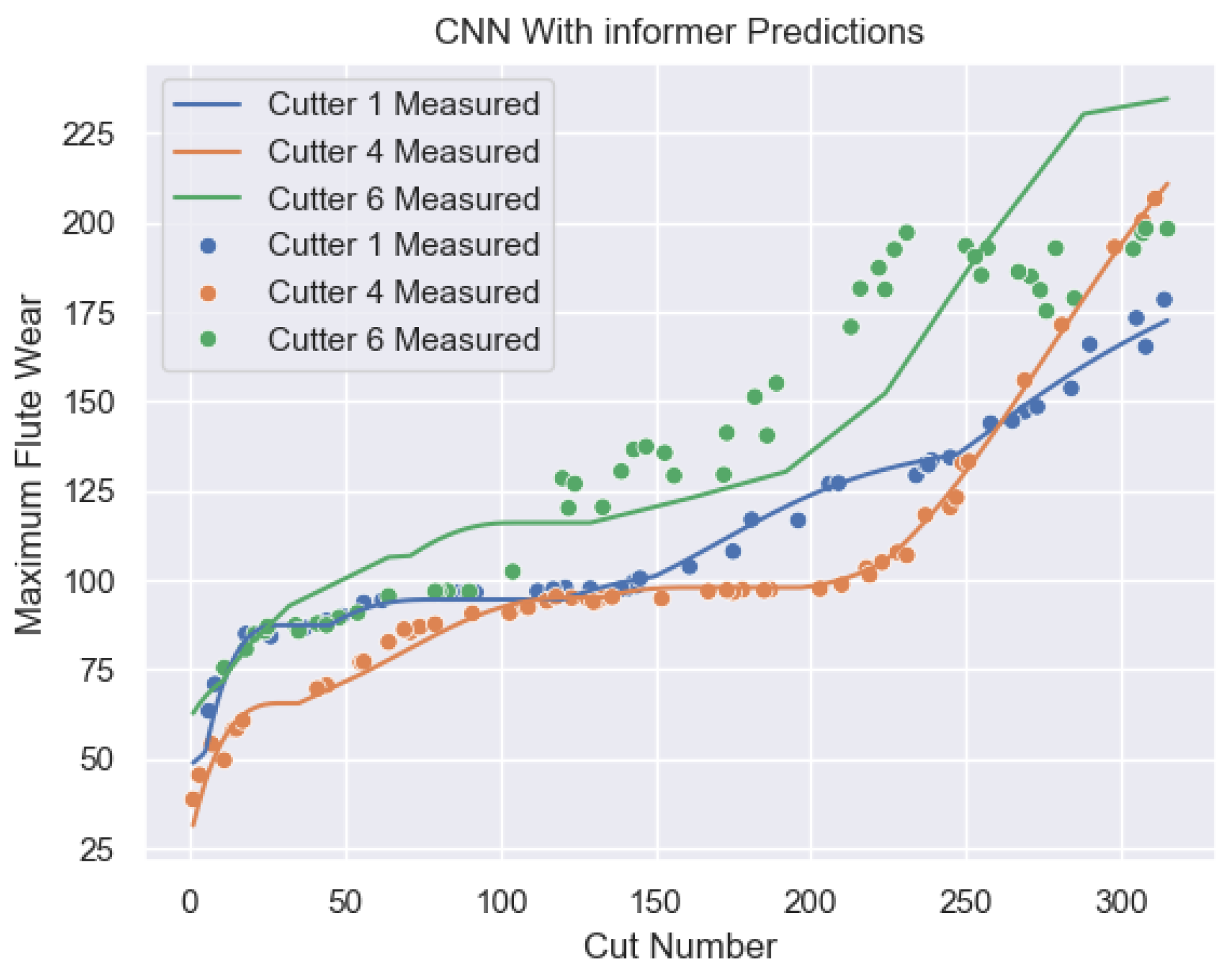
To assess the network’s feature extraction effectiveness, we conducted a feature correlation analysis. We sampled high-dimensional features (dim: 1,64) before the fully connected layer and used Pearson correlation and mutual information to measure their relationship with the maximum tool wear (315 times C1 max). Pearson correlation, ranging from -1 to 1, indicates linear dependence, with higher values suggesting stronger correlation. Mutual information quantifies nonlinear correlations, with larger values indicating stronger dependence. Traditional machine learning sets a Pearson correlation threshold of 0.5 for feature selection. Our analysis (Table 3.9) revealed high Pearson and mutual information values, confirming strong linear and nonlinear correlations between extracted features and max wear.

Specifically, the Pearson correlation coefficients of some features are significantly higher than the threshold of 0.5, and the mutual information values also show significant values, which further confirms the effectiveness of these features. Therefore, these results not only support the effectiveness of network feature extraction, but also provide a strong feature foundation for subsequent model construction. Through this analysis, we can ensure that the features used not only meet traditional correlation standards, but also exhibit excellent performance within the framework of deep networks, providing a reliable basis for practical applications such as tool wear prediction.

Table 3.9. High dimensional feature correlation.

	1st dimensional feature	7th dimensional feature	42nd dimensional feature	60th dimensional feature
Pearson Correlation Coefficient	0.9004	0.9273	0.8995	0.9615
Mutual information	0.8794	0.9864	0.8162	0.9946

Table 3.9. High dimensional feature correlation.

	1st dimensional feature	7th dimensional feature	42nd dimensional feature	60th dimensional feature
Pearson Correlation Coefficient	0.9004	0.9273	0.8995	0.9615
Mutual information	0.8794	0.9864	0.8162	0.9946

And high-dimensional features were reduced using T-SNE method, and the distribution of each sample’s features in three-dimensional space is shown in Figure 3.20. From the figure, it can be seen that the high-dimensional features extracted by the deep fusion neural network are automatically stacked together and distributed in three-dimensional space after dimensionality reduction. In the t-SNE graph, each data point represents a sample in the original high-dimensional space, and its position under the t-SNE mapping represents its position in the low dimensional space. There are natural clusters in the data points, which are presented in a tightly clustered form. Moreover, the data points are denser within the clusters, and the distance between different clusters is relatively far, which is consistent with the early, middle, and severe wear processes of the tool. This further proves that the network structure proposed in this paper can extract features with strong correlation with tool wear.

Figure 3.20. t-SEN high dimensional feature distribution map.

Figure 3.20. t-SEN high dimensional feature distribution map.

3.4.6. Comparative Experiment

To verify the superiority of multi-sensor data fusion (MSDF) technology, this study systematically evaluated the predictive performance of force signal sensors (FS), acceleration sensors (ACC), and acoustic emission sensors (AES) when used independently. The data from each sensor was separately introduced into the prediction model for tool wear detection. Research results (Table 3.8) revealed significant limitations of single sensors in capturing comprehensive tool wear information, leading to substantial deviations from actual wear situations.

Comparative analysis indicates that single sensors offer limited information, unable to cover complex tool wear changes, resulting in inaccurate predictions. Multi-sensor data fusion (MSDF) leverages the strengths of different sensors: force signal sensors track cutting force dynamics, acceleration sensors capture vibration characteristics, and acoustic emission sensors monitor internal stress and crack propagation. Integrating these multi-source data builds a more comprehensive tool wear model, significantly enhancing prediction accuracy and reliability. This validates the efficacy of MSDF in practical applications and provides a theoretical basis and technical pathway for optimizing prediction models and improving tool management efficiency.

Table 3.8. High dimensional feature correlation.

Types of sensors	C1			C4			C6
	MAE	R2	RMSE	MAE	R2	RMSE	MAE	R2	RMSE
Force Signal	6.155	0.953	7.246	7.834	0.934	8.451	7.021	0.955	9.076
acceleration signal	6.795	0.941	8.314	7.596	0.952	9.772	6.750	0.975	8.312
acoustic emission signal	9.312	0.933	10.566	9.432	0.944	10.876	8.324	0.971	9.767
Force and acceleration signals	6.5	0.978	5.109	6.878	0.985	6.918	4.618	0.989	4.221
Force, acceleration, and acoustic emission signals	1.693	0.995	3.628	2.132	0.992	3.627	2.173	0.997	3.159

Table 3.8. High dimensional feature correlation.

Types of sensors	C1			C4			C6
	MAE	R2	RMSE	MAE	R2	RMSE	MAE	R2	RMSE
Force Signal	6.155	0.953	7.246	7.834	0.934	8.451	7.021	0.955	9.076
acceleration signal	6.795	0.941	8.314	7.596	0.952	9.772	6.750	0.975	8.312
acoustic emission signal	9.312	0.933	10.566	9.432	0.944	10.876	8.324	0.971	9.767
Force and acceleration signals	6.5	0.978	5.109	6.878	0.985	6.918	4.618	0.989	4.221
Force, acceleration, and acoustic emission signals	1.693	0.995	3.628	2.132	0.992	3.627	2.173	0.997	3.159

In order to verify that a single network cannot effectively achieve the nonlinear relationship between signal data and wear values, this paper validates the results of three single network models (one-dimensional convolutional neural network model, one-dimensional convolutional neural network attention mechanism model, one-dimensional convolutional neural network Informer model). The one-dimensional convolutional neural network is designed with reference to the Resnet network structure, and the convolution operation is changed to one-dimensional convolution. Other model parameters refer to the convolution module in this article; The parameter settings for the one-dimensional convolutional neural network Attention mechanism model and one-dimensional convolutional neural network Informer model refer to the Informer module parameters used in this article.

The experimental results comparing the predicted and actual tool wear values of the one-dimensional convolutional neural model are shown in Figure 3.21; The experimental results comparing the predicted and actual tool wear values of the one-dimensional convolutional neural network Attention mechanism model are shown in Figure 3.22; The experimental results comparing the predicted and actual tool wear values of the one-dimensional convolutional neural network Informer model are shown in Figure 3.23.

Figure 3.21. Tool wear prediction of one-dimensional convolutional neural network model.

Figure 3.21. Tool wear prediction of one-dimensional convolutional neural network model.

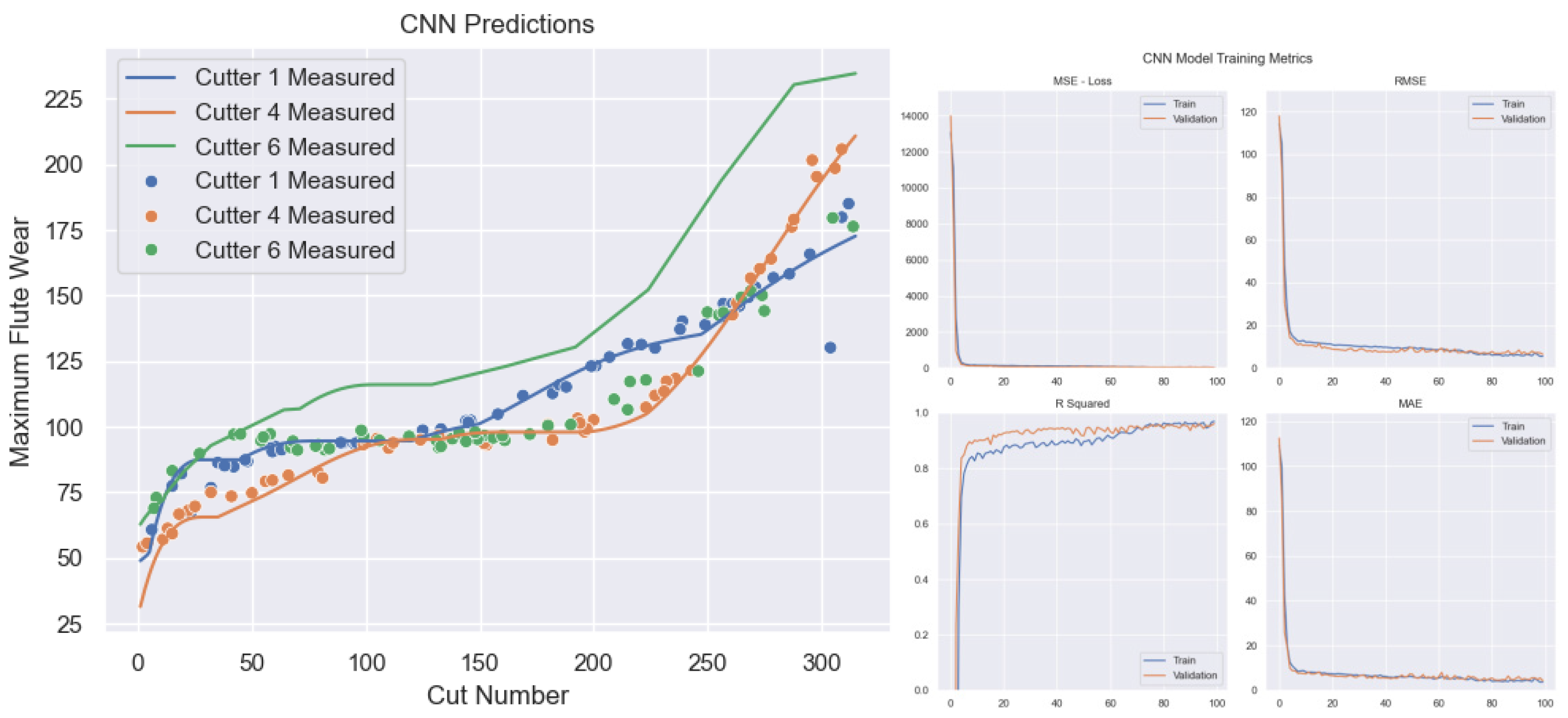
Figure 3.22. One dimensional Convolutional Neural Network Attention Mechanism Model for Predicting Tool Wear.

Figure 3.22. One dimensional Convolutional Neural Network Attention Mechanism Model for Predicting Tool Wear.

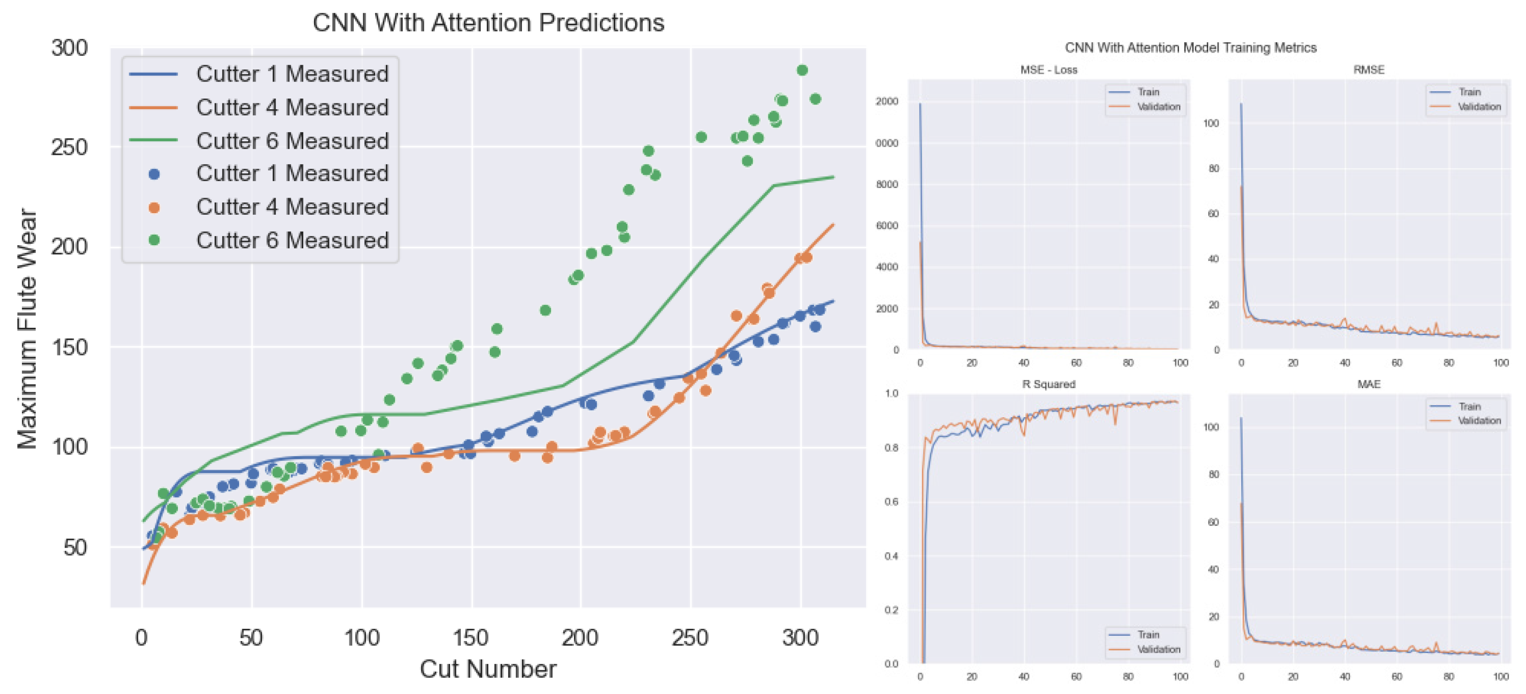
Figure 3.23. One dimensional Convolutional Neural Network - Informer Model for Predicting Tool Wear.

Figure 3.23. One dimensional Convolutional Neural Network - Informer Model for Predicting Tool Wear.

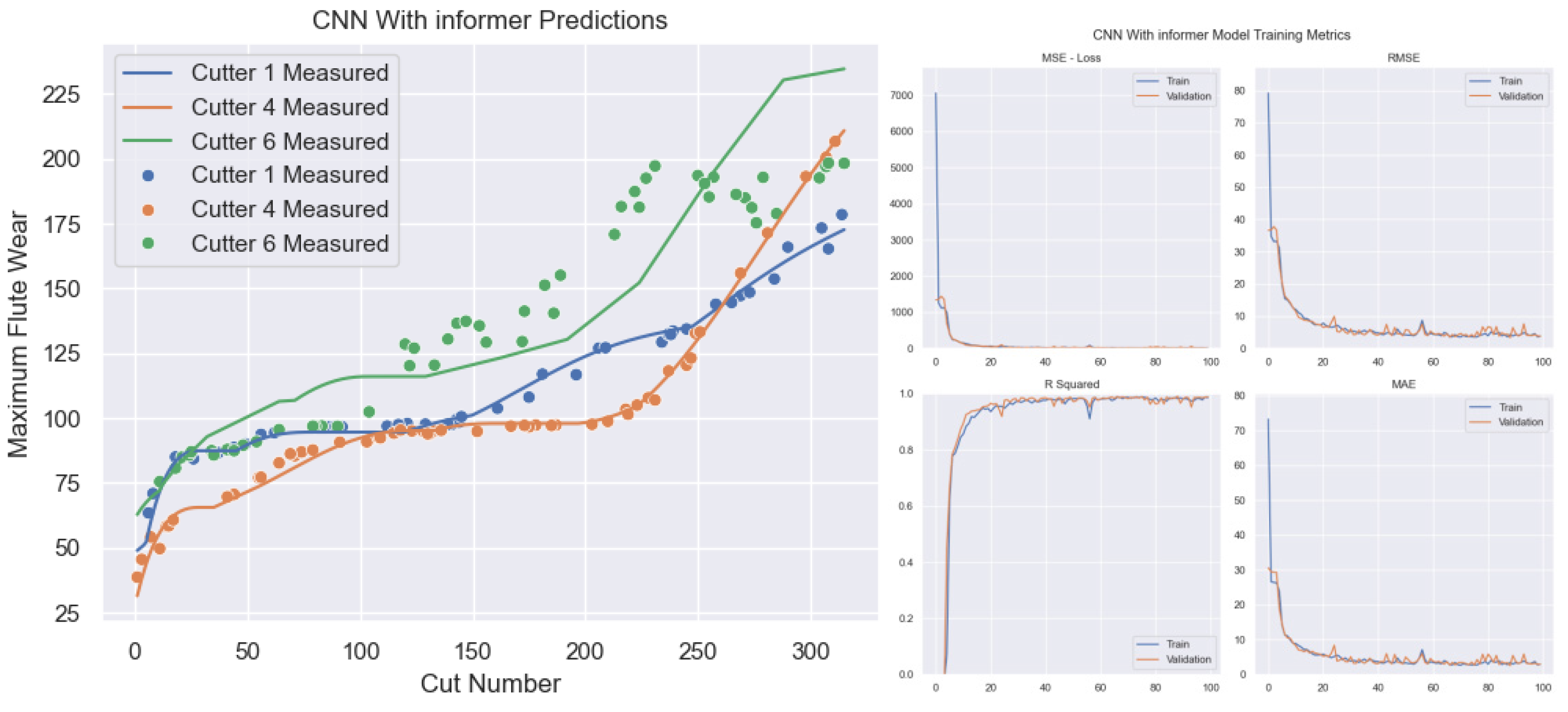
Comparing model performance across different wear stages reveals each model’s limitations. Figure 3.21 shows the 1D CNN has significant errors in initial and severe wear stages, indicating difficulty in capturing rapid wear transitions. Figure 3.22 shows the CNN Attention model has small errors on specific sets (C4, C6) but poor cross-validation performance on others (C1), highlighting its limited generalization. Figure 3.23 shows the CNN Informer model’s predictions closely follow the true curve but has jumps and local deviations, making it challenging to perfectly simulate dynamic wear processes.

A single network model struggles to comprehensively extract key features from long-term sensor data. This study proposes a fusion model strategy to leverage different models’ strengths for more comprehensive data interpretation and accurate signal-to-wear mapping. Comparative experiments (Table 3.9) show the proposed model outperforms others in evaluation metrics, effectively learning wear curve patterns.

Table 3.11. Comparison of experimental results under different methods.

Model name	C1			C4			C6
	MAE	R2	RMSE	MAE	R2	RMSE	MAE	R2	RMSE
SVR [38]	1.56	0.871	18.5	-	0.882	-	24.9	0.892	31.5
LSTM [63]	24.5	0.863	31.2	18	0.923	20	24.8	0.845	31.4
CNN [64]	6.57	0.928	9.46	15.75	0.918	20.63	17.68	0.899	22.34
CNN-LSTM [65]	8.3	0.936	12.1	-	0.922	-	15.2	0.917	18.9
TBNN [38]	11.18	0.897	13.77	9.39	0.954	11.85	11.34	0.936	14.33
CTNN [39]	4.294	0.976	6.116	-	0.941	-	7.772	0.936	9.553
IE-SBIGRU [40]	3.634	0.966	5.358	-	0.959	-	7.753	0.964	9.209
Our	1.693	0.995	3.628	2.132	0.992	3.627	2.173	0.997	3.159

Table 3.11. Comparison of experimental results under different methods.

Model name	C1			C4			C6
	MAE	R2	RMSE	MAE	R2	RMSE	MAE	R2	RMSE
SVR [38]	1.56	0.871	18.5	-	0.882	-	24.9	0.892	31.5
LSTM [63]	24.5	0.863	31.2	18	0.923	20	24.8	0.845	31.4
CNN [64]	6.57	0.928	9.46	15.75	0.918	20.63	17.68	0.899	22.34
CNN-LSTM [65]	8.3	0.936	12.1	-	0.922	-	15.2	0.917	18.9
TBNN [38]	11.18	0.897	13.77	9.39	0.954	11.85	11.34	0.936	14.33
CTNN [39]	4.294	0.976	6.116	-	0.941	-	7.772	0.936	9.553
IE-SBIGRU [40]	3.634	0.966	5.358	-	0.959	-	7.753	0.964	9.209
Our	1.693	0.995	3.628	2.132	0.992	3.627	2.173	0.997	3.159

References

- Ding Yufa Research on Online Tool Wear Identification Technology for Mass Production [D] Wuhan: Master’s thesis from Huazhong University of Science and Technology, 2011: 8-9.
- Kurada S, Bradley C. A Review of Machine Vision Sensors for Tool Condition Monitoring[J]. Computers in Industry, 1997, 34: 55-72.
- Tsai, M.-H.; Chen, T.-H.; Lee, J.-N.; Hsu, T.-L.; Huang, D.-K. Five-Axis Finish Milling Machining for an Inconel 718 Alloy Monolithic Blisk. Appl. Sci. 2024, 14, 4015. [Google Scholar] [CrossRef]
- Javed K, Gouriveau R, Li X, et al. Tool wear monitoring and prognostics challenges: a comparison of connectionist methods toward an adaptive ensemble model[J]. Journal of Intelligent Manufacturing, 2018, 29: 1873-1890.
- Zhou Chengpeng,Tool wear prediction method based on deep learning [D] Shenzhen: University of the Chinese Academy of Sciences, 2022.
- Li Y, Liu C, Hua J, et al. A novel method for accurately monitoring and predicting tool wear under varying cutting conditions based on meta-learning[J]. CIRP Annals, 2019, 68(1): 487-490.
- Gdula, M.; Knapčíková, L.; Husár, J.; Vandžura, R. Modeling and Measurement of Tool Wear During Angular Positioning of a Round Cutting Insert of a Toroidal Milling Tool for Multi-Axis Milling. Appl. Sci. 2024, 14, 10405. [Google Scholar] [CrossRef]
- Dan L, Mathew J. Tool Wear and Failure Monitoring Techniques for Turning—A Review[J]. International Journal of Machine Tools and Manufacture, 1990, 30(4): 579-598.
- Zhang Kaifeng,Research on Tool Wear Monitoring Method Based on Multi Sensor Information Fusion [D] Shenyang: Doctoral Dissertation of Northeastern University, 2016: 14-15.
- Zhang C, Zhang J. On-line Tool Wear Measurement for Ball-end Milling Cutter Based on Machine Vision[J]. Computers in Industry, 2013, 64(6): 708-719.
- Guan Shengqi, Chen Yongdang, Ren Lang, etc Tool wear detection driven by visual target features [J] Journal of Xi’an Engineering University, 2018, 32 (4): 474-478.
- Chawla R, Bhattacharya S L. Multispeed Tool-life Tests with Radioactive Tools[J]. Wear, 1978, 46(2):309-319.
- Liu Bin, Ren Yuyan, Feng Jining Research on Monitoring Methods for CNC Lathe Tools [J] Mechanical Research and Application, 2003, 16 (2): 44-45.
- Zhu K, Zhang Y. A Generic Tool Wear Model and its Application to Force Modeling and Wear Monitoring in High Speed Milling[J]. Mechanical Systems and Signal Processing, 2019, 115: 147-161.
- Rmili W, Ouahabi A, Serra R, et al. An Automatic System Based on Vibratory Analysis for Cutting Tool Wear Monitoring[J]. Measurement, 2016, 77: 117-123.
- Ren Q, Balazinski M, Baron L, et al. Type-2 Fuzzy Tool Condition Monitoring System Based on Acoustic Emission in Micro-milling[J]. Information Sciences, 2014, 255: 121-134.
- Elgargni M A, Al-Habaibeh A. Analytical and Comparative Study of using A CNC Machine Spindle Motor Power and Infrared Technology for the Design of a Cutting Tool Condition Monitoring System[C]. Cambridge, UK: INDIN, 2015: 782-787.
- Liu Tongshun,Monitoring and process optimization of micro milling tool wear based on hidden Markov model [D] Hefei: Doctoral Dissertation of University of Science and Technology of China, 2018: 21-22.
- Zhao, P.; Song, Y.; Jiang, B.; Wang, B. Distribution and Prediction of Incremental Cutter Flank Wear in High-Efficiency Milling. Appl. Sci. 2023, 13, 4749. [Google Scholar] [CrossRef]
- Xie Yangyang,Research on Tool State Recognition Based on Acoustic Emission and Deep Learning [D] Nanjing: Master’s thesis from Nanjing University of Information Science and Technology, 2017: 11-14.
- Yang Yong,Vibration monitoring method for tool wear of CNC machine tools [J] Mechanical, 2009, 36 (7): 58-60.
- Wang Peixin Research on the Wear Monitoring System of Turning Tools [D] Kunming: Master’s thesis of Kunming University of Science and Technology, 2018:6-7.
- Li Bin, Ding Yufa, Liu Hongqi Application of Wavelet Packet Analysis Technology in Current Tool Wear Monitoring System [J] Mind and Computation, 2010 (4): 258-264.
- Harun M, Ghazali M F, Yusoff A R. Tri-axial Time-frequency Analysis for Tool Failures Detection in Deep Twist Drilling Process[J]. Procedia CIRP, 2016, 46: 508-511.
- Kumar H S, Pai P S, Sriram N S, et al. Selection of Mother Wavelet for Effective Wavelet Transform of Bearing Vibration Signals[J]. Advanced Materials Research, 2014, 1039: 169-176.
- Yoon M C, Chin D H. Cutting Force Monitoring in the Endmilling Operation for Chatter Detection[J]. Proceeding of the Institute of Mechanical Engineers.part B.journal of Engineering Manufacture, 2005, 219(6): 455-465.
- Drouillet C, Karandikar J, Nath C, et al. Tool Life Predictions in Milling using Spindle Power with the Neural Network Technique[J]. Journal of Manufacturing Processes, 2016, 22: 161-168.
- Wiciak-Pikua M, Felusiak-Czyryca A, Twardowski P. Tool Wear Prediction Based on Artificial Neural Network during Aluminum Matrix Composite Milling[J]. Sensors, 2020, 20(20): 5798.
- Feito N, Muoz-Sánchez A, Díaz-Lvarez A, et al. Analysis of the Machinability of Carbon Fiber Composite Materials in Function of Tool Wear and Cutting Parameters Using the Artificial Neural Network Approach[J]. Materials, 2019, 12(17): 2747.
- Cheng Can, Li Jianyong, Xu Wensheng, etc Tool wear state recognition based on support vector machine and particle filter [J] Vibration and Shock, 2018, 37 (17): 56-63.
- Albina, Jegorowa, Jarosaw, et al. Initial Study on the Use of Support Vector Machine (SVM) in Tool Condition Monitoring in Chipboard Drilling[J]. European Journal of Wood and Wood Products, 2019, 77(5): 957-959.
- Pandiyan V, Caesarendra W, Tjahjowidodo T, et al. In-process Tool Condition Monitoring in Compliant Abrasive Belt Grinding Process Using Support Vector Machine and Genetic Algorithm[J]. Journal of Manufacturing Processes, 2018, 31: 199-213.
- Lv Junjie, Wang Jie, Wang Mei Research on Tool Wear Monitoring Based on SOM and HMM Combination [J] China Mechanical Engineering, 2010, 21 (13): 1531-1535.
- Zhang C, Yao X, Zhang J, et al. Tool Wear Monitoring Based on Deep Learning[J]. Computer Integrated Manufacturing Systems, 2017, 23(10): 2146-2155.
- Kothuru A, Nooka S P, Liu R. Application of Deep Visualization in CNN-based Tool Condition Monitoring for End Milling[J]. Procedia Manufacturing, 2019, 34: 995-1004.
- Wu, L.; Sha, K.; Tao, Y.; Ju, B.; Chen, Y. A Hybrid Deep Learning Model as the Digital Twin of Ultra-Precision Diamond Cutting for In-Process Prediction of Cutting-Tool Wear. Appl. Sci. 2023, 13, 6675. [Google Scholar] [CrossRef]
- Tang K, Wang X, Hu W, et al. Research on Tool Wear Prediction Based on Deep Residual Network[C]. Jinan, China: IWMECS, 2018: 325-329.
- Li, Z.; Zhong, W.; Liao, W.; Cai, Y.; Zhao, J.; Wang, G. A Robust Tool Condition Monitoring System Based on Cluster Density under Variable Machining Processes. Appl. Sci. 2023, 13, 7226. [Google Scholar] [CrossRef]
- Li X, Ding Q, Sun J. Remaining Useful Life Estimation in Prognostics Using Deep Convolution Neural Networks[J]. Reliability Engineering and System Safety, 2018, 172: 1-11.
- Wu Y, Yuan M, Dong S, et al. Remaining Useful Life Estimation of Engineered Systems Using Vanilla LSTM Neural Networks[J]. Neurocomputing, 2018, 275: 167-179.
- Hinchi A Z, Tkiouat M. Rolling Element Bearing Remaining Useful Life Estimation Based on A Convolutional Long-Short-Term-Memory Network[J]. Procedia Computer Science, 2018, 127:123-132.
- He Yan, Ling Junjie, Wang Yulin, etc A Tool Wear Online Monitoring Model Based on Long Short Term Memory Convolutional Neural Network [J] China Mechanical Engineering, 2020, 31 (16): 73-81.
- Yan D, Ding X, Pan S, et al. Tool Wear Prediction Based on Edge Data Processing and Deep Learning Model[J]. Journal of Physics: Conference Series, 2021, 1820: 12165-12166.
- Wang J, Yan J, Li C, et al. Deep Heterogeneous GRU Model for Predictive Analytics in Smart Manufacturing: Application to Tool Wear Prediction[J]. Computers in Industry, 2019, 111: 1-14.
- Li Ya, Huang Yixiang, Zhao Lujie, etc Multi condition wear assessment of cutting tools based on t-distribution neighborhood embedding and XGBoost [J] Journal of Mechanical Engineering, 2020, 56 (1): 132-140.
- Wan Peng, Li Yingguang, Liu Changqing, etc Accurate prediction method for variable working condition tool wear based on domain adversarial gating network [J/OL] Journal of Aeronautics, 2021: 1-16 http://kns.cnki.net/kcms/detail/11.1929.V.20201209.0926.004.html.
- Kumar A, Kaminski S, Melkote S N, et al. Effect of Wear of Diamond Wire on Surface Morphology, Roughness and Subsurface Damage of Silicon Wafers[J]. Wear, 2016, 364: 163-168.
- Musfirah A H, Ghani J A, Haron C C. Tool Wear and Surface Integrity of Inconel 718 in Dry and Cryogenic Coolant at High Cutting Speed[J]. Wear, 2017, 376: 125-133.
- Chou Y K, Evans C J. Tool Wear Mechanism in Continuous Cutting of Hardened Tool Steels[J]. Wear, 1997, 212(1): 59-65.
- Qin Long, Dong Hai, Zhang Hongtao, etc,Research on tool life and tool wear in titanium alloy cutting [J] Tool Technology, 2010, 44 (7): 16-19.
- Wang Linlin,Experimental Study on Wear Mechanism of Hard Alloy Cutting Tools for Cutting Titanium Alloy Tools [D] Shenyang: Master’s thesis from Shenyang University of Technology, 2013: 35-38.
- Cheng, K. Machining Dynamics: Fundamentals, Applications and Practices[M]. Springer Science and Business Media, 2008.
- Lu Zhiyuan, Ma Pengfei, Xiao Jianglin, etc Online monitoring of tool wear status in machining process based on machine tool information [J] China Mechanical Engineering, 2020, 30 (2): 220-225.
- Society, P. PHM Data Challenge[DB/OL]. https://www.phmsociety.org/competition/phm/10.html.
- Jian Rongkun, Li Bingbing, Han Cheng Data preprocessing method for intelligent sensor fault diagnosis system [J] Sensors and Microsystems, 2016, 35 (9): 27-29.
- Wang Daxing,Research on Noise Reduction and Fault Identification of Rolling Bearing Vibration Signal [D] Lanzhou: Master’s thesis from Lanzhou University of Technology, 2020: 1-5.
- Donoho D L, Johnstone J M. Ideal Spatial Adaptation by Wavelet Shrinkage[J]. Biometrika, 1994,81(3): 425-455.
- Lu Zhiqiang, Zhu Haiping, Wu Jun Tool wear prediction based on meta learning and multi head attention [J] Computer Integrated Manufacturing System, 2023: 1-20.
- Yao Guangle, Lei Tao, Zhong Jiandan. A review of Convolutional-Neural-Network-based action recognition[J]. Pattern Recognition Letters, 2019, 118: 14-22.
- Kiranyaz S, Avci O, Abdeljaber O, et al. 1D Convolutional Neural Networks and Applications: A Survey.[J]. arXiv: Signal Processing, 2019.
- Zhang, C.; Wang, W.; Li, H. Tool wear prediction method based on symmetrized dot pattern and multi-covariance Gaussian process regression. Measurement 2022, 189, 110466. [Google Scholar] [CrossRef]
- Sun, H.; Zhang, J.; Mo, R.; Zhang, X. In-process tool condition forecasting based on a deep learning method. Robot. Comput.-Integr. Manuf. 2020, 64, 101924. [Google Scholar] [CrossRef]
- Liu, X.; Zhang, B.; Li, X.; Liu, S.; Yue, C.; Liang, S.Y. An approach for tool wear prediction using customized DenseNet and GRU integrated model based on multi-sensor feature fusion. J. Intell. Manuf. 2022, 1–18. [Google Scholar] [CrossRef]
- Marani, M.; Zeinali, M.; Songmene, V.; Mechefske, C.K. Tool wear prediction in high-speed turning of a steel alloy using long short-term memory modelling. Measurement 2021, 177, 109329. [Google Scholar] [CrossRef]
- Shi, Y.; Zhou, J.; Huang, J.; Xu, Y.; Liu, B. A Vibration Fault Identification Framework for Shafting Systems of Hydropower Units: Nonlinear Modeling, Signal Processing, and Holographic Identification. Sensors 2022, 22, 4266. [Google Scholar] [CrossRef] [PubMed]
- Xu, B.; Luo, X.; Egusquiza, M.; Ye, W.; Liu, J.; Egusquiza, E.; Guo, P. Nonlinear modal interaction analysis and vibration characteristics of a francis hydro-turbine generator unit. Renew. Energy 2021, 168, 854–864. [Google Scholar] [CrossRef]
- Sun, W.; Guo, Z. Mathematical modeling and nonlinear vibration analysis of a coupled hydrogenerator shaft-foundation system. Commun. Nonlinear Sci. Numer. Simul. 2021, 98, 105776. [Google Scholar] [CrossRef]
- Lv, Z.; Han, S.; Peng, L.; Yang, L.; Cao, Y. Weak Fault Feature Extraction of Rolling Bearings Based on Adaptive Variational Modal Decomposition and Multiscale Fuzzy Entropy. Sensors 2022, 22, 4504. [Google Scholar] [CrossRef] [PubMed]
Disclaimer/Publisher’s Note: The statements, opinions and data contained in all publications are solely those of the individual author(s) and contributor(s) and not of MDPI and/or the editor(s). MDPI and/or the editor(s) disclaim responsibility for any injury to people or property resulting from any ideas, methods, instructions or products referred to in the content. |
© 2024 by the author. Licensee MDPI, Basel, Switzerland. This article is an open access article distributed under the terms and conditions of the Creative Commons Attribution (CC BY) license (https://creativecommons.org/licenses/by/4.0/).
Copyright: This open access article is published under a Creative Commons CC BY 4.0 license, which permit the free download, distribution, and reuse, provided that the author and preprint are cited in any reuse.