
Submitted:
13 November 2024
Posted:
18 November 2024
You are already at the latest version
Abstract
Arecaceae (palms) play a crucial role for native communities and wildlife in the Amazon region. This chapter presents a first-of-its-kind regional-scale spatial cataloging of palms using remotely sensed data for the country of Guyana. Using very high-resolution satellite images from the GeoEye-1 and WorldView-2 sensor platforms, which collectively cover an area of 985 km2, a total of 472,753 individual palm crowns are detected with F1 scores of 0.76 and 0.79, respectively, using a convolutional neural network (CNN) instance segmentation model. An example of CNN model transference between images is presented, emphasizing the limitation and practical application of this approach. A method is presented to optimize precision and recall using the confidence of the detection features; this results in a decrease of 45% and 31% in false positive detections, with a moderate increase in false negative detections. The sensitivity of the CNN model to the size of the training set is evaluated, showing that comparable metrics could be achieved with approximately 50% of the samples used in this study. Finally, the diameter of the palm crown is calculated based on the polygon identified by mask detection, resulting in an average of 7.83 m, a standard deviation of 1.05 m, and a range of {4.62,13.90} m for the GeoEye-1 image. Similarly, for the WorldView-2 image, the average diameter is 8.08 m with a standard deviation of 0.70 m and a range of {4.82,15.80} m.
Keywords:
palms
; remote sensing
; Mask R-CNN
; Guyana
; satellite imagery
1. Introduction
Arecaceae (palms) are ubiquitous in mid to low latitudes in a variety of climates and environmental assemblages [1,2]. In the Amazon, scholars recognize that palms grow in a multitude of habitats, from open to dense forests [3], p.587, ranging from highland mountains to swampy lowland forests [4]. Palms are a source of nutrition for multiple species of frugivores [5], and in a case of ecological symbiosis, the same frugivores help the diaspora of palm seeds [6,7,8]. Palms are also important for the nutritional and cultural purposes of indigenous communities in the Amazon region. The use of palms by indigenous populations for subsidence, medicinal purposes, and construction materials has been documented in Guyana [9,10], as well as other localities in Amazonia [11,12,13].
Owing to the importance of palms to both humans and wildlife, broad-scale spatial cataloging of palm populations is therefore a practical exercise to measure a region’s environmental health, identify core areas of potential high wildlife activity, and possible areas of past human occupancy. Furthermore, such data can be used to further the work of understanding the role of environmental controls in the distribution of palm populations [4,14,15,16]. These highlighted objectives can be efficiently addressed using remote sensing and advanced image analysis methods based on deep learning.
Early research on identifying tree crowns using remote sensing imagery looked at algorithms with some variant of tree crown versus background spectral brightness differentiation [17]. Later research on palm-specific remote sensing used moderate resolution (30m multispectral, 15m panchromatic spatial resolution) Landsat imagery [18] or synthetic aperture radar (SAR) [19]; both of these cases involve machine learning methods to classify palm areas, not individual palm crowns. Contemporary studies on remotely detected palms predominately utilize CNN algorithms of some variety, either semantic segmentation or object-based. Furthermore, they may be subdivided by environment into anthropologically controlled (e.g., plantations) or true dense forest. The variety of palms discussed in this study (tall and single stemmed), in general, may have leaves ranging from 3.5 to 11 m in length [20], pgs.15-16. As such, palm crown diameter will be in the range of approximately 7 to 22 m (the palm crown is symmetric, so the diameter is equal to twice one leaf), and very high-resolution satellite imagery (VHR) (2-3 m multispectral, 0.5 m panchromatic spatial resolution) is required to adequately resolve individual palm crowns [21]. Prior work completed identifies the requirement for specific wavelengths, namely short-wave infrared, to differentiate species of flora, which may not be available on all remote detection sensors, including those used in this study [22,23].
Work using VHR imagery and convolutional neural networks (CNN) algorithms in palm plantation environments can be seen in Malaysia [24,25,26] and India [27]. All four studies found very favorable results, with accuracy metrics (precision and recall) near or above 90% in all cases. Further applications for palm identification are seen in an arid middle eastern setting and a mixture of residential and plantation settings, identifying date palms with precision and recall ranging from 77% to 99% [28]. Palm detection research in dense rainforest settings is biased towards unmanned aerial vehicle (UAV) collected imagery, where, despite a typically lower areal extent compared to satellite imagery, the increased spatial resolution allows confident discrimination of individual palm species (see [29]). The single apparent study that uses satellite imagery and specifically examines palm trees in a dense forest environment use a semantic segmentation algorithm in conjunction with GeoEye-1 VHR imagery and achieves a precision and recall value of approximately 70% [21].
Despite the relative abundance of research on Amazon palms as a whole, very little research has been recorded within Guyana beyond early studies [3,20,30]. The vast majority of related studies occur worldwide [1,2], regionally in the Amazon, excluding Guyana [4], in the western portion of South America [14,31,32] , or within Greater Brazil [16,21]. Therefore, this study seeks to fill a major gap using VHR satellite imagery to conduct a regional-scale palm survey in Guyana. To our knowledge, this study is the first of its kind for the country.
In the course of identifying palms, we offer the following insights to the corpus of deep learning approaches for satellite imagery:
- (1)
- Use commercial grade very high-resolution satellite imagery (VHR) to demonstrate the selection of training features assisted by the convolutional neural network (CNN)
- (2)
- Identify an optimal transfer learning backbone model and demonstrate the training and refinement of a final CNN algorithm
- (3)
- Demonstrate an example of CNN model transference between images of two different sensors to examine the practical application of this approach
- (4)
- Explore an algorithm to optimize accuracy metrics
- (5)
- Examine how the number of training samples affects the accuracy of the model, and
- (6)
- Provide an estimate of the palm crown diameter for all features detected in the images.
2. Materials and Methods
2.1. Data and Area of Study
The area of interest for this study is South Central Guyana, South America. Imagery from two separate commercial grade satellite imagery platforms is utilized: GeoEye-1 and WorldView-2. The GeoEye-1 image is located 215 kilometers south-southwest of the WorldView-2 image (Figure 1). The GeoEye-1 image was collected on June 14th, 2011 at 14:26 GMT in both multispectral and panchromatic mode. The second image platform, WorldView-2, was acquired on December 31st, 2010 at 14:53 GMT, also in multispectral and panchromatic mode (a summary of the spatial and spectral resolution of the two sensors is provided in Table 1 and Table 2).
The study area (approximately to latitude north) is located in a mix of tropical rainforest and tropical monsoon climate zones as defined in the Köppen-Geiger classification system. Rainfall in this area is generally highest in the months of April through August and lowest in September through March. Because of this, there is high probability that there is a significant variation in overall moisture between the two sensor scenes, however, the potential impact of this is not considered in this study. Palm species that inhabit the region of the image scenes include Astrocaryum aculeatum, Astrocaryum vulgare, Attalea maripa, Euterpe oleracea, Manicaria saccifera, Mauritia flexuosa, Oenocarpus bacaba, and Oenocarpus bataua [10].
The WorldView-2 image contains several indigenous villages (Annai District) that retain traditional practices, including swidden agriculture for subsidence or revenue generation, as well as a southern portion of the Iwokrama Rainforest Preserve. The villages are located in the peripheral of a major thoroughfare between Georgetown and Brazil; as such, the scene can be considered to have a relatively high human impact. The GeoEye-1 scene contains a single small indigenous community (Parabara) that also practices swidden agriculture, and there is a small-scale gold mining area (Marudi Mountains) in the far northeast corner of the image. Therefore, this scene can be considered to have a relatively low human impact.
2.2. Image Pre-Processing
Images were obtained from a private data repository previously unused in a previous research project. Both image sets were georeferenced and normalized for topographic relief by the vendor; however, they were neither pansharpened nor radiometrically calibrated. Image preprocessing was completed in the NV5 Geospatial ENVI software environment. For each image set, the subscenes were mosaicked into a single comprehensive scene before any further processing. This was possible because the individual scenes for each sensor were all captured on the same orbital path at very nearly the same time, and as such, the calibration factors were the same, allowing for a single cohesive radiometric calibration on the fully mosaicked image. Gram-Schmidt pan-sharpening ([33,34]) was used to fuse the spatial resolution of the panchromatic image with the spectral resolution of the multispectral image set. Additionally, the conversion of the pixel values from digital numbers to physical values, in this case top-of-atmosphere (TOA) reflectance, was also required in order to equitably analyze the GeoEye-1 and WorldView-2 images.
In both GeoEye-1 and WorldView-2 images, to compute the TOA reflectance, the spectral radiance (Lb) must first be computed (Equation (1)); where b is the individual band, gain and offset are derived from a vendor-supplied lookup table or embedded in image processing software, DN is the raw pixel value, and abscale factor and effective bandwidth are derived from the image metadata.
TOA reflectance (Rb) is then calculated using Equation (2); where b is the individual band, is the mathematical constant, Lb is the output of Equation (1), d is the distance from the Earth to the Sun on the specific day of image acquisition, Eb is the mean solar irradiance for the given spectral band and is of the satellite platform at the time of image acquisition.
Following radiometric calibration, the reflectance values were multiplied by 10,000 to avoid floating point storage size issues. The output reflectance values of Equation (??) range from 0 to 1 in floating point format; multiplying by 10,000 converts to integer format and allows the retention of the first four decimal places, considered to be adequate for the objectives of this research. The output of the GeoEye-1 fully final mosiacked image in integer format is 19 GB; in floating point format it is nearly double that.
Since there are two distinct sensors with different bands, it is necessary to decompose the band stacks to the lowest common denominator if a direct transference of the CNN model is to occur. Therefore, the coastal blue, yellow, red edge and NIR2 are identified to be removed from the WorldView-2 band stack to best match the GeoEye-1 spectral bands (Table 2).
Palms of interest in this study occur predominantly in the rainforest setting; therefore, understanding the amount of net image area available for survey is of some interest. Because the NIR and red spectral bands are available in both image scenes, it is possible to use the Normalized Difference Vegetation Index (NDVI), an often used tool to assess vegetation health in remote sensing [35] to estimate highly vegetated (rainforest) versus low vegetation (grassland, bare earth), water, or clouds. NDVI ranges from -1 to 1, where -1 often implies water, values near 0 suggest bare earth or urban areas, and values increasing towards 1 suggest increasingly healthy vegetation. NDVI layers for each image were reclassified to a value of 0 and 1 with a raster reclassification tool; the resultant pixels were then tallied for a net area per zone (see Table 1).
2.3. CNN Algorithm and Backbone for Transfer Learning
The Mask R-CNN framework [36] is utilized due to its instance segmentation capability, which facilitates a more robust identification of object outlines compared to a simple rectangular or square outline, as seen in related algorithms such as Faster R-CNN [37]. The algorithm’s ability to differentiate the object of interest from the background within the object detection bounding box thus allows for more representative geometric information of the detected object, in this case palm crowns, to be obtained.
Any form of neural network invariably involves training on a data set of interest. For the majority of practitioners focused on applications using Convolutional Neural Networks (CNN), training a CNN from scratch is simply infeasible due to time and computational constraints. Individuals or organizations that focus specifically on developing CNNs may often train a model from scratch over several days or weeks on very powerful Graphical Processing Unit (GPU) farms. Here, the concept of a backbone for a CNN comes into play. A backbone is a formal architecture for a CNN framework, of which there are many to choose from. Any given backbone may perform differently for given tasks. Importantly for the applications-focused practitioner, these backbones are pre-trained on very large image data sets, removing the necessity for large computational power and long periods of time to train. These backbones provide the capability for what is known as transfer learning; once a backbone is selected, the user must only fine-tune it to the specific task required. Several backbones were tested in this study: ResNet [38], ResNeST [39], ResNeXT [40], and VGG [41].
2.4. Computing Environment
The training and inference workflow was completed using Python within the ESRI ArcGIS Pro environment, which offers access to open source libraries such as PyTorch, fast.ai, and scikit-learn. In addition, several built-in functionalities and modules, such as selecting training samples, exporting image chips, saving deep learning models, and accuracy assessment, help to save time in coding. In general, the environment offers a robust experience for the image analyst while providing the ability to customize deep learning workflows. Physically, early exploratory training took place on an Alienware laptop with an 11th generation Intel i7 processor and a dedicated NVIDIA GeForce RTX 3080 laptop GPU with 8 GB of memory. CUDA 11.8 was installed and the GPU driver 31.0.101.3616 (9/2/2022) was used. This is noted because it was found that updating to the latest NVIDIA GPU driver severely hampered training performance. Later, final training was performed on an Alienware Aurora R16 desktop with an Intel i9 processor and a dedicated NVIDIA GeForce RTX 4080 GPU with 16 GB of memory. CUDA 12.3 was installed, and the latest NVIDIA GPU driver was used without problem.
2.5. Training Sample Selection and Preparation
Arguably, one of the most challenging aspects of training deep learning algorithms for computer vision tasks is the identification of training samples. Training data are the key input regardless of the algorithm implemented, as training data quality can have a great impact on algorithm detection accuracy [42]. For the area of interest of this study, there is no known database of preexisting palm locations of any species. As is the case with many remote sensing projects, true "ground truth" location sampling in the quantity required for training a CNN (on the order of 100’s to 1000’s) is not an option. Therefore, the training samples were selected in a recursive active learning mode [43] from within the GeoEye-1 image. The decision was made to begin with the GeoEye-1 image due to its greater spatial area from which to choose training sample sites, a larger amount of dense forest versus the WorldView-2 scene (which upon initial visual inspection appeared to have less readily visible palms) and overall remoteness with less anthropogenic influence compared to the WorldView-2 scene.
Six 400 Hectare (4 km2) plots were selected in the GeoEye-1 mosaic image by generating stratified random points in such a way that the four quadrants of the image were sampled approximately equally while working within the constraints of obstructions, such as cloud cover. These points were then used as a guide to center boundary boxes for sample selection, adjusting as required to minimize the coverage of bare earth, clouds, etc.
Once placed, the sample sites were manually surveyed (that is, by the human eye) for palms, resulting in a first pass of 1,249 samples. It is important to emphasize that only one class of palms is chosen; differentiating individual species from satellite imagery is challenging, if not impossible, without short-wave infrared wavelength measurements [22,23]. Palms are distinguishable by their pinnate crown structure that appears much more linear compared to the surrounding forest canopy; the characteristic shadowing beneath the leaves of the palm crown is also useful in identification (Figure 2). An NIR false-color composite image was tested and yielded mixed results contrasting palms with the forest canopy. Ultimately, the false-color composite image proved too confusing for the eye, and a true-color image was the primary source of selection.
A default Mask R-CNN model, with ResNet-50 backbone, was then trained using the initial manually sampled data set. Subsequently, the algorithm was applied to the sample areas in inference mode; the resulting output was then visually validated, adding samples to the training set pool that were passed over by the initial human survey. The rationale for this approach is that by outlining the palms with a mask, they become more distinguishable, enabling one to concentrate on their structure and make a more accurate determination of whether they are a genuine palm sample or not. Due to shadow and lighting variations within the image, this often required adjusting the brightness, contrast, and gamma of the image to validate whether the sample was indeed a palm instance. Recommended best practices for this task include viewing at a map scale of 1:800, overlying grid lines of appropriate size (e.g., 50 m) to allow organized visual search and movement throughout the image, as well as the use of dynamic range adjustment (DRA) for the image stretch scheme. DRA was of particular use in keeping one’s eyes "fresh", as well as maintaining a dynamic brightness range, which was of great use to highlight palms that may otherwise blend into the forest canopy when viewed on a total image-derived statistical stretch. This second pass resulted in a new sample set size of 3,767. The active learning process was repeated twice more, with a third pass of 6,961 samples and a fourth and final pass of 13,074 samples. At this stage, the sampling areas were considered fully surveyed for as many palm instances as the algorithm and the human eye were able to detect (see Figure 3).
The total sample set was then divided into a training set and a test set (Figure 4). This approach allows for the majority of samples to be input into the algorithm while retaining a minority that has not been utilized by the algorithm as a blind test to assess the generalizability of the detections. In other words, this allows one to test if the model has overfitted, or "memorized", the training data [44], (pgs.25-26). An 80%-20% train-test split is a common value for deep learning applications, and is applied here ([29], (pg. 6); [45], (pg. 14)). To achieve this, the sampling sites were reviewed for the total count in each and two were chosen as the test set based on their total that yielded an approximately 80%-20% split, also considering their location in the image to ensure spatial spread of data. The final sample sizes of the training and test set and their respective percentage breakdown are shown in Table 3.
The regions containing the training samples are converted into subimages (image chips) of size 224x224 pixels, as this offers a good trade-off between features per chip and processing requirements (larger chip size requires more processing power), as well as meets the general rule of "divisible by two" [46], (pg. 947). The chips were exported using a 224 stride (zero overlap) and a minimum sample overlap ratio of 80% to avoid the inclusion of small fragments of objects that could confuse the training process. In total, 1,254 chips were generated. The minimum feature count per chip is 1, the mean is 7.7, and there is a maximum of 37 features per chip in the training set. Intra-model (aside from the earlier 80%-20% split on the gross data set), a separate 80%-20% split is used for the training set which the model uses internally to train and validate itself for parameter modification.
2.6. Data Augmentation and Training
Data augmentation is a technique in image-based deep learning in whichby one artificially introduces "new" information into the training set by making minor alterations to existing training data thereby creating what are known as synthetic data. Data augmentation serves to increase the size of the training data set and to add random noise to the system, both of which can help prevent overfitting [47]. In image-based deep learning, data augmentation is often done in a geometric or color space. In this instance, the fast.ai.vision.transform package was used to generate a custom augmentation scheme. Specifically:
- (1)
- Random flip (10% probability)
- (2)
- Maximum rotation of
- (3)
- 10% random lighting and contrast change (10% probability)
- (4)
- 10% random symmetric warp (10% probability).
These specific augmentations were utilized due to shadow effects from cloud cover, as well as possible lighting differences between the GeoEye-1 and Worldview-2 image scenes (hence lighting and contrast) and steep hillsides, which resulted in less than perfect terrain normalization of the imagery (hence warp). It was found that increasing the magnitude or probability of the augmentation resulted in a net negative effect; therefore, the values were kept reasonably low.
Batch size is an important hyperparameter that is often controlled by hardware limitations. Here, a mini-batch gradient descent design is used (). If , this is termed stochastic gradient descent and if , this is termed standard or batch gradient descent [48]. The batch size controls the number of parameter updates the algorithm makes to itself; if there are 100 samples and , it would make 100 updates. All models were run at a batch size of 9, therefore, the model updates itself roughly 139 times throughout a full epoch with 1,254 image chips (although not exactly, as 1,254 is not evenly divisible by 9, so the algorithm makes slight adjustments). An epoch is defined as one complete pass through all training samples [48]. A similarly important hyperparameter is the learning rate. The fast.ai learn.lr_find module was utilized to examine the optimal rate for this particular data set. A learning rate of was found to be a good value and is used in all models. A one cycle learning rate is used [49], and the backbone is unfrozen to allow all parameters of the model to be updated.
All Mask R-CNN trials were trained for 25 epochs. Experiments found that more training time than this did not produce drastically better results; despite this, the final output model was trained to 40 epochs as no evidence of overfitting was seen. The number of detections per image was adjusted from the default of 100 to 40 based on the maximum number of features per image chip, and the "box_score_thresh", which limits the return of proposals during training and validation to a confidence score greater than a set threshold, was increased from 0.05 to 0.5. Apart from these two modifications, the default parameters of the Mask R-CNN model were used (Appendix Table A1).
After model training was completed, the models were saved as deep learning packages (.dlpk) and subsequently used to inference the image. Inferencing used a tile size of 224, a padding of 64, and a batch size of 16. During initial experimentation, the inference is polygon-limited to the train-test zones to save time, as these are the only areas required for cross-validation of model inference accuracy. Inference over these specific areas (24 km2) took 6 to 8 minutes, versus approximately 5 hours for the entire GeoEye-1 image (637 km2). No masking for clouds, water features, or bare soil was used to restrict the area for detection at any time.
2.7. Model Assessment
Common Object in Context (COCO) evaluation metrics are used to assess the accuracy of the inferenced features versus ground truth data. This includes Intersection over Union (IoU) (Equation (3), Figure 5), Precision (Equation (4)), Recall (Equation (5)), and the F1 (Equation (6)); all metrics range between 0 and 1. Precision and recall are derived from the confusion matrix (Figure 6). Mean Average Precision (mAP) (Equation (7)) and Average Precision (AP) (Equation (8)) are additionally used to gauge the relative performance of different backbones. Here, an IoU threshold of 0.5 is used.
The accuracy values (apart from mAP) presented throughout this document are subscripted with their relevant IoU cutoffs, i.e., 0.5 or 50%. Finally, because the training data are selected as circular features, all metrics are a comparison to the mask output only, without consideration to the bounding box.
2.8. CNN Parameter Tuning
Once the optimal backbone was identified, experimentation with the Mask R-CNN region proposal network and proposal confidence score parameters was carried out to determine whether more refinement of the model could be achieved. The default list of 16 parameters for the Mask R-CNN model that were adjusted is shown in Appendix Table A1. The best-case model was found by adjusting the number of region proposals retained both before and after non-maximum suppression (NMS) [50]. In this case, the number of region proposals to keep before non-maximum suppression was increased by 200% for both train and test; the number of region proposals to keep after non-maximum suppression was reduced by 50% for both train and test (Appendix Table A2). This has the net effect of allowing the RPN to select numerous proposals and, through the NMS process, winnowing down to only the best possible candidates. Furthermore, the "rpn_batch_size_per_image" was increased from 256 to 1024 as this appeared to have a smoothing effect on the training process. Other combinations of parameter tuning were attempted, which resulted in the same or worse results. This tuned model was used for final inferencing on the GeoEye-1 image, and for experimentation with direct model transfer to the WorldView-2 image.
3. Results
3.1. Backbone Selection
For both the training and the test set, ResNet-50 and VGG-16 are the clear front runners (Table 4a). ResNet-50 slightly edges out VGG-16 with the highest marks in four of the six metric categories, although the values are very close in magnitude, and ResNet-50 is chosen as the backbone of choice to move forward. ResNet-101 and VGG-13 exhibit performance closely aligned with their respective counterparts, while ResNeST and ResNeXT rank second to last and last, respectively.
It is noted that for all the metrics presented, there is minimal loss of value when comparing the train with the test set (Table 4b). This is critical as it informs that the model is generalizable. In other words, we have not overfit or simply "memorized" the training data.
3.2. CNN Tuning and Final Output
The metrics of the best model (ResNet-50) as seen in Section 3.1 suggested a high degree of false negatives due to the comparatively low precision versus recall (Table 5). It is obvious that there are nearly as many false negatives as there are true positives.
The application of the tuned CNN model (Section 2.8) shows that at the expense of 135 true positive detections (which are moved into the false negative category), false negatives are reduced by 2,939 or a decrease of 44%. This results in a precision of 0.70, a recall of 0.86, and a final F1 of 0.77 (Table 6a). Positively, very minimal loss of precision or recall is demonstrated in this blind test set, indicating a well-performing model on data that the algorithm has never seen (Table 6b).
An example of the detected features versus the training samples is shown in Figure 7. Although most detections have been correctly selected when there are training sample features, several features have been selected when there is no training sample. This is an example of a false positive. A closer inspection reveals that a portion of these false positives appear to be true positives that were overlooked during training data collection. Given the complexity of the scene and the challenge of selecting training samples, it is difficult to completely remove human error and bias from the equation. In addition, instances of false negatives, which occur when a training sample is not detected, are also pointed out as examples of genuine model error. The total number of palms detected in the GeoEye-1 image is 278,270. Examples of other palm detection locations are shown in Figure 8.
3.3. Application of Trained Mask R-CNN Model to WorldView-2 Image
The final CNN model trained on GeoEye-1 was applied to the WorldView-2 image that was decomposed from eight bands into red, blue, green, and NIR1. Using the same inferencing parameters as applied to the GeoEye-1 image, 33,331 palms were identified in the full image scene. Visual inspection found that while the detected palms were of good quality, numerous features were left undetected, making the overall inference layer unreliable. Hence, the idea of a basic one-to-one transference of the CNN model between the two image scenes was considered unsuccessful.
A new design was employed, which uses the viable inferenced samples as "seeds" for a recursive active learning exercise, the same as was completed on the GeoEye-1 image. An analogous concept for transferring land cover classification information from labeled to unlabeled images is demonstrated in prior work [51]. Six 100 Hectare (1 km2) plots were randomly selected in a stratified manner to sample the highest spatial coverage in the image while avoiding undesirable areas such as savannas, sparse forests, or cloud cover. A smaller plot area (100 Ha vs. 400 Ha) was used in WorldView-2 predominantly due to the overall smaller image size and the greater abundance of obstacles from the non-forest coverage. From the six plots, 1,675 palm samples were validated from the transfer model inference. The WorldView-2 was then recomposed into its full eight-band capacity to take advantage of all spectral information in the dataset; in the same manner as the GeoEye-1 method (Figure 3), the baseline samples were then passed through a default Mask R-CNN model with a ResNet-50 backbone. From this, 3,110 samples emerged. The process was repeated twice more, yielding 4,388 and finally 6,855 palm samples. The sample plots were then divided into a train-test set, in this case using only one plot as the test case due to the distribution of the sample count between the zones (Figure 9). The train-test split count for the WorldView-2 image is shown in Table 7.
WorldView-2 training occurred using identical inputs (image chip size, ResNet-50 backbone) and Mask R-CNN tuned parameters as used on the GeoEye-1 image in Section 2.8. The exceptions to this were the number of detections per image chip, which was set to 60 based on the image chip statistics, and batch size, which is set to 3. There are 434 image chips for the WorldView-2 training set, so a batch size of 3 yields a parameter update rate per epoch of approximately 144, very similar to 139 in GeoEye-1. Inferencing was performed with the same parameters as in GeoEye-1 (Section 2.6). The results of the accuracy metrics for the train set (Table 8a) and the test set (Table 8b) are equal to or better than those of the GeoEye-1 image. As was the case in the GeoEye-1 image, there is again minimal loss of precision or recall in the test set, indicating a highly reliable model. The total number of palms detected in the WorldView-2 image is 194,483. Examples of palm detection, notably the interior forest savanna and the distinct lack of palms within, are shown in Figure 10.
3.4. F1 Score Optimization
The object detection metric precision seeks to maximize the ratio of correct identified features to all identified features, while recall seeks to maximize the ratio of correct identified features to all correct features. These two metrics have a natural counterbalance to each other, and as precision increases, the recall will typically decrease and vice versa. Therefore, the metric F1 is incorporated, which provides a method to represent precision and recall simultaneously.
All accuracy metrics presented in Section 3.2 and Section 3.3 have confidence values in the range [50,100]. Confidence is automatically calculated within the Mask R-CNN algorithm, but is controlled by the "box_score_thresh" parameter as discussed in Section 2.6. However, the lower limit of confidence 50% is arbitrary and may not represent the best lower limit for the data set. To explore this, a code scheme is implemented which subsets the palm data sets at every integer value of confidence (e.g., 51,52,...,98,99) and calculates the metrics for each subset (see [52] for a similar procedure). The results of this for GeoEye-1 and WorldView-2 palm detections are shown in Figure 11a and Figure 11b, respectively.
The results demonstrate that precision increases with increasing confidence thresholds, with a coincident decrease in both recall and F1. To determine the optimal F1 score (where precision and recall are approximately equal), locate the point where the statement holds true. For GeoEye-1, this occurs at a confidence threshold of , for WorldView-2, it is at .
The accuracy metrics at the prescribed confidence cutoff points for both the training and test sets are shown in Table 9 and Table 10. Please note that the subscripts for precision, recall, and F1 remain at 50 because that is indicative of the IoU cutoff, not the confidence cutoff.
The optimization of F1 essentially operates as an accounting operation: the reductions in true positives are directly compensated for with equal increases in false negatives (Table 11 and Table 12). However, it is clear that there is a relatively small proportional loss of true positive detections when varying the confidence cutoff, yet a much larger proportional reduction in false positives.
Although the percentage change may be very similar between the reduction in false positives and the increase in false negatives, a closer review of the raw numbers demonstrates that there is, in fact, a greater overall loss in false positives. For example, GeoEye-1 has a reduction of 1,690 false positives (-45%), but a gain of only 649 false negatives (+44%). This shows that optimizing F1 leads to an overall improvement in the detection algorithm’s performance, particularly when a conservative assessment of a feature is necessary or preferred. The percentage reduction in the gross feature count per image (-20% for GeoEye-1 and -14% for WorldView-2) is notable; however, the remaining feature count with the optimized F1 remains substantial.
3.5. Training Sample Set Size Sensitivity Analysis
When evaluating the accuracy metrics documented in earlier sections, it is evident that WorldView-2, which offers four additional spectral bands of data, produces almost the same precision results as GeoEye-1, although it has approximately half of the training samples (5,551-1,304 and 10,432-2,642 train-test samples, respectively). This leads to a pertinent question: What is the optimal number of samples needed? Alternatively, a more suitable question to pose (or one that is easier to address) is to what extent accuracy metrics are affected by variations in the training sample size?
To investigate this, an experiment is designed in which the sample sizes for both image scenes are downscaled by repeatedly geometrically collapsing the original sample plot area (e.g., 400 Ha) to smaller plot areas (e.g., 300 Ha, 200 Ha) while remaining centered within the original plot. The exercise assumes that the plots were generated using the same seed points, but smaller plots were chosen for sampling, resulting in a reduced train-test set overall. The concept of geometrically downscaling is seen in Figure 12. From within each of the downscaled plots, designated as either train or test, the original samples that fall within are subset, and a new train-test set is created. The general reduction in train and test samples when downscaling from the original sample plots (6 plots at 400 Ha/plot in GeoEye-1; 6 plots at 100 Ha/plot in WorldView-2) to the smallest downscaling for each image (6 plots at 50 Ha/plot in GeoEye-1; 6 plots at 12.5 Ha / plot in WorldView-2) is shown in Table 13. Due to the post hoc nature of this experiment, the train-test ratios vary from approximately 75%-25% to 90%-10%; this is accepted and noted for posterity.
From each new subset of train-test samples, new image chips are generated, and the Mask R-CNN algorithm is trained using the same parameters as were used in their original full train-test sample set (Section 2.6 and Section 3.3). The sole exception to this is the batch size for the 100 Ha and 50 Ha subsets of GeoEye-1. Due to the decrease in the image chip count in these two sets, the batch size was reduced to 3 to allow more frequent updates to the algorithm parameters for a more favorable comparison to all other training runs. The resulting trained models were then inferenced on the polygon-limited sample plots, and the assessment metrics calculated (Figure 13 and Figure 14). The ID codes in Table 13 correspond to the metrics in the graphs.
In both image scenes, the two largest subsets (b & c) remain very stable compared to the original metrics reported (a). The two smallest subsets for WorldView-2 (d & e) begin to become comparatively unstable in both the train set and the test set. For GeoEye-1, the train set appears to be relatively stable for the two smallest subsets (d & e) with only a minor decrease in metric values; however, a more precipitous decline is observed in the test set. This is of greater importance, as it signals that while the model may retain the ability to train to itself, it is beginning to overfit or lose the ability to generalize to features never before seen [44], (pg. 181).
This exercise suggests that in both images, with the same model parameters as described here, very similar accuracy metrics could potentially have been achieved with approximately 50% of the samples per image used in this study. The instability of the GeoEye-1 model at training set values roughly double that of the WorldView-2 would lend to a case towards the value of the additional four bands of the WorldView-2 sensor. However, there is a high potential for significant variation in moisture content between the two scenes (Section 2.1). As noted in ([53], pg. 124), there can be a significant difference in the spectral reflectance of the bands of the same sensor between the wet and dry season. The inability of the GeoEye-1 CNN model to effectively propagate to the decomposed WorldView-2 image (Section 3.3), although they appear visually similar, suggests a certain level of influence by visually inconspicuous characteristics- moisture or otherwise- of the image for challenging to interpret dense forest environments like these. Therefore, a judgment on the exact value of the additional spectral information in WorldView-2 for CNN object detection is best left for further study.
3.6. Palm Crown Diameter Estimation
Because the output mask polygons form the detection algorithm may at times be slightly irregular, the polygons are post-processed by simplifying using the Zhou-Jones weighted area algorithm to assist in removing extraneous vertices. Subsequently, the polygons are smoothed via the Polynomial Approximation with Exponential Kernel (PAEK) method, and finally the minimum circular bounding geometry is calculated to obtain a clean circular outline of the crown structure. From this, the diameter of the palm crown can be estimated from the following equation: . The distribution of the estimated palm crown diameters for palms of various species in the GeoEye-1 and WorldView-2 image scenes is shown in Figure 15a,b.
Despite nearly identical means, the GeoEye-1 demonstrates slightly higher variability, as noted by the standard deviation; it also shows a more pronounced positive skew. Examples of palm crown diameter measurements are shown in Figure 16 and Figure 17, demonstrating a range of diameters throughout the distribution. Therefore, the very small and large values, despite being outliers, are accurate measurements.
It is crucial to emphasize that as there is no specific identification of individual palm species in this research, the estimation of palm crown diameter discussed here cannot be linked to any particular palm variety without additional investigation.
4. Discussion
Due to the great challenge of collecting training samples in the rainforest setting of the image scenes, an active learning process is used, which involves a hybrid human-algorithm process to select training candidates. With this process, the training sample set was successfully increased from an initial human-annotated count of 1,249 to a final count of 13,074 samples over 24 km2 of forest for the GeoEye-1 image (Table 3). From this work, it has been shown that for a dense forest setting, as seen here, the ResNet-50 backbone is the strongest performer for transfer learning, although VGG-16 is a close second in terms of performance (Table 4). ResNet-50 is found to be the best performing compared to ResNet-34 and ResNet-101 in similar work [42]. Despite the relatively higher performance of ResNet-50 compared to its peers, the detection outputs of the baseline model were unsatisfactory, with a large proportion of false negative detections to true positive detections. To remedy this, the Mask R-CNN model was refined by adjusting the region proposals retained both before and after non-maximum suppression during the training process. This reduced the number of false negatives by 44% (Table 6). The final results, with an average train-test F1 score of 0.76, were satisfactory. However, after a further review of the samples themselves, several false negatives appeared to be true positives that were overlooked during the sample collection process. This demonstrates the challenges of image interpretation in complex scenes such as those seen here; despite all best efforts, human error remains a factor.
A secondary focus in this research was the testing of CNN model transference between imagery of different, yet similar scenes, and in this case, different sensors. In the example presented here of the GeoEye-1 algorithm propagated to the WorldView-2 image, the result was resoundingly unsuccessful. Although able to detect 33,331 palm features within the WorldView-2 image of generally high quality, it also missed numerous features and the overall inference set was deemed unreliable. Although the reasons for this lack of capability are not an explicit subject of this research, ideas may be posited, such as nonvisually obvious differences in moisture content, texture, or lighting of the scene that impact the ability of the algorithm to generalize to the new conditions. Therefore, the detections from the GeoEye-1 algorithm were used as "seeds" for a separate active learning process, the same as completed on the GeoEye-1 image. The seed palm features provided by the transferred algorithm allow skipping the resource intensive initial human search and annotation, as one simply needs to validate each seed. As in GeoEye-1, with the active learning process, the WorldView-2 training sample set was rapidly upscaled from 1,675 seed palms to 6,885 final samples over 6 km2 (Table 7). The resulting train-test averaged F1 score of 0.79 is satisfactory (Table 8).
An intrinsic metric of Mask R-CNN detection output is confidence, on a scale of [0,100]. Here, the lower limit of confidence is limited to 50; therefore, the range of detection confidences output by the model ranges from [50,100]. However, this lower limit is arbitrary. Furthermore, confidence can be used as a tool to identify optimal precision, recall, and F1 score. To this point, a process was generated that subsets the detection by confidence on integer values, calculating precision, recall, and F1 in each subset of the lower limit of increasing confidence. The outcome of this demonstrates the magnitude of the change in precision, recall, and F1 with increasing confidence in detection; by identifying where the difference in precision and recall is minimal, the optimal F1 score is located. For GeoEye-1 this occurred with a confidence of 68%, for WorldView-2, at 58% (Figure 11). The outcome of this optimization exercise is a well-adjusted balance between precision and recall. For example, in the case of the GeoEye-1 test set, precision and recall values improve from 0.66 and 0.85 to 0.77 and 0.78. Overall, F1 scores are minimally affected, with a train-test averaged F1 score of 0.79 (0.03 increase) for GeoEye-1 and 0.80 (0.01 increase) for WorldView-2. The gross count of palm features is reduced by 20% and 14% in GeoEye-1 and WorldView-2, respectively, by increasing the lower limit on valid confidence (Table 9 and Table 10). The metrics reached here are in line with comparable work [21].
Since the collection of training samples was a crucial and resource-intensive aspect of this study, it is valuable to have a better understanding of the quantity of training samples needed to achieve the accuracy documented in this research. To better understand this, a post hoc sensitivity analysis was performed in which the training sample set was iteratively downscaled by geometrically collapsing the original sampling sites and retraining the CNN model with the smaller subset of samples. Then, new detections were generated on the collapsed sample plot and the accuracy metrics calculated. The results show that, for both images, metrics similar to the baseline could be obtained with approximately half of the train-test samples (Table 13). Below this, the behavior of the model begins to degrade, either in the train or test metrics, or both (Figure 13 and Figure 14). The results seen here are similar to those found by [42], where they observe similar negative trends in precision, recall, and F1 with decreasing sample sizes (also using Mask R-CNN, although with higher resolution UAV imagery). This information is valuable for the collection of training samples as well, as conducting manual surveys in smaller areas may decrease the chances of overlooking training features that can lead to incorrect false positive detections. It is also noted that WorldView-2 achieves similar or better metrics to GeoEye-1 with half the sample count overall and that WorldView-2 has the benefit of four additional spectral bands of information. However, as in the discussion on the inability for the GeoEye-1 algorithm to effectively propagate to WorldView-2, it is not in the purview of this research to deliver clear evidence that the added spectral bands bring additional value for palm detection, as there could be image scene differences not investigated here that affect the detection outcome.
The diameter of the palm crown may be useful for future research, such as pattern analysis. The segmentation mask provided by Mask R-CNN is uniquely able to provide accurate estimates of crown diameter due to its ability to differentiate the object of interest from the background. Unlike other object detection algorithms such as Faster-RCNN [37] or YOLO [54] that output only bounding boxes and would require some geometrical assumptions by the researcher to isolate the boundary of the object, the mask removes much of this uncertainty. The diameters of the palm crown are estimated for all palms in both images using mask detection polygons (Figure 15). GeoEye-1 shows a mean of 7.83 m standard deviation of 1.05 m, and a range of {4.62, 13.90} m. WorldView-2 shows a mean of 8.08 m, standard deviation of 0.70 m, and a range of {4.82, 15.80} m. Despite the extreme tails of the distribution acting as outliers, these are shown to be accurate measurements (Figure 16 and Figure 17). Palm crowns measured in UAV imagery, although not identical species to those in this study, but in a comparable environment, range from 2.2 to 17.7 m with mean diameters consistent with typical values observed in this study (ranging from 5.1 to 10.5 m) [29], pg.5.
Future avenues of research according to the outcome of this study include:
- (1)
- Identifying a more dependable approach for selecting training samples to prevent the omission of training samples during collection, possibly by isolating a distinct spectral signature of palm crowns
- (2)
- Experimentation with secondary transfer learning. For example, instead of training the WorldView-2 sample set from a raw ResNet-50 backbone, leverage the object-specific knowledge of the GeoEye-1 trained backbone to determine if results improve.
- (3)
- Identify a more rigorous mathematical approach to optimize the Mask R-CNN parameters for fine-tuning and parameter adjustment.
5. Conclusions
This research contributes a first-of-its-kind regional-scale spatial identification of palms within the rainforest of central southern Guyana. Across a total area of 985 km2, 472,753 individual palm crowns are located with an averaged train-test F1 score of 0.76 for GeoEye-1 and 0.79 for WorldView-2. A more conservative approach to detection, aiming for a balance between precision and recall optimization on detection confidence, resulted in a count of 390,385 palm crowns. The average F1 score for this outcome was 0.79 for GeoEye-1 and 0.80 for WorldView-2. This research is part of a larger body of work that includes integration with unmanned aerial vehicle imagery that will generate the identification of species and the distribution of palms within an indigenous agricultural zone. The data generated here will be used to map palm distribution patterns and relationships with environmental characteristics in the relevant areas.
Author Contributions
M.D contributed analysis and lead authorship. A.C. contributed data, funding, and concept.
Funding
This research was completed with the support of National Science Foundation (NSF) grants # 2047940 and # 0837531.
Data Availability Statement
Data is available upon request from either author.
Conflicts of Interest
The authors declare no conflicts of interest.
Appendix A

Table A1.
Default parameters for Mask R-CNN model. The singular value in boldface was the only parameter changed from default in the initial exploratory training; its default follows in parentheses.
Table A1.
Default parameters for Mask R-CNN model. The singular value in boldface was the only parameter changed from default in the initial exploratory training; its default follows in parentheses.
| rpn_pre_nms_top_n_train: 2000 | rpn_pre_nms_top_n_test: 1000 |
| rpn_post_nms_top_n_train: 2000 | rpn_post_nms_top_n_test: 1000 |
| rpn_nms_thresh: 0.7 | rpn_fg_iou_thresh: 0.7 |
| rpn_bg_iou_thresh: 0.3 | rpn_batch_size_per_image: 256 |
| rpn_positive_fraction: 0.5 | box_score_thresh: 0.5 (0.05) |
| box_nms_thresh: 0.5 | box_detections_per_img: 40 (100) |
| box_fg_iou_thresh: 0.5 | box_bg_iou_thresh: 0.5 |
| box_batch_size_per_image: 512 | box_positive_fraction: 0.25 |
Table A2.
Tuned parameters for Mask R-CNN model. Boldface values indicate final tuned values for the final output of the results presented.
Table A2.
Tuned parameters for Mask R-CNN model. Boldface values indicate final tuned values for the final output of the results presented.
| rpn_pre_nms_top_n_train: 4000 | rpn_pre_nms_top_n_test: 2000 |
| rpn_post_nms_top_n_train: 1000 | rpn_post_nms_top_n_test: 500 |
| rpn_nms_thresh: 0.7 | rpn_fg_iou_thresh: 0.7 |
| rpn_bg_iou_thresh: 0.3 | rpn_batch_size_per_image: 1024 |
| rpn_positive_fraction: 0.5 | box_score_thresh: 0.5 |
| box_nms_thresh: 0.5 | box_detections_per_img: 40 |
| box_fg_iou_thresh: 0.5 | box_bg_iou_thresh: 0.5 |
| box_batch_size_per_image: 512 | box_positive_fraction: 0.25 |
References
- Eiserhardt, W.L.; Svenning, J.C.; Kissling, W.D.; Balslev, H. Geographical ecology of the palms (Arecaceae): determinants of diversity and distributions across spatial scales. Annals of Botany 2011, 108, 1391–1416. [Google Scholar] [CrossRef] [PubMed]
- Muscarella, R.; Emilio, T.; Phillips, O.L.; Lewis, S.L.; Slik, F.; Baker, W.J.; Couvreur, T.L.P.; Eiserhardt, W.L.; Svenning, J.; Affum-Baffoe, K.; Aiba, S.; De Almeida, E.C.; De Almeida, S.S.; De Oliveira, E.A.; Álvarez-Dávila, E.; Alves, L.F.; Alvez-Valles, C.M.; Carvalho, F.A.; Guarin, F.A.; Andrade, A.; Aragão, L.E.O.C.; Murakami, A.A.; Arroyo, L.; Ashton, P.S.; Corredor, G.A.A.; Baker, T.R.; De Camargo, P.B.; Barlow, J.; Bastin, J.; Bengone, N.N.; Berenguer, E.; Berry, N.; Blanc, L.; Böhning-Gaese, K.; Bonal, D.; Bongers, F.; Bradford, M.; Brambach, F.; Brearley, F.Q.; Brewer, S.W.; Camargo, J.L.C.; Campbell, D.G.; Castilho, C.V.; Castro, W.; Catchpole, D.; Cerón Martínez, C.E.; Chen, S.; Chhang, P.; Cho, P.; Chutipong, W.; Clark, C.; Collins, M.; Comiskey, J.A.; Medina, M.N.C.; Costa, F.R.C.; Culmsee, H.; David-Higuita, H.; Davidar, P.; Del Aguila-Pasquel, J.; Derroire, G.; Di Fiore, A.; Van Do, T.; Doucet, J.; Dourdain, A.; Drake, D.R.; Ensslin, A.; Erwin, T.; Ewango, C.E.N.; Ewers, R.M.; Fauset, S.; Feldpausch, T.R.; Ferreira, J.; Ferreira, L.V.; Fischer, M.; Franklin, J.; Fredriksson, G.M.; Gillespie, T.W.; Gilpin, M.; Gonmadje, C.; Gunatilleke, A.U.N.; Hakeem, K.R.; Hall, J.S.; Hamer, K.C.; Harris, D.J.; Harrison, R.D.; Hector, A.; Hemp, A.; Herault, B.; Pizango, C.G.H.; Coronado, E.N.H.; Hubau, W.; Hussain, M.S.; Ibrahim, F.; Imai, N.; Joly, C.A.; Joseph, S.; K, A.; Kartawinata, K.; Kassi, J.; Killeen, T.J.; Kitayama, K.; Klitgård, B.B.; Kooyman, R.; Labrière, N.; Larney, E.; Laumonier, Y.; Laurance, S.G.; Laurance, W.F.; Lawes, M.J.; Levesley, A.; Lisingo, J.; Lovejoy, T.; Lovett, J.C.; Lu, X.; Lykke, A.M.; Magnusson, W.E.; Mahayani, N.P.D.; Malhi, Y.; Mansor, A.; Peña, J.L.M.; Marimon-Junior, B.H.; Marshall, A.R.; Melgaco, K.; Bautista, C.M.; Mihindou, V.; Millet, J.; Milliken, W.; Mohandass, D.; Mendoza, A.L.M.; Mugerwa, B.; Nagamasu, H.; Nagy, L.; Seuaturien, N.; Nascimento, M.T.; Neill, D.A.; Neto, L.M.; Nilus, R.; Vargas, M.P.N.; Nurtjahya, E.; De Araújo, R.N.O.; Onrizal, O.; Palacios, W.A.; Palacios-Ramos, S.; Parren, M.; Paudel, E.; Morandi, P.S.; Pennington, R.T.; Pickavance, G.; Pipoly, J.J.; Pitman, N.C.A.; Poedjirahajoe, E.; Poorter, L.; Poulsen, J.R.; Rama Chandra Prasad, P.; Prieto, A.; Puyravaud, J.; Qie, L.; Quesada, C.A.; Ramírez-Angulo, H.; Razafimahaimodison, J.C.; Reitsma, J.M.; Requena-Rojas, E.J.; Correa, Z.R.; Rodriguez, C.R.; Roopsind, A.; Rovero, F.; Rozak, A.; Lleras, A.R.; Rutishauser, E.; Rutten, G.; Punchi-Manage, R.; Salomão, R.P.; Van Sam, H.; Sarker, S.K.; Satdichanh, M.; Schietti, J.; Schmitt, C.B.; Marimon, B.S.; Senbeta, F.; Nath Sharma, L.; Sheil, D.; Sierra, R.; Silva-Espejo, J.E.; Silveira, M.; Sonké, B.; Steininger, M.K.; Steinmetz, R.; Stévart, T.; Sukumar, R.; Sultana, A.; Sunderland, T.C.H.; Suresh, H.S.; Tang, J.; Tanner, E.; Ter Steege, H.; Terborgh, J.W.; Theilade, I.; Timberlake, J.; Torres-Lezama, A.; Umunay, P.; Uriarte, M.; Gamarra, L.V.; Van De Bult, M.; Van Der Hout, P.; Martinez, R.V.; Vieira, I.C.G.; Vieira, S.A.; Vilanova, E.; Cayo, J.V.; Wang, O.; Webb, C.O.; Webb, E.L.; White, L.; Whitfeld, T.J.S.; Wich, S.; Willcock, S.; Wiser, S.K.; Young, K.R.; Zakaria, R.; Zang, R.; Zartman, C.E.; Zo-Bi, I.C.; Balslev, H. The global abundance of tree palms. Global Ecology and Biogeography 2020, 29, 1495–1514. [Google Scholar] [CrossRef]
- Granville, J.J. Phytogeographical Characteristics of the Guianan Forests. TAXON 1988, 37, 578–594, https://onlinelibrary.wiley.com/doi/pdf/10.2307/1221101. [Google Scholar] [CrossRef]
- Balslev, H.; Kahn, F.; Millan, B.; Svenning, J.C.; Kristiansen, T.; Borchsenius, F.; Pedersen, D.; Eiserhardt, W.L. Species Diversity and Growth Forms in Tropical American Palm Communities. The Botanical Review 2011, 77, 381–425. [Google Scholar] [CrossRef]
- Silva, J.Z.D.; Reis, M.S.D. Consumption of Euterpe edulis fruit by wildlife: implications for conservation and management of the Southern Brazilian Atlantic Forest. Anais da Academia Brasileira de Ciências 2019, 91, e20180537. [Google Scholar] [CrossRef]
- Baños-Villalba, A.; Blanco, G.; Díaz-Luque, J.A.; Dénes, F.V.; Hiraldo, F.; Tella, J.L. Seed dispersal by macaws shapes the landscape of an Amazonian ecosystem. Scientific Reports 2017, 7, 7373. [Google Scholar] [CrossRef]
- Mittelman, P.; Dracxler, C.M.; Santos-Coutinho, P.R.O.; Pires, A.S. Sowing forests: a synthesis of seed dispersal and predation by agoutis and their influence on plant communities. Biological Reviews 2021, 96, 2425–2445. [Google Scholar] [CrossRef]
- Marques Dracxler, C.; Kissling, W.D. The mutualism–antagonism continuum in Neotropical palm–frugivore interactions: from interaction outcomes to ecosystem dynamics. Biological Reviews 2022, 97, 527–553, https://onlinelibrary.wiley.com/doi/pdf/10.1111/brv.12809. [Google Scholar] [CrossRef]
- Ozanne, C.M.P.; Cabral, C.; Shaw, P.J. Variation in Indigenous Forest Resource Use in Central Guyana. PLoS ONE 2014, 9, e102952. [Google Scholar] [CrossRef]
- Cummings, A.R.; Read, J.M. Drawing on traditional knowledge to identify and describe ecosystem services associated with Northern Amazon’s multiple-use plants. International Journal of Biodiversity Science, Ecosystem Services & Management 2016, 12, 39–56. [Google Scholar] [CrossRef]
- Macía, M.J.; Armesilla, P.J.; Cámara-Leret, R.; Paniagua-Zambrana, N.; Villalba, S.; Balslev, H.; Pardo-de Santayana, M. Palm Uses in Northwestern South America: A Quantitative Review. The Botanical Review 2011, 77, 462–570. [Google Scholar] [CrossRef]
- Cámara-Leret, R.; Paniagua-Zambrana, N.; Balslev, H.; Barfod, A.; Copete, J.C.; Macía, M.J. Ecological community traits and traditional knowledge shape palm ecosystem services in northwestern South America. Forest Ecology and Management 2014, 334, 28–42. [Google Scholar] [CrossRef]
- Kikuchi, T.Y.P.; Callado, C.H. Brazilian Amazonian palm-stem types and uses: a review. Acta Amazonica 2021, 51, 334–346. [Google Scholar] [CrossRef]
- Kristiansen, T.; Svenning, J.C.; Pedersen, D.; Eiserhardt, W.L.; Grández, C.; Balslev, H. Local and regional palm (Arecaceae) species richness patterns and their cross-scale determinants in the western Amazon. Journal of Ecology 2011, 99, 1001–1015, https://onlinelibrary.wiley.com/doi/pdf/10.1111/j.1365-2745.2011.01834.x. [Google Scholar] [CrossRef]
- Rodrigues, L.; Cintra, R.; Castilho, C.; Pereira, O.; Pimentel, T. Influences of forest structure and landscape features on spatial variation in species composition in a palm community in central Amazonia. Journal of Tropical Ecology 2014, 30, 565–578. [Google Scholar] [CrossRef]
- Salm, R.; Prates, A.; Simões, N.R.; Feder, L. Palm community transitions along a topographic gradient from floodplain to terra firme in the eastern Amazon. Acta Amazonica 2015, 45, 65–74. [Google Scholar] [CrossRef]
- Ke, Y.; Quackenbush, L.J. A review of methods for automatic individual tree-crown detection and delineation from passive remote sensing. International Journal of Remote Sensing 2011, 32, 4725–4747, Publisher:Taylor&Francis, https://doi.org/10.1080/01431161.2010.494184,doi:10.1080/01431161.2010.494184. [Google Scholar] [CrossRef]
- Santillan, J.; Makinano-Santillan, M.; Francisco, R. Using remote sensing to map the distribution of sago palms in Northeastern Mindanao, Philippines: Results based on landsat ETM+ image analysis; Vol. 2, 2012. Journal Abbreviation: 33rd Asian Conference on Remote Sensing 2012, ACRS 2012 Pages: 1182 Publication Title: 33rd Asian Conference on Remote Sensing 2012, ACRS 2012.
- Li, L.; Dong, J.; Njeudeng Tenku, S.; Xiao, X. Mapping Oil Palm Plantations in Cameroon Using PALSAR 50-m Orthorectified Mosaic Images. Remote Sensing 2015, 7, 1206–1224, Number:2Publisher:Multidisciplinary Digital PublishingInstitute. [Google Scholar] [CrossRef]
- Kahn, F.; Granville, J.J. Palms in Forest Ecosystems of Amazonia, 1 ed.; Vol. 95, Ecological Studies, Springer Berlin, Heidelberg, 1992.
- Wagner, F.H.; Dalagnol, R.; Tagle Casapia, X.; Streher, A.S.; Phillips, O.L.; Gloor, E.; Aragão, L.E.O.C. Regional Mapping and Spatial Distribution Analysis of Canopy Palms in an Amazon Forest Using Deep Learning and VHR Images. Remote Sensing 2020, 12, 2225. [Google Scholar] [CrossRef]
- Asner, G.P. Biophysical and Biochemical Sources of Variability in Canopy Reflectance. Remote Sensing of Environment 1998, 64, 234–253. [Google Scholar] [CrossRef]
- Ferreira, M.P.; Zortea, M.; Zanotta, D.C.; Shimabukuro, Y.E.; De Souza Filho, C.R. Mapping tree species in tropical seasonal semi-deciduous forests with hyperspectral and multispectral data. Remote Sensing of Environment 2016, 179, 66–78. [Google Scholar] [CrossRef]
- Li, W.; Fu, H.; Yu, L.; Cracknell, A. Deep Learning Based Oil Palm Tree Detection and Counting for High-Resolution Remote Sensing Images. Remote Sensing 2016, 9, 22. [Google Scholar] [CrossRef]
- Mubin, N.A.; Nadarajoo, E.; Shafri, H.Z.M.; Hamedianfar, A. Young and mature oil palm tree detection and counting using convolutional neural network deep learning method. International Journal of Remote Sensing 2019, 40, 7500–7515. [Google Scholar] [CrossRef]
- Zheng, J.; Li, W.; Xia, M.; Dong, R.; Fu, H.; Yuan, S. Large-Scale Oil Palm Tree Detection from High-Resolution Remote Sensing Images Using Faster-RCNN. IGARSS 2019 - 2019 IEEE International Geoscience and Remote Sensing Symposium; IEEE: Yokohama, Japan, 2019; pp. 1422–1425. [Google Scholar] [CrossRef]
- Freudenberg, M.; Nölke, N.; Agostini, A.; Urban, K.; Wörgötter, F.; Kleinn, C. Large Scale Palm Tree Detection in High Resolution Satellite Images Using U-Net. Remote Sensing 2019, 11, 312, Number:3Publisher:Multidisciplinary DigitalPublishingInstitute. [Google Scholar] [CrossRef]
- Alburshaid, E.; Mangoud, M. Palm Trees Detection Using the Integration between GIS and Deep Learning. 2021 International Symposium on Networks, Computers and Communications (ISNCC), 2021, pp. 1–6. [CrossRef]
- Ferreira, M.P.; Almeida, D.R.A.d.; Papa, D.d.A.; Minervino, J.B.S.; Veras, H.F.P.; Formighieri, A.; Santos, C.A.N.; Ferreira, M.A.D.; Figueiredo, E.O.; Ferreira, E.J.L. Individual tree detection and species classification of Amazonian palms using UAV images and deep learning. Forest Ecology and Management 2020, 475, 118397. [Google Scholar] [CrossRef]
- Granville, J.J. Life forms and growth strategies of Guianan palms as related to their ecology. Bulletin de l’Institut français d’études andines 1992, 21, 533–548. [Google Scholar] [CrossRef]
- Balslev, H.; Eiserhardt, W.; Kristiansen, T.; Pedersen, D.; Grandez, C. Palms and Palm Communities in the Upper Ucayali River 2010. 54.
- Brum, H.D.; Souza, A.F. Flood disturbance and shade stress shape the population structure of açaí palm Euterpe precatoria, the most abundant Amazon species. Botany 2020, 98, 147–160, Publisher:Canadian 148 Science Publishing. [Google Scholar] [CrossRef]
- Jawak, S.D.; Luis, A.J. A Comprehensive Evaluation of PAN-Sharpening Algorithms Coupled with Resampling Methods for Image Synthesis of Very High Resolution Remotely Sensed Satellite Data. Advances in Remote Sensing 2013, 02, 332–344. [Google Scholar] [CrossRef]
- Alcaras, E.; Della Corte, V.; Ferraioli, G.; Martellato, E.; Palumbo, P.; Parente, C.; Rotundi, A. COMPARISON OF DIFFERENT PAN-SHARPENING METHODS APPLIED TO IKONOS IMAGERY. Geographia Technica 2021, 198–210. [Google Scholar] [CrossRef]
- Huang, S.; Tang, L.; Hupy, J.P.; Wang, Y.; Shao, G. A commentary review on the use of normalized difference vegetation index (NDVI) in the era of popular remote sensing. Journal of Forestry Research 2021, 32, 1–6. [Google Scholar] [CrossRef]
- He, K.; Gkioxari, G.; Dollár, P.; Girshick, R. Mask R-CNN, 2018. arXiv:1703.06870 [cs]. [CrossRef]
- Ren, S.; He, K.; Girshick, R.; Sun, J. Faster R-CNN: Towards Real-Time Object Detection with Region Proposal Networks, 2015.
- He, K.; Zhang, X.; Ren, S.; Sun, J. Deep Residual Learning for Image Recognition, 2015.
- Zhang, H.; Wu, C.; Zhang, Z.; Zhu, Y.; Lin, H.; Zhang, Z.; Sun, Y.; He, T.; Mueller, J.; Manmatha, R.; Li, M.; Smola, A. ResNeSt: Split-Attention Networks, 2020.
- Xie, S.; Girshick, R.; Dollár, P.; Tu, Z.; He, K. Aggregated Residual Transformations for Deep Neural Networks, 2017. arXiv:1611.05431 [cs]. [CrossRef]
- Simonyan, K.; Zisserman, A. Very Deep Convolutional Networks for Large-Scale Image Recognition, 2014.
- Hao, Z.; Post, C.J.; Mikhailova, E.A.; Lin, L.; Liu, J.; Yu, K. How Does Sample Labeling and Distribution Affect the Accuracy and Efficiency of a Deep Learning Model for Individual Tree-Crown Detection and Delineation. Remote Sensing 2022, 14, 1561. [Google Scholar] [CrossRef]
- Settles, B. Active Learning Literature Survey. 2009.
- Aggarwal, C.C. Neural Networks and Deep Learning: A Textbook; Springer International Publishing: Cham, 2018. [Google Scholar] [CrossRef]
- Machefer, M.; Lemarchand, F.; Bonnefond, V.; Hitchins, A.; Sidiropoulos, P. Mask R-CNN Refitting Strategy for Plant Counting and Sizing in UAV Imagery. Remote Sensing 2020, 12, 3015. [Google Scholar] [CrossRef]
- Saxena, A. An Introduction to Convolutional Neural Networks. International Journal for Research in Applied Science and Engineering Technology 2022, 10, 943–947. [Google Scholar] [CrossRef]
- Shorten, C.; Khoshgoftaar, T.M. A survey on Image Data Augmentation for Deep Learning. Journal of Big Data 2019, 6, 60. [Google Scholar] [CrossRef]
- Bengio, Y. Practical recommendations for gradient-based training of deep architectures, 2012. arXiv:1206.5533 [cs].
- Smith, L.N. A disciplined approach to neural network hyper-parameters: Part 1 – learning rate, batch size, momentum, and weight decay, 2018. arXiv:1803.09820 [cs, stat]. [CrossRef]
- Gong, M.; Wang, D.; Zhao, X.; Guo, H.; Luo, D.; Song, M. A review of non-maximum suppression algorithms for deep learning target detection. Seventh Symposium on Novel Photoelectronic Detection Technology and Applications. SPIE, 2021, Vol. 11763, pp. 821–828. [CrossRef]
- Tong, X.Y.; Xia, G.S.; Lu, Q.; Shen, H.; Li, S.; You, S.; Zhang, L. Land-cover classification with high-resolution remote sensing images using transferable deep models. Remote Sensing of Environment 2020, 237, 111322. [Google Scholar] [CrossRef]
- Culman, M.; Delalieux, S.; Van Tricht, K. Individual Palm Tree Detection Using Deep Learning on RGB Imagery to Support Tree Inventory. Remote Sensing 2020, 12, 3476. [Google Scholar] [CrossRef]
- Ferreira, M.P.; Wagner, F.H.; Aragão, L.E.O.C.; Shimabukuro, Y.E.; de Souza Filho, C.R. Tree species classification in tropical forests using visible to shortwave infrared WorldView-3 images and texture analysis. ISPRS Journal of Photogrammetry and Remote Sensing 2019, 149, 119–131. [Google Scholar] [CrossRef]
- Redmon, J.; Divvala, S.; Girshick, R.; Farhadi, A. You Only Look Once: Unified, Real-Time Object Detection, 2016. arXiv:1506.02640 [cs]. [CrossRef]
Figure 1.
Locations of GeoEye-1 and WorldView-2 satellite imagery scenes.
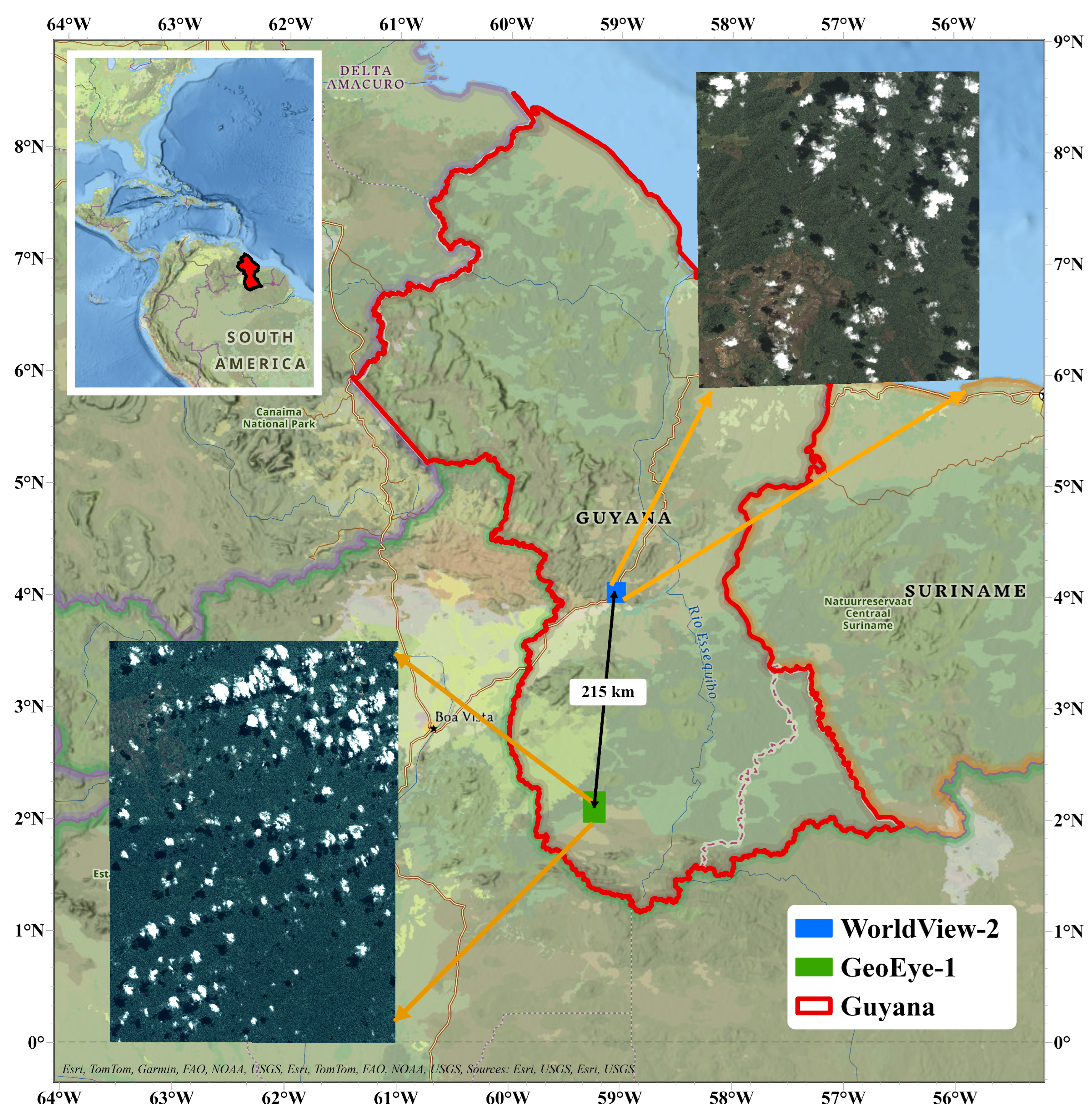
Figure 2.
Example of training sample selection, GeoEye-1 image.
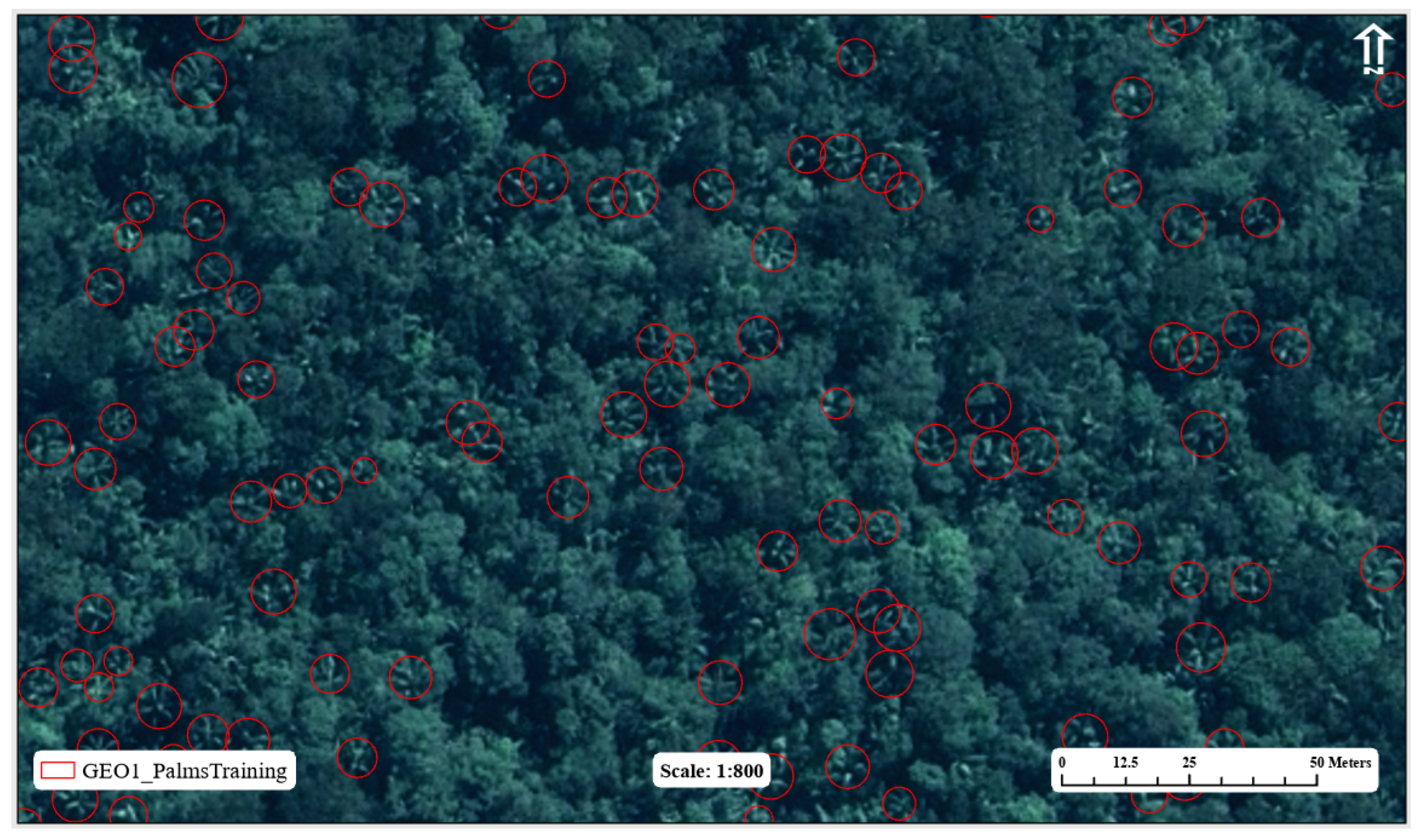
Figure 3.
Workflow diagram for active learning collection of training samples.
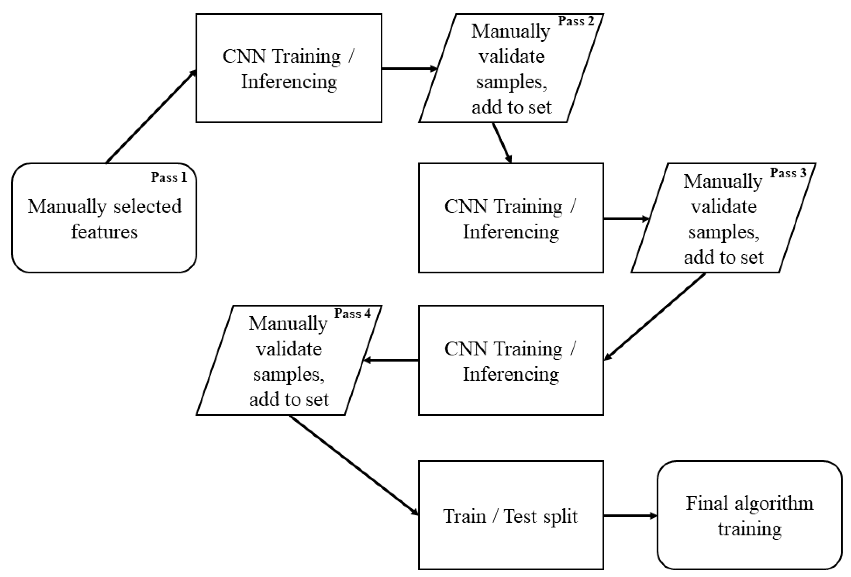
Figure 4.
Train (red square) and Test (blue square) plots for GeoEye-1. NDVI shaded areas indicate clouds, water, or savanna with low likelihood to contain palm features.
Figure 4.
Train (red square) and Test (blue square) plots for GeoEye-1. NDVI shaded areas indicate clouds, water, or savanna with low likelihood to contain palm features.
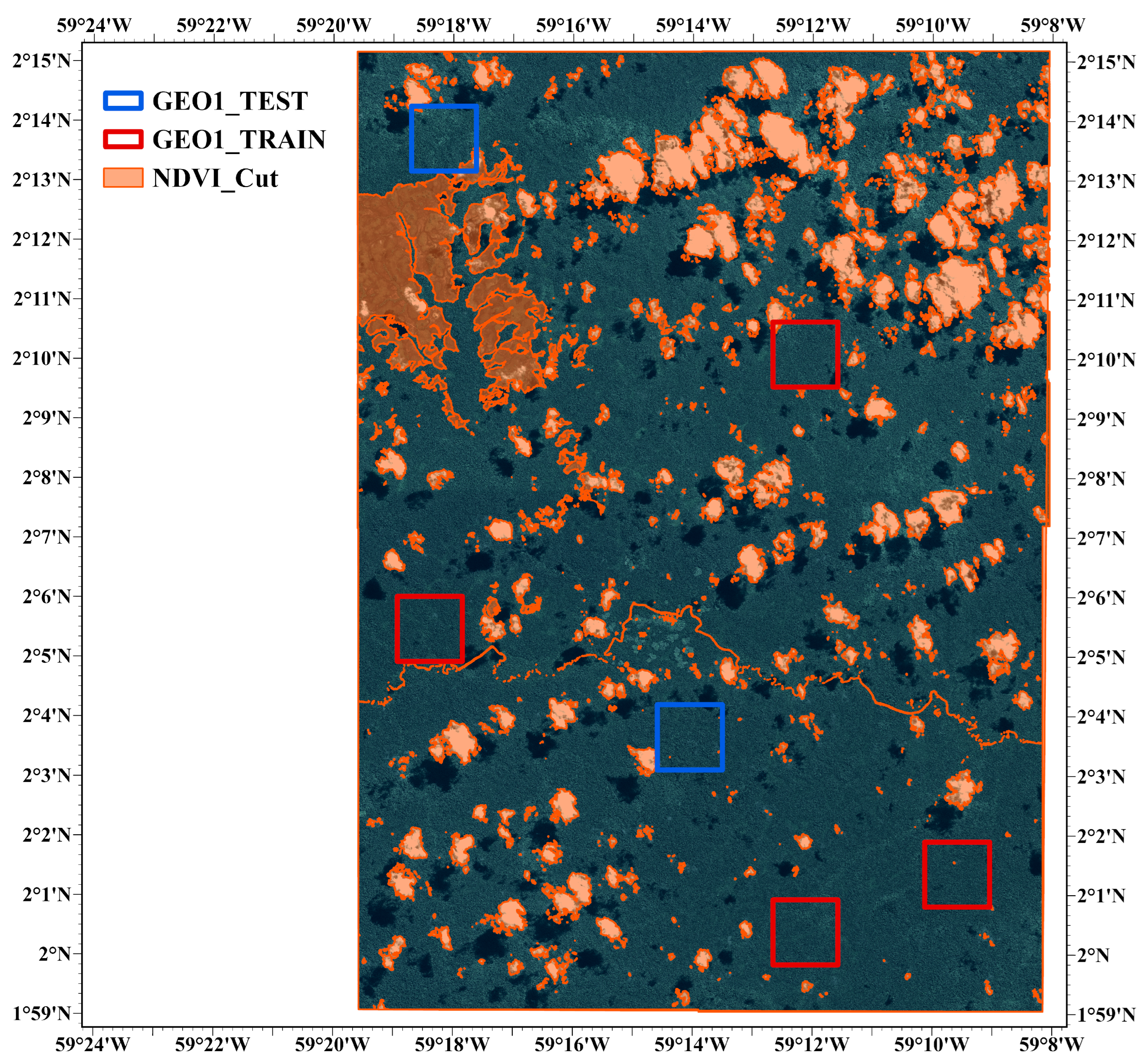
Figure 5.
Intersection over Union
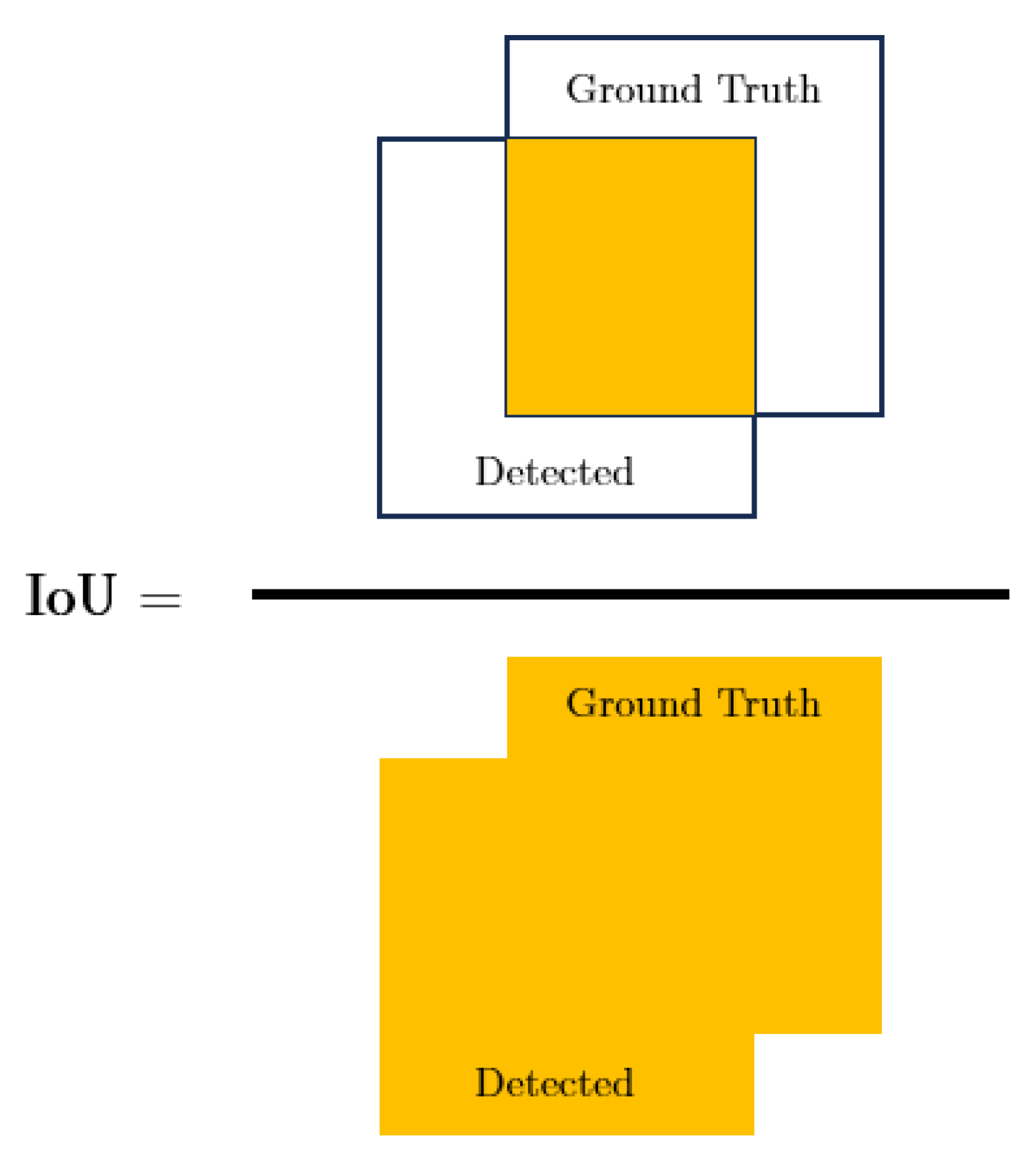
Figure 6.
Confusion matrix. Note that for object detection, True Negative is not a valid class.
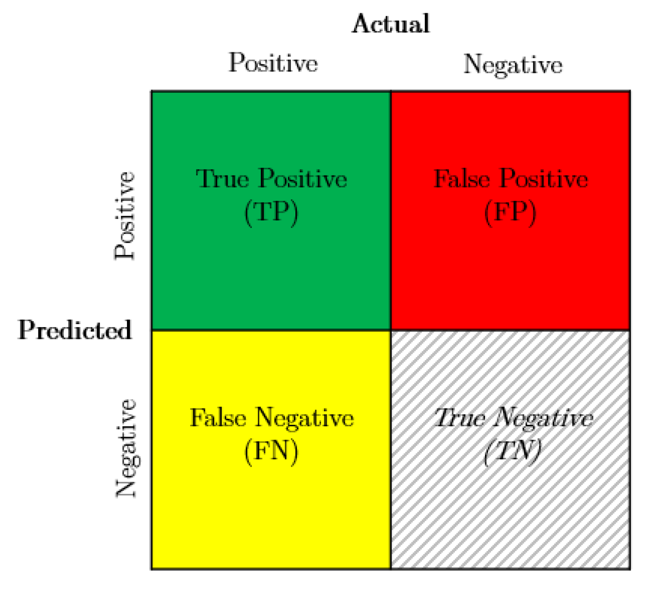
Figure 7.
Training samples (red) overlain by detected features (green). Several examples of error have been notated: false positive (orange arrow) and false negative (pink arrow). Upon closer examination of several instances of false positives, it becomes evident that they are true positive features that were not accounted for during the collection of training data. Overcoming human error or bias can be a challenging obstacle.
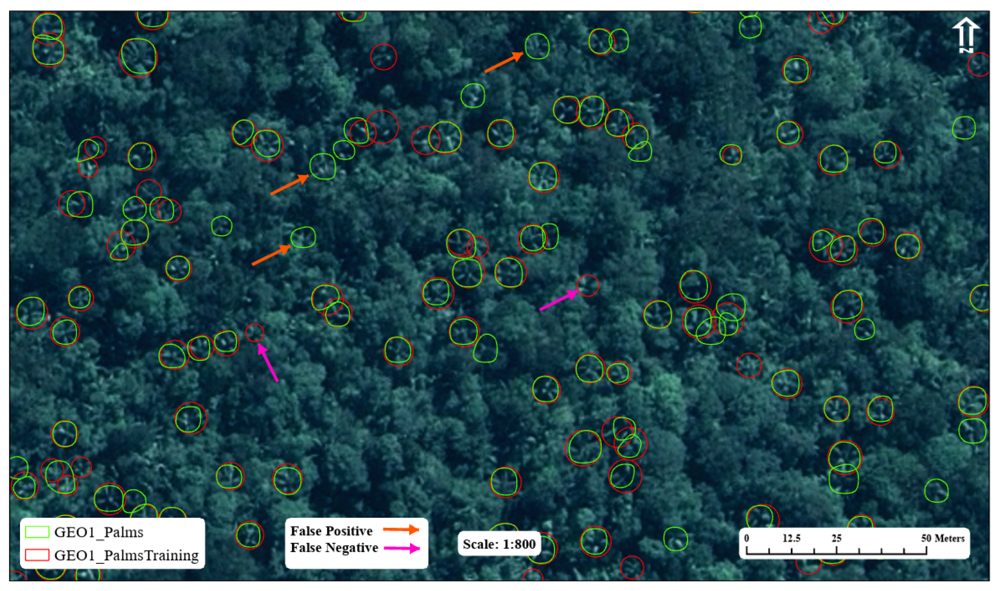
Figure 8.
Palm detection examples, GeoEye-1.
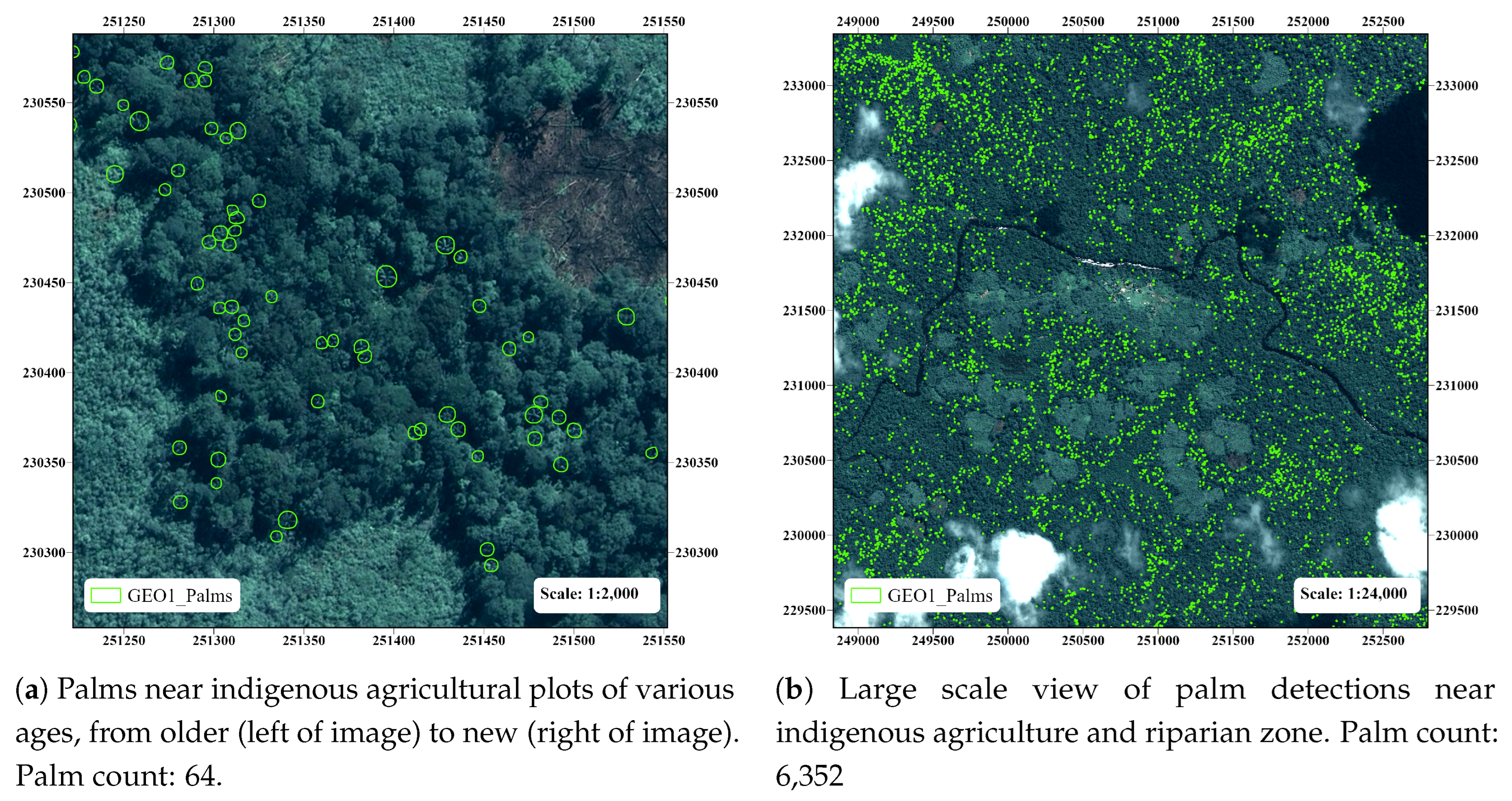
Figure 9.
Train (red square) and Test (blue square) plots for WorldView-2. NDVI shaded areas indicate clouds, water, road, or savanna with low likelihood to contain palm features.
Figure 9.
Train (red square) and Test (blue square) plots for WorldView-2. NDVI shaded areas indicate clouds, water, road, or savanna with low likelihood to contain palm features.
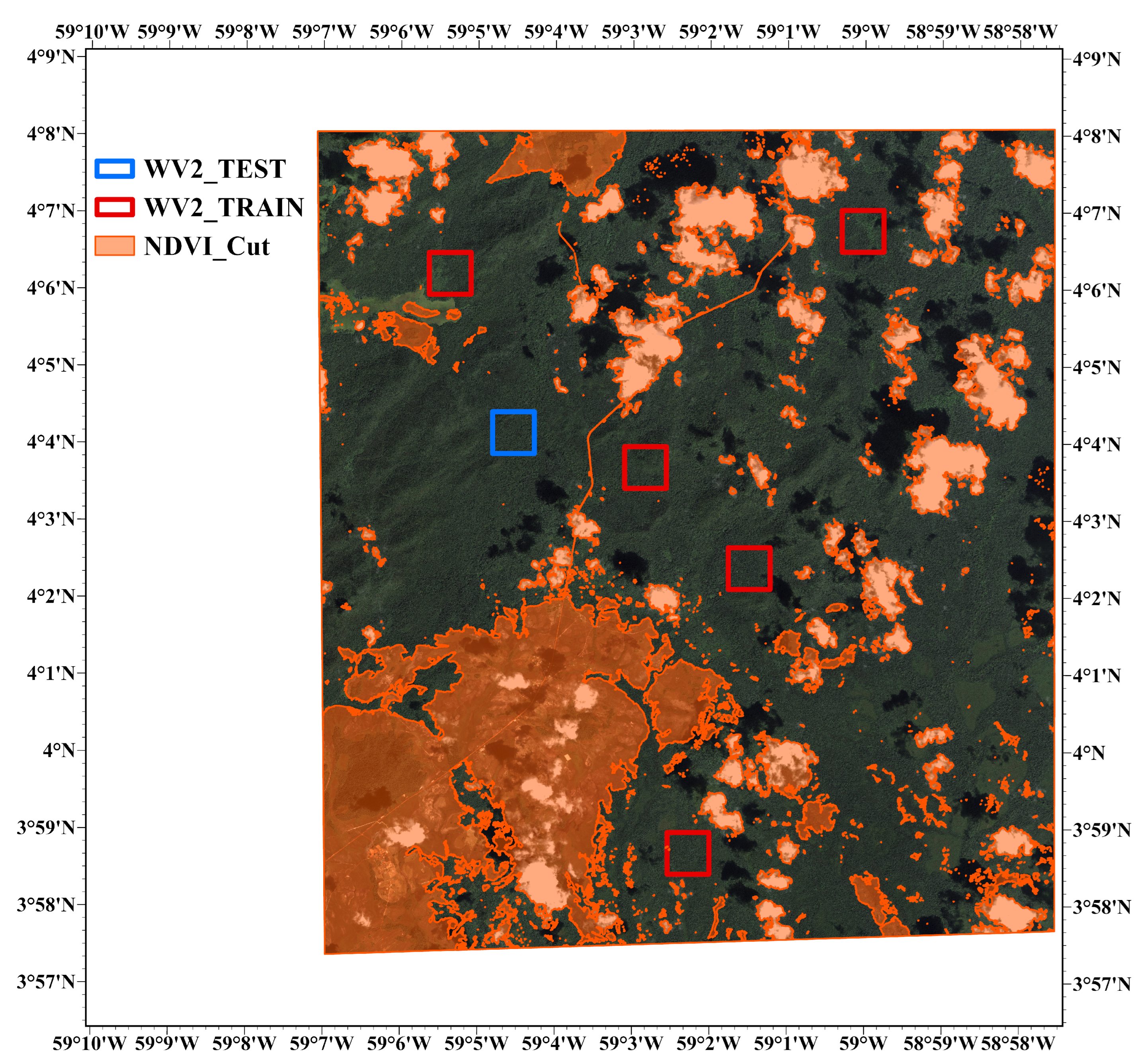
Figure 10.
Palm detection examples, WorldView-2.
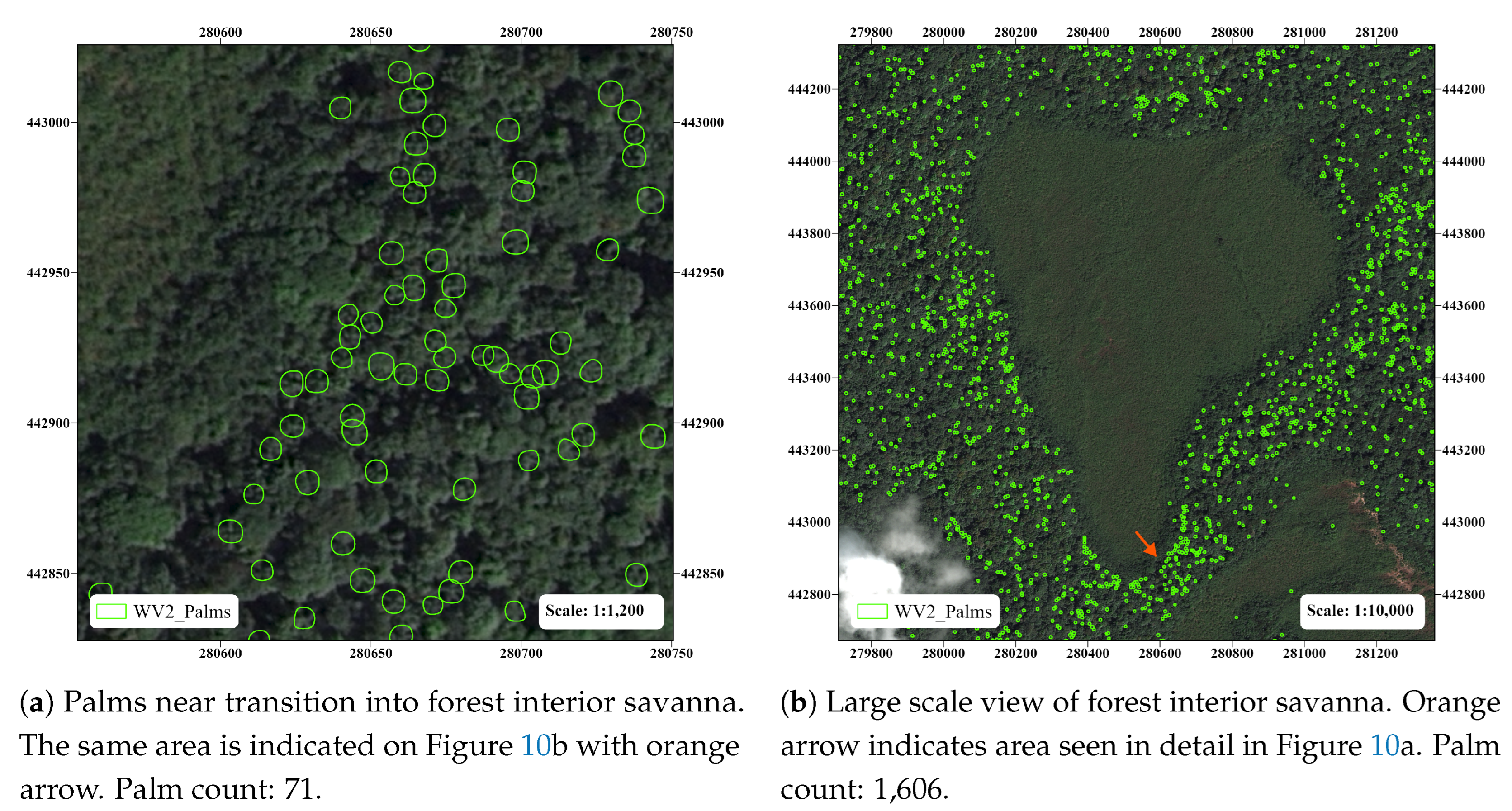
Figure 11.
Graphs showing variation of precision, recall, and F1 with increasing confidence lower boundary. By locating where precision and recall are equal, the optimal confidence threshold is found.
Figure 11.
Graphs showing variation of precision, recall, and F1 with increasing confidence lower boundary. By locating where precision and recall are equal, the optimal confidence threshold is found.
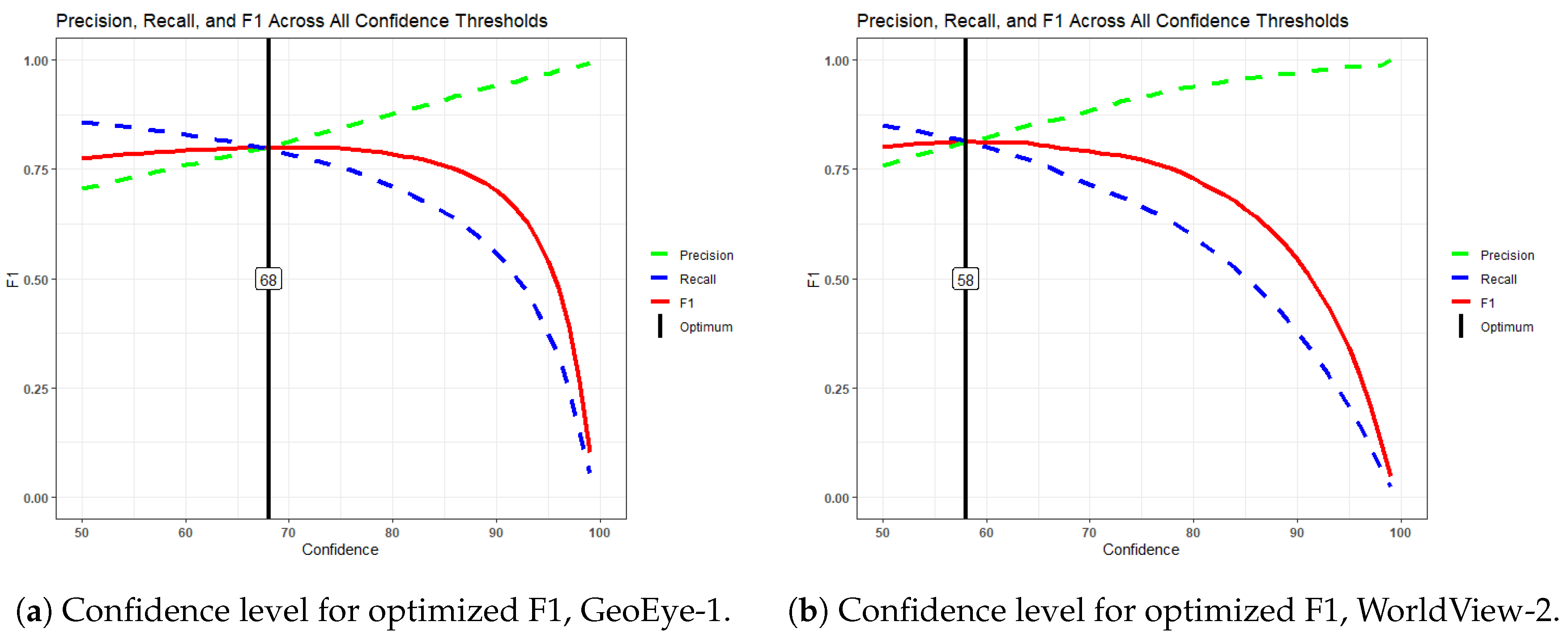
Figure 12.
Example of down-scaling scheme for training sample reduction.
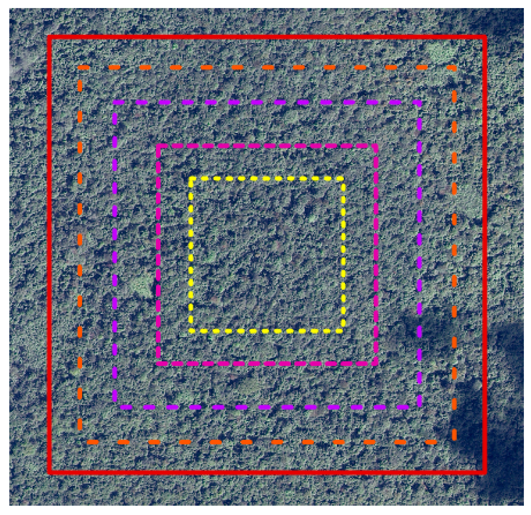
Figure 13.
Training and test set metrics for downscaled sample sets, GeoEye-1. The letter labels align with the ID codes in Table 13. It is important to note that although the performance of train sets d and e seems consistent, there is a noticeable decrease in the model performance on the test sets.
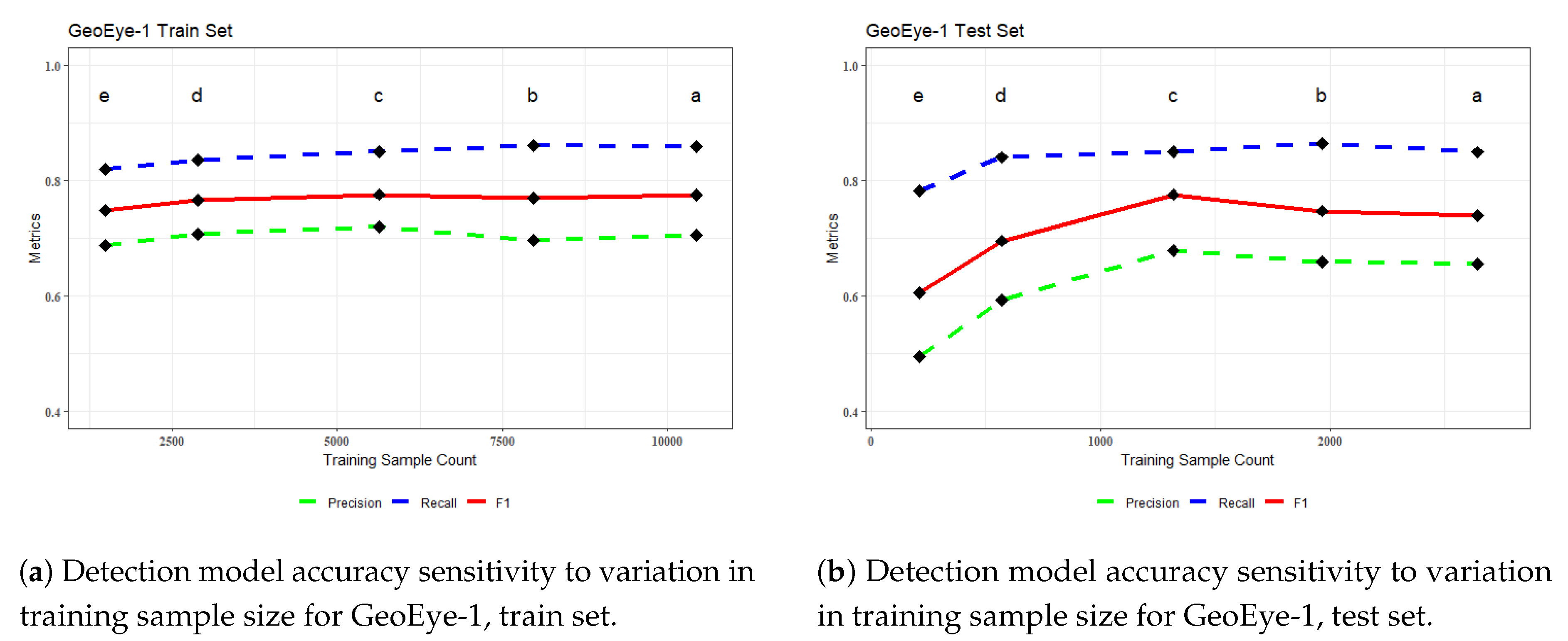
Figure 14.
Training and test set metrics for downscaled sample sets, WorldView-2. The letter labels align with the ID codes in Table 13. Both the training and testing sets show a notable decrease in model performance in subsets d and e.
Figure 14.
Training and test set metrics for downscaled sample sets, WorldView-2. The letter labels align with the ID codes in Table 13. Both the training and testing sets show a notable decrease in model performance in subsets d and e.
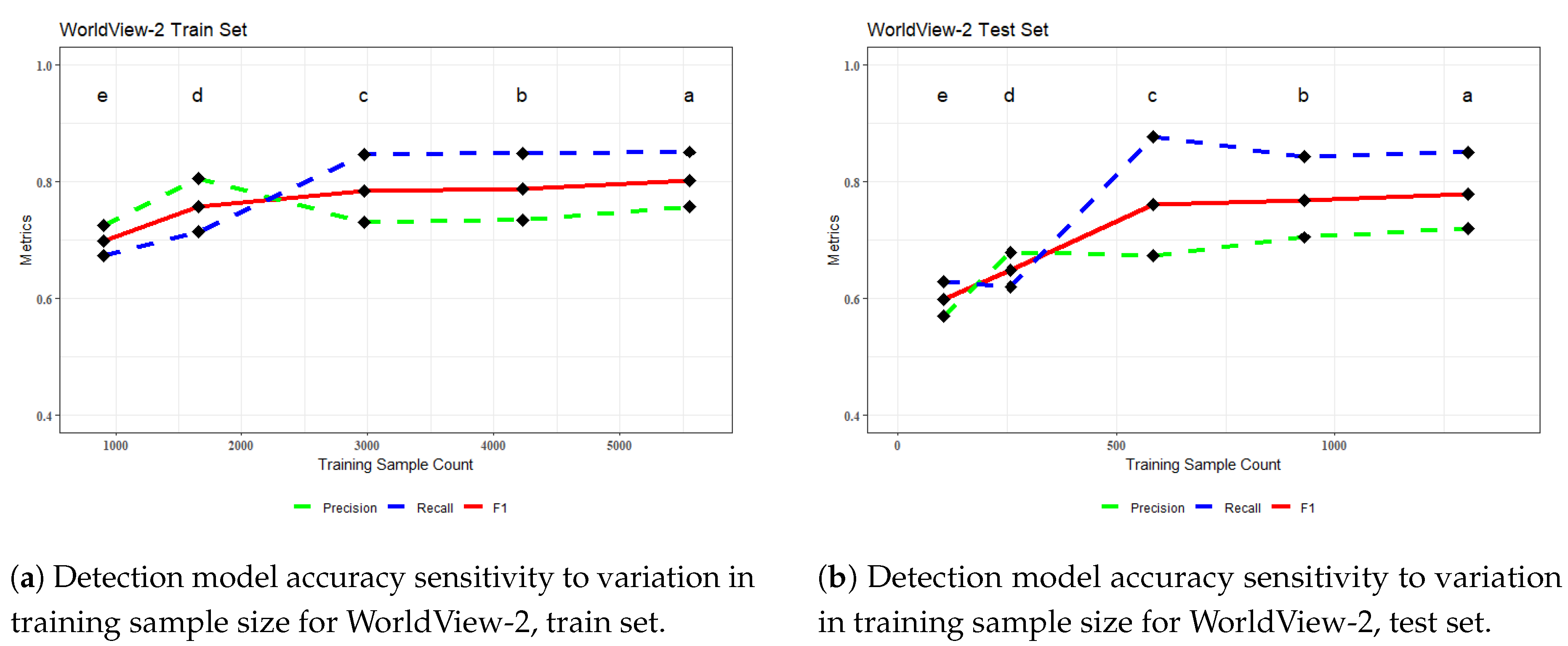
Figure 15.
Palm crown diameter distribution as estimated from mask detection polygons. Examples of crown measurements across the distribution are seen in Figure 16 and Figure 17.
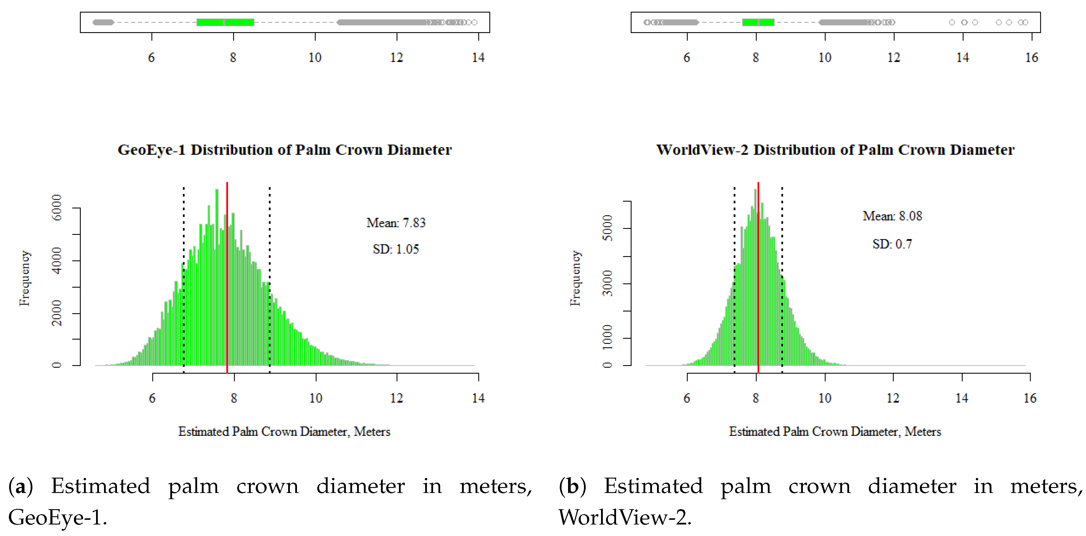
Figure 16.
Example of palms less than or equal to the mean of the crown diameter distribution seen in Figure 15.
Figure 16.
Example of palms less than or equal to the mean of the crown diameter distribution seen in Figure 15.
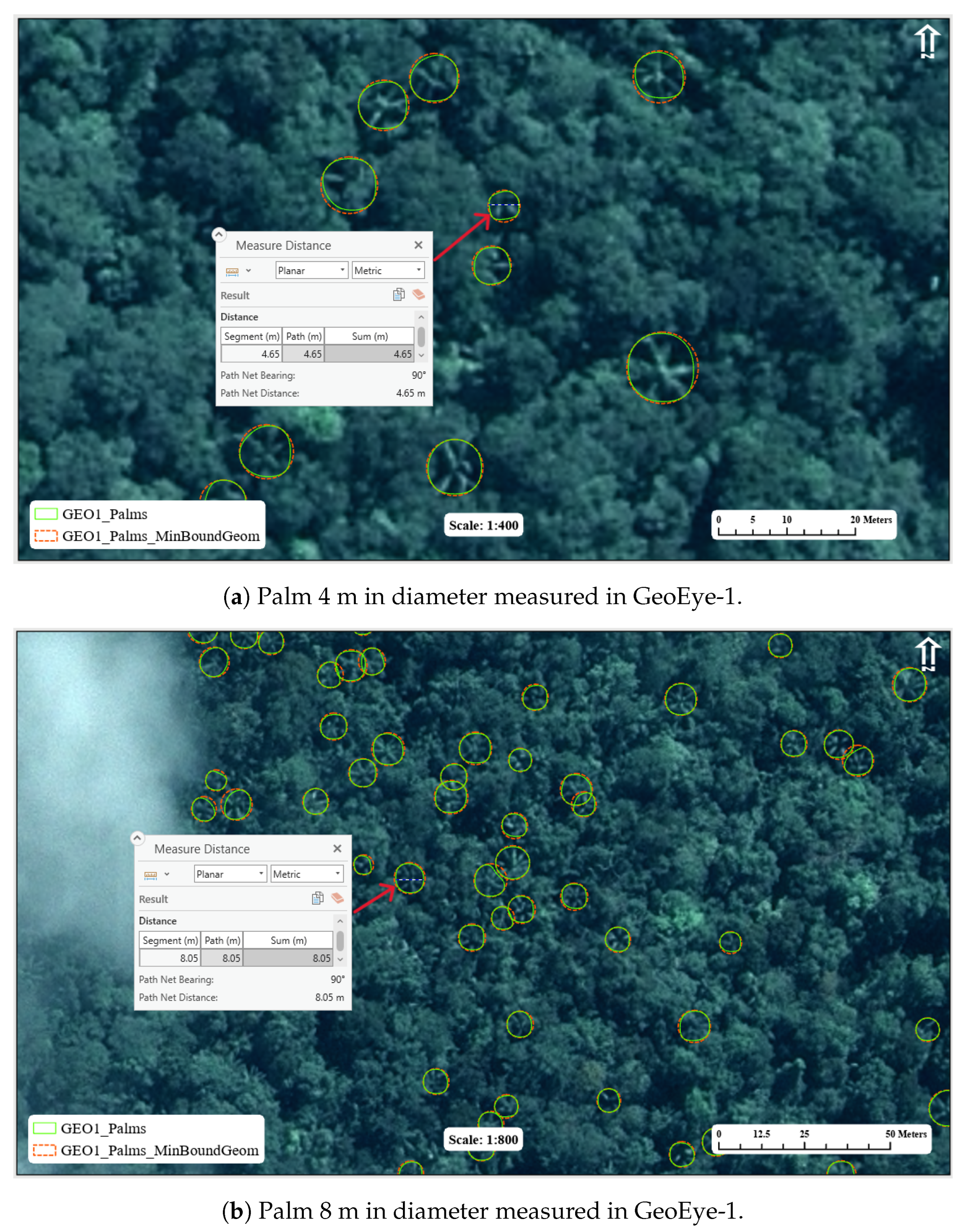
Figure 17.
Example of palms greater than the mean of the crown diameter distribution seen in Figure 15.
Figure 17.
Example of palms greater than the mean of the crown diameter distribution seen in Figure 15.
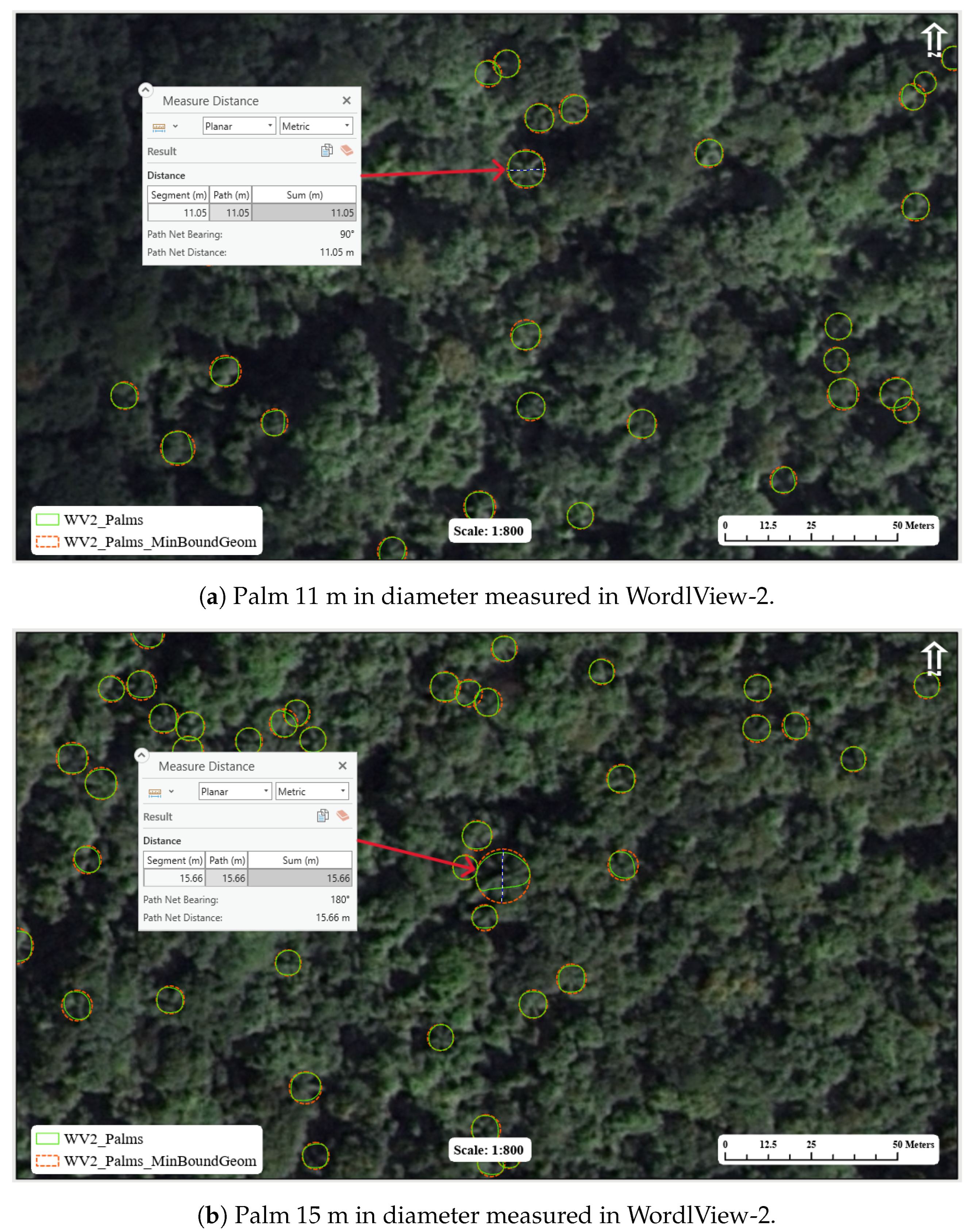
Table 1.
Summary of information for GeoEye-1 and WorldView-2 imagery sets. The net sq km shown in the far right column is estimated using an NDVI cutoff of 0.5 for GeoEye-1 and 0.6 for WorldView-2. This value estimates total area of the image not including clouds, grassland, or bare earth.
Table 1.
Summary of information for GeoEye-1 and WorldView-2 imagery sets. The net sq km shown in the far right column is estimated using an NDVI cutoff of 0.5 for GeoEye-1 and 0.6 for WorldView-2. This value estimates total area of the image not including clouds, grassland, or bare earth.
| Pan GSD | MS GSD | # MS Bands | Bit Depth | # Scenes | Total SqKm | Net SqKm | |
|---|---|---|---|---|---|---|---|
| GeoEye-1 | 0.41m (0.5m pixel) | 1.64m (2.0m pixel) | 4 | 11 | 4 | 637 | 549 (86%) |
| WorldView-2 | 0.46m (0.5m pixel) | 1.80m (2.0m pixel) | 8 | 11 | 9 | 348 | 265 (76%) |
Table 2.
Center point of electromagnetic wavelength for each spectral band in GeoEye-1 and WorldView-2 sensors. WorldView-2 bands matched with GeoEye-1 are in bold font.
Table 2.
Center point of electromagnetic wavelength for each spectral band in GeoEye-1 and WorldView-2 sensors. WorldView-2 bands matched with GeoEye-1 are in bold font.
| GeoEye-1 | WorldView-2 | |||
|---|---|---|---|---|
| Band | Center Wavelength (nm) | Band | Center Wavelength (nm) | |
| Blue | 484 | Coastal | 427 | |
| Green | 547 | Blue | 478 | |
| Red | 676 | Green | 546 | |
| NIR | 851 | Yellow | 608 | |
| Red | 659 | |||
| Red Edge | 724 | |||
| NIR1 | 833 | |||
| NIR2 | 949 | |||
Table 3.
Total number of training samples and relative train-test split.
| Train | Test | |||
|---|---|---|---|---|
| 10,432 | 2,642 | |||
| NTotal = 13,074 | PTrain = 80% | PTest = 20% | ||
Table 4.
Mask R-CNN backbone selection criteria metrics. ResNet-50 and VGG-16 were the top performers with the highest metrics in 4 and 2 categories, respectively. ResNet-50 was selected as the final choice.
Table 4.
Mask R-CNN backbone selection criteria metrics. ResNet-50 and VGG-16 were the top performers with the highest metrics in 4 and 2 categories, respectively. ResNet-50 was selected as the final choice.
| (a) Assessment metrics for the training data set. | ||||||
| Backbone | mAP | AP50 | AP75 | Precision50 | Recall50 | F150 |
| ResNet-101 | 0.418 | 0.748 | 0.444 | 0.578 | 0.851 | 0.689 |
| ResNet-50 | 0.438 | 0.767 | 0.481 | 0.576 | 0.872 | 0.694 |
| ResNeST-101e | 0.339 | 0.642 | 0.329 | 0.492 | 0.779 | 0.603 |
| ResNeST-50d | 0.358 | 0.669 | 0.355 | 0.499 | 0.806 | 0.616 |
| SSL-ResNeXt-101-32x4d | 0.233 | 0.497 | 0.172 | 0.467 | 0.627 | 0.536 |
| SSL-ResNeXt-50-32x4d | 0.229 | 0.484 | 0.178 | 0.481 | 0.602 | 0.536 |
| VGG-16 | 0.419 | 0.746 | 0.452 | 0.635 | 0.828 | 0.719 |
| VGG-13 | 0.396 | 0.720 | 0.414 | 0.630 | 0.803 | 0.706 |
| (b) Assessment metrics for the test data set. | ||||||
| Backbone | mAP | AP50 | AP75 | Precision50 | Recall50 | F150 |
| ResNet-101 | 0.401 | 0.733 | 0.408 | 0.499 | 0.853 | 0.630 |
| ResNet-50 | 0.417 | 0.734 | 0.449 | 0.480 | 0.863 | 0.617 |
| ResNeST-101e | 0.326 | 0.634 | 0.307 | 0.389 | 0.800 | 0.523 |
| ResNeST-50d | 0.334 | 0.645 | 0.316 | 0.386 | 0.804 | 0.522 |
| SSL-ResNeXt-101-32x4d | 0.210 | 0.471 | 0.141 | 0.413 | 0.605 | 0.491 |
| SSL-ResNeXt-50-32x4d | 0.206 | 0.451 | 0.149 | 0.381 | 0.594 | 0.464 |
| VGG-16 | 0.388 | 0.723 | 0.382 | 0.539 | 0.827 | 0.652 |
| VGG-13 | 0.370 | 0.697 | 0.360 | 0.526 | 0.804 | 0.636 |
Table 5.
Confusion matrix values for default Mask RCNN model, training set. At this stage, false negatives are in very high proportion to true positives.
Table 5.
Confusion matrix values for default Mask RCNN model, training set. At this stage, false negatives are in very high proportion to true positives.
| Ground Truth | |||
|---|---|---|---|
| Positive | Negative | ||
| Detection | Positive | 9,091 | 6,693 |
| Negative | 1,338 | - | |
| 2-4 | |||
Table 6.
GeoEye-1 confusion matrices and accuracy metrics for final inference after model tuning. This shows a 44% reduction in false negative detections from the baseline model.
Table 6.
GeoEye-1 confusion matrices and accuracy metrics for final inference after model tuning. This shows a 44% reduction in false negative detections from the baseline model.
| (a) Confusion matrix values for final inference output, train set. | ||||
| Ground Truth | ||||
| Positive | Negative | |||
| Detection | Positive | 8,956 | 3,754 | |
| Negative | 1,473 | - | ||
| (b) Confusion matrix values for final inference output, test set. | ||||
| Ground Truth | ||||
| Positive | Negative | |||
| Detection | Positive | 2,243 | 1,184 | |
| Negative | 399 | - | ||
Table 7.
WorldView-2 training samples and relative train / test split.
| Train | Test | |
| 5,551 | 1,304 | |
| NTotal = 6,855 | PTrain = 81% | PTest = 19% |
Table 8.
WorldView-2 confusion matrices and accuracy metrics using same CNN model parameters as in GeoEye-1, with image specific training samples.
Table 8.
WorldView-2 confusion matrices and accuracy metrics using same CNN model parameters as in GeoEye-1, with image specific training samples.
| (a) Confusion matrix values for final inference output, training set. | ||||
| Ground Truth | ||||
| Positive | Negative | |||
| Detection | Positive | 4,722 | 1,517 | |
| Negative | 829 | - | ||
| (b) Confusion matrix values for final inference output, test set. | ||||
| Ground Truth | ||||
| Positive | Negative | |||
| Detection | Positive | 1,108 | 433 | |
| Negative | 196 | - | ||
Table 9.
GeoEye-1 palms inference metrics at F1 optimized confidence lower boundary of 68%. Subscripts refer to minimum IoU, not confidence level.
Table 9.
GeoEye-1 palms inference metrics at F1 optimized confidence lower boundary of 68%. Subscripts refer to minimum IoU, not confidence level.
| (a) Confusion matrix values for training set at > 68% confidence. | ||||
| Ground Truth | ||||
| Positive | Negative | |||
| Detection | Positive | 8,307 | 2,064 | |
| Negative | 2,122 | - | ||
| (b) Confusion matrix values for test set at > 68% confidence. | ||||
| Ground Truth | ||||
| Positive | Negative | |||
| Detection | Positive | 2,053 | 626 | |
| Negative | 589 | - | ||
Table 10.
WorldView-2 palms inference metrics at F1 optimized confidence lower boundary of 58%. Subscripts refer to minimum IoU, not confidence level.
Table 10.
WorldView-2 palms inference metrics at F1 optimized confidence lower boundary of 58%. Subscripts refer to minimum IoU, not confidence level.
| (a) Confusion matrix values for training set at > 58% confidence. | ||||
| Ground Truth | ||||
| Positive | Negative | |||
| Detection | Positive | 4,518 | 1,048 | |
| Negative | 1,033 | - | ||
| (b) Confusion matrix values for test set at > 58% confidence. | ||||
| Ground Truth | ||||
| Positive | Negative | |||
| Detection | Positive | 1,049 | 298 | |
| Negative | 255 | - | ||
Table 11.
Comparison of confusion matrix values and net palm count with confidence of >50% and >68% for GeoEye-1.
Table 11.
Comparison of confusion matrix values and net palm count with confidence of >50% and >68% for GeoEye-1.
| Train | Test | |||||||
|---|---|---|---|---|---|---|---|---|
| Confidence | >50% | >68% | % | >50% | >68% | % | ||
| True Positive | 8,956 | 8,307 | -649 | -7% | 2,243 | 2,053 | -190 | -8% |
| False Positive | 3,754 | 2,064 | -1,690 | -45% | 1,184 | 626 | -558 | -47% |
| False Negative | 1,473 | 2,122 | 649 | 44% | 399 | 589 | 190 | 48% |
| Gross Count | 278,270 | 223,458 | -54,812 | -20% | ||||
Table 12.
Comparison of confusion matrix values and net palm count with confidence of >50% and >58% for WorldView-2.
Table 12.
Comparison of confusion matrix values and net palm count with confidence of >50% and >58% for WorldView-2.
| Train | Test | |||||||
|---|---|---|---|---|---|---|---|---|
| Confidence | >50% | >58% | % | >50% | >58% | % | ||
| True Positive | 4,722 | 4,518 | -204 | -4% | 1,108 | 1,049 | -59 | -5% |
| False Positive | 1,517 | 1,048 | -469 | -31% | 433 | 298 | -135 | -31% |
| False Negative | 829 | 1,033 | 204 | 25% | 196 | 255 | 59 | 30% |
| Gross Count | 194,483 | 166,927 | -27,556 | -14% | ||||
Table 13.
Values for train-test sets after downscaling.
| GeoEye-1 | WorldView-2 | |||||
|---|---|---|---|---|---|---|
| ID | AreaHa | NTrain | NTest | AreaHa | NTrain | NTest |
| a | 400 | 10,432 | 2,642 | 100 | 5,551 | 1,304 |
| b | 300 | 7,968 | 1,965 | 75 | 4,227 | 931 |
| c | 200 | 5,635 | 1,317 | 50 | 2,970 | 585 |
| d | 100 | 2,888 | 569 | 25 | 1,659 | 258 |
| e | 50 | 1,480 | 211 | 12.5 | 901 | 105 |
Disclaimer/Publisher’s Note: The statements, opinions and data contained in all publications are solely those of the individual author(s) and contributor(s) and not of MDPI and/or the editor(s). MDPI and/or the editor(s) disclaim responsibility for any injury to people or property resulting from any ideas, methods, instructions or products referred to in the content. |
© 2024 by the authors. Licensee MDPI, Basel, Switzerland. This article is an open access article distributed under the terms and conditions of the Creative Commons Attribution (CC BY) license (http://creativecommons.org/licenses/by/4.0/).
Copyright: This open access article is published under a Creative Commons CC BY 4.0 license, which permit the free download, distribution, and reuse, provided that the author and preprint are cited in any reuse.


