

Submitted:
13 November 2024
Posted:
14 November 2024
You are already at the latest version
Abstract
The residential minimum water demand characterization is of fundamental importance for water distribution systems management. During the minimum consumption, indeed, maximum pressures are on network pipes and at the same time tank levels rise. The legitimate water consumption analysis during period of low demand and high pressure is thus of great interest for leakages estimation due to the increase of the water loss with the pressure. Previous studies have tackled this issue with deterministic approaches, by considering the legitimate consumption as a percentage of the night measured inflow. In order to contributing to the legitimate minimum residential water demand characterization, probabilistic models have been developed to study and forecast the daily minimum residential water demand. Some probability distributions have been tested by means of statistical inferences on data set collected from different District Metering Areas (DMAs), showing the stochastic minimum flow demand is described by the log-Normal (LN), Gumbel (Gu) and Log-Logistic (LL) distributions, as an extreme minimum value. The latter is of particular interest being the LL probability density function analytically integrated. With reference to the analysed DMAs, parameters of such statistical distributions have been estimated and relationship are provided in function only of the supplied users for different DMAs. Data have been analysed with 1 h interval time of discretization, with the aim of providing an useful guide to the Water Utilities which usually are managing water distribution systems data with such resolution time. Indeed, once the legitimate minimum residential flow consumption at 1h interval time is estimated in function of the users number, by subtracting it to the inflow measured, it is possible to estimate leakages rate at the DMA.
Keywords:
minimum residential water demand
; MNF
; leakages
; probabilistic analysis
; Logistic distribution
; WDS
; DMA
1. Introduction
Minimum water demand characterization is of fundamental importance for Water Distribution Systems (WDS) management, being the lower residential consumption responsible of higher pressures on the system pipes (and then of increased leakages) and of increase of tank levels.
Several methodologies (e.g., [1,2,3]) are available in the literature for supporting WDS management in leakages quantity estimation.
An usual approach for leakages assessment is the minimum night flow (MNF) method (e.g. [4,5,6]). It is based on detecting leakages in a network by subtracting at the inflow data the users night legitimate consumption. Usually, in residential areas, the balance refers at night time - between 02:00 and 04:00 a.m. hours (e.g. [7]) – being the period of the day in which residential water consumption is minimum and high leakages occur.
However, the accuracy in leakages estimation strongly depends on the accuracy of legitimate night flow consumptions. The knowledge of the legitimate minimum residential consumption, thus, is of great interest for the leaks quantification, being usually known from the water companies solely the total flow supplied to the urban area during the different time of the day.
Because of this interest, several approaches in the literature aimed at estimating the MNF, usually assuming the residential legitimate consumption as a given percentage of the total flow. Most of them are analyzing the possible legitimate consumption from users by summing the amount of L/h used by the single apparatus (i.e. flushing toilets, etc..) and estimating a sum of them in function of the number of possible taps opened at night time (e.g. [8,9,10,11]). The so detected MNF value, however, resulted in some cases too low respect to the real legitimate night flow consumption (e.g. [11]) even when contributions are based on measurements carried out with high temporal frequency, minutes respect to hours, leading to an overestimation of leakages.
Some other approaches (e.g. [12]) highlight the importance of analyzing high resolution data, even at 1 second time sampling interval, for a more realistic characterization of water losses. This assumption is also more necessary at the increasing of users number.
The study of the water demand of aggregate users, as in the case herein proposed for the MNF, requires a trade-off between the need of characterize the water requirement as close as possible to the real consumption by considering a shortest interval time and the need of recording and collecting a big amount of data from Water Utilities. Several contributions (i.e. [13,14,15,16]) are reporting the incidence of the interval time of discretization (ΔT) on the water demand estimation. In reference to the maximum peak condition, Tricarico et al. [17] observed that when the time step is equal to 1 h, the peak demands are underestimated around the 20% for ΔT=1 min. Gargano et al [14] determined a corrective coefficient for estimating the peak value at varying the time interval. Tricarico et al. [18] and Gargano et al. [19] showed the importance of considering a short interval time, ranging among 1-10 min, for studying the probability of null water demand (F0) in reference to a number of users ranging in between 500-1250, being for greater intervals the F0 almost null. Indeed, Buchberger and Nadimpally [12] demonstrated that the probability of null request decreases exponentially with the increasing ΔT.
However this accuracy in reality is a very difficult task. Water Utilities are not equipped with flow and pressure measurement instruments able to reach constantly this level of accurateness. Indeed, despite of this, Water Companies, have the need to manage a big amount of data and then the assumed sampling interval time is usually of the order of 1 h, in particular due to problems related to data transmission. In order of modelling the water demand for practical application, thus, it is necessary to estimate and characterize the water demand at hourly time step. In this case it will be almost impossible, even for the lower number of users of the examined range, to detect an hour of the day in which there is the probability that a user is not requiring water, even more when the number of users increases.
The latter is the reason for which, it is of fundamental importance the WDS division into Measurement Districts Areas (DMAs) (e.g. [20,21,22]). This methodology, originally developed in the UK (e.g. [23]) and already implemented in many countries, consists of partitioning a water system into subsystems (called ‘districts’) delimited by control valves (physical district) or by flow meters (virtual district) in which the water balance calculation is simplified and referred to a lower number of users respect to the whole WDS.
Under this assumption, this work aims to contribute to the characterization of the legitimate minimum flow consumption by analyzing with a probabilistic approach real water consumption data recorded with a mean of 1 h interval time in 14 DMAs realized on real WDS in Campania Region, Italy. Real data are analysed in order to investigate the relationship between the MNF and the DMA characteristics, first of all the number of users.
With reference to the analysed DMAs, parameters of such statistical distributions have been estimated and relationship are provided in function only of the supplied users for different DMAs. The generalization of obtained relationships can improve the capability of estimating water losses in a DMA by means of the MNF method and then to perform strategies for water losses reduction.
2. Case Studies and Demand Data Analysis
The DMAs considered in this study (Figure 1) are characterized by a users number (Nusers) ranging about 600 to 17000. Data are recorded continuously with a mean interval time of 1 h and they are referring to the winter period, from September to February, and to solely weekly days. This choice has been done because of the need of analyzing the minimum effective night consumption at residential level without it could be influenced by seasonal temperature variability or by the different residential behavior during the weekends or holidays periods. However, because of leakages variability with the time, solely 30-35 continuous days for each DMA have been examined for the MNF estimation, because characterized by the absence of variation in leakages due to structural works done from Water Utilities.
The analysed DMAs were characterized by an high leakage level due also to the high pressures present in the systems. Because of this, Water Utility introduced in some districts Pressure Reduction Valves (PRV) and carried on a water leaks search and reduction campaign. In the DMAs analysed, flow and pressure measurements were simultaneously performed, and this allowed the estimation of the time variation of the water loss. A deep study on the flow-pressure data has been done in order to estimate the leaks value in the analysed period and their daily patterns, which varies with the pressure regulation value. The PRV is regulating the pressures over the 24 hours of the day, by reducing them during the night time. The result of this is evident in the plots of Figure 2 in which the losses flow is lower during the night time than the daily one.
The same procedure has been undertaken also for DMAs in which the PRV is not present but a measure of pressures at each t interval time [h] is available (Figure 3). In these cases, as expected, the losses flow during the night is higher than during the day time, not being the pressures regulated by a PRV.
The consideration of leakages variation in function of the pressures has been demonstrated, in the examined case studies, of particular relevance in order to detect the water losses accurately. In fact, it is not possible to consider the water losses constant and equal to the mean leakages value in case of PRV regulation being the night water loss reduced and in case of DMAs without regulation, as shown in Figure 3, it could lead to an underestimation of the leakages during the night and an overestimation of leakages during the day.
Data recorded have been thus cleaned from the physical leakages in order to estimate the effective water demand by users.
Water demand has been dimensionless represented by means of the demand coefficient CD (t):
where is the mean water demand of the examined period and the value of water demand at time t.
Hence in Paragraph 3 statistics of the residential minimum consumption are referred to the dimensionless random variable of Equation (1).
In particular, the night consumption, at difference from leakages, could be considered as a random variable, changing in function of the needs of the residential users and not solely with the pressure. Under this assumption a probabilistic approach has been undertaken.
3. MNF Probabilistic Distributions
The extreme events, as the minimum night consumption, are effectively described by means of asymmetric distributions (e.g. [24]), as for instance the Log-Normal distribution (LN) that has the following - probability density function (pdf):
or the pdf of Gumbel distribution (Gu):
where: x is the random variable and y = lnx; the symbols μ and σ represent respectively the mean and the standard deviation. The parameters α and ε of Gu are given by the relations:
and the Log-Logistic (LL) model, which presents a trend very similar to the LN, but contrary to Gauss model, the probability density function can be analytically integrated ([25,26]). The CDF of the LL distribution has the following expression:
if x = Cdmin (dimensionless minimum demand Equation (1)), y is lnCdmin.
The parameters of Equation (5) can be estimated by means of statistics on the logarithmic of the original sample, or by means of μ and σ of the pristine random variable by means of the following equations ([25]):
where CVx = σx/μx is the variation coefficient.
All the suggested distributions are defined for the Cdmin>0. The choice of taking into account bi-parametric models has been guided by the need to find models that lead reliable estimation of few parameters and thus provide themselves to a practical application.
The LN, Gu and LL distributions have been tested by means of the observed data for the different DMAs, assuming a time aggregation ∆T = 1 h.
The diagrams in Figure 4 are the Quantile-Quantile (Q-Q) plots for the monitored number of users. The Q-Q plots show the comparison between the observed and the theoretical Cdmin quantiles with the same probability of occurrence. The theoretical values were estimated by means of the integral of Equations (2) and (3) -numerical integration for LN distribution- and Equation (5). The quantiles of the minimum demand of Figure 4 fit well the bisector line, which represents the condition where the observed quantiles are equal to the theoretical quantiles.
The effectiveness of the three distributions was checked by means of the Kolmogorov-Smirnov (KS) test. Figure 5 summarizes the threshold values for a 1% confidence level (D1% - reported with the dot line) and the relative KS parameters (D) for the LN, Gu and LL CDFs. The fit tests were satisfied (D<D1%) for all monitored users.
In Table 2 the statistics of the data sample (μCdmin and σCdmin) for the different DMA at varying the user number are reported.
As it is of evidence, all the examined distributions proved to be equally effective in modelling the night flow demand.
Equations (2) and (3) allow to explicit the Minimum Demand Coefficient for a predefined probability Pr[S] of not exceedance or (1- Pr[S]) of exceedance. Hence the MNF coefficient with a predefined probability of not exceedance following LL is given by:
while, for Gu distribution, presents the following relation:
The quantile for LN model can be estimated only by means of a numerical approximation.
4. Estimation of Parameters
All the proposed distributions (LN, Gu and LL) are bi-parametric models, hence they require the estimation of two parameters, as the mean and the variation coefficient (CV).
The mean value of the minimum CD recorded in each day of the examined period () has been plotted at varying the users number (Nusers), i.e. for the different DMAs analysed, and it is reported in Figure 6.
The minimum demand coefficient is increasing with the number of users, as it was expected. For the analysed DMAs, the experimental data show the trend proposed in relationship (9):
The proposed relationship can allow the estimation of the legitimate users night flow consumption, by knowing only the mean inflow at the DMA and the number of users.
The CV of the minimum night data, CVCdmin, can also be estimated in function of the number of users:
CV experimental points reported in Figure 7 are well fitted by the proposed (10) relationship, which shows, as expected, a decreasing trend of the CV with the users number. It needs to be highlited that CV experimental points tend to 0.1 at the increase of users number, as of evidence also in other residential water demand analyses (e.g. [14,17,19]).
By means of Equations (9) and (10), the parameters of and are estimated solely in function of the DMA number of users.
By the application of Equations (7) and (8) however it is possible to define the MNF with an assigned probability of success/failure. In Figure 8 the confidence intervals for the are reported for predefined probabilities.
At increasing the probability of not exceedance, the value is increasing leading to a greater MNF coefficient and this is more evident at decreasing the number of users. The choice of which probability considered is usually made by the decision maker in function of the problem and as a consequence of a cost-benefit analysis.
The proposed relationships for the models parameters estimation (Equations (9) and (10)) have been then used as a test for evaluating the CDF of data by only knowing the number of users. In Figure 9, the CDF estimated by means of the Gumbel distribution application is compared with the observed one obtaining a good fit in the data representation.
5. Conclusions
The study of the residential minimum water demand is of fundamental importance in WDS management and in leakages estimation. Indeed, the knowledge of the legitimate minimum residential consumption could be also of great interest for the leaks quantification, being usually known from the water companies solely the total volume supplied to the urban area during a specific period of time. The MNF characterization has been herein investigated on 14 different DMAs of Campania Region, in Italy, with a number of users ranging in between 600-17000. Winter weekly water demand data at hourly time step have been analysed and the hourly minimum consumption at varying the users number has been probabilistically modelled. The choice of representing the results with an interval time of 1 h is due to the aim of providing a practical application for the proposed methodology being usually data collected from the Water Companies at hourly time step.
By means of statistical inferences on data set collected from different District Metering Areas (DMAs), the effectiveness of log-Normal (LN), Gumbel (Gu) and Log-Logistic (LL) distributions has been demonstrated. The latter is of particular interest being the LL probability density function analytically integrated. For the DMAs and the number of users investigated, relationship of the model parameters have been proposed in function of the number of users supplied. The advantage of using the proposed relationships undoubtedly lies in their simplicity, even if probabilistically based. Indeed, in order to estimate the legitimate minimum water consumption from residential users it is necessary to know solely the number of users supplied and the daily mean value of flow requested by the DMA.
The results should be considered valid for the range of users examined in this research, with a residential characteristic and indoor water use. In future works it would be desirable to extend the analysis to a greater number of DMAs.
Author Contributions
Conceptualization, C.T.; methodology, C.T., C.C. and A.L.; validation, C.T., C.C., A.L. and G.d.M.; formal analysis, C.T., C.C. and A.L.; investigation, C.T., C.C. and A.L.; data curation, C.T., C.C. and A.L.; writing—original draft preparation, C.T.; writing—review and editing, C.T., C.C. and A.L.; visualization, C.T., C.C., A.L. and G.d.M.; supervision, C.T. and A.L.; funding acquisition, A.L. All authors have read and agreed to the published version of the manuscript.
Funding
Part of the research presented in the paper was funded under the National Grant PRIN2022 n.2022JN9YNJ "SMART REhabilitation of NEtworks with high Water losses (SMART RENEW)". Cristian Cappello was fully funded in the framework of the Project “PURSIE- Studio Progettazione e Sviluppo di un nuovo modello finalizzato alla gestione del bilanciamento del consumo di acqua nell'ambito di un Programma Urbano di Riduzione degli Sprechi Idrici ed Energetici”, financed by the Italian Ministery of Economic Development - Fondo per la Crescita Sostenibile - Sportello "Fabbrica Intelligente" PON I&C 2014-2020, D.M. 5 marzo 2018 Capo III.
Conflicts of Interest
The authors declare no conflicts of interest. The funders had no role in the design of the study; in the collection, analyses, or interpretation of data; in the writing of the manuscript; or in the decision to publish the results.
Abbreviations
| Variation coefficient of Minimum demand coefficient | |
| CD (t) | Demand coefficient at time t |
| CDF | (acronym) Cumulative Distribution Function |
| Cdmin | Minimum demand coefficient |
| CV | Variation coefficient |
| CVx | Variation coefficient of random variable |
| DMA | (acronym) Demand Monitoring Area |
| Probability density function | |
| Fx | CDF of random variable |
| Gu | (acronym) Gumbel distribution |
| KS | (acronym) Kolmogorov Smirnov test |
| LL | (acronym) Log Logistic |
| LN | (acronym) Log-Normal distribution |
| MNF | Minimum night flow |
| Nusers | Number of users |
| Probability density function | |
| PRV | Pressure reducing valve |
| WDS | (acronym) Water Distribution System |
| x | [depending on variable] Random variable |
| y | [depending on variable] lnx |
| α | Gumbel parameter |
| ∆T [T] | Time step |
| ε | Gumbel parameter, mode |
| μ | Mean |
| Minimum demand coefficient mean | |
| [L/s] | Mean daily water demand |
| σ | [depending on variable] standard deviation |
References
- Puust, R.; Kapelan, Z.; Savic, D.A.; Koppel, T. ; A review of methods for leakage management pipe networks. Urban Water Journal 2010, 7, 25–45. [Google Scholar] [CrossRef]
- Mutikanga, H.E.; Sharma, S.K.; Vairavamoorthy, K. ; Methods and Tools for Managing Losses in Water Distribution Systems. J. of Water Resource. Plann. and Management 2013, 139, 166–174. [Google Scholar] [CrossRef]
- Mazzolani, G.; Berardi, L.; Laucelli, D.; Simone, A.; Martino, R.; Giustolisi, O. ; Estimating Leakages in Water Distribution Networks Based on Inlet Flow Data. Journal of Water Resources Planning and Management, ASCE 2017, 143, 04017014–1-11. [Google Scholar] [CrossRef]
- Farah, E.; Shahrour, I. Leakage detection using smart water system: combination of water balance and automated minimum night flow. Water Resource Management, Springer, 2017. [CrossRef]
- Farley, M.; Trow, S. Losses in water distribution networks—A practioner’s guide to assessment, monitoring and control. Int. Water Association. IWA London, 2013. 2013. [Google Scholar]
- Garcia, VJ.; Cabrera, E.; Cabrera Jr, E. ; The minimum night flow method revisited. Proceedings of 8th Annual International Symposium on Water Distribution Systems Analysis, Cincinnati, OH (USA), 2006. [CrossRef]
- Liemberger, R.; Farley, M. ; Developing a non-revenue water reduction strategy Part 1: Investigating and assessing water losses, Proceeding of IWA WWC 2004 Conference. Marrakech, Morocco, 2004. [CrossRef]
- Butler, D. Leakage Detection and Management, Palmer Environmental: Cwmbran, UK, 2009.
- Maggs, I. Demand management: A simplified operational method for targeting resources to water loss. In Proceedings of the Inaugural WIOA NSW Water Industry Engineers&Operators Conference, Dubbo, Australia, 17-19 July 2007. [Google Scholar]
- Fantozzi, M.; Lambert, A.O. ; Residential night consumption – Assessment, Choice of Scaling Units and Calculation of Variability. In Proceedings of the IWA Water Loss Conference, Manila, Philippines, 26-29 February 2012. [Google Scholar]
- Marzola, I.; Alvisi, S.; Franchini, M. Analysis of MNF and FAVAD Model for Leakage Characterization by exploiting Smart-Metered Data: The Case of the Gorino Ferrarese (FE-Italy) District. Water 2021, 13, 643. [Google Scholar] [CrossRef]
- Buchberger, S.; Nadimpalli, G. ; Leak estimation in water distribution systems by statistical analysis of flow readings. Journal of Water Resources Planning and Management 2004, 130, 321–329. [Google Scholar] [CrossRef]
- Alvisi, S.; Ansaloni, N.; Franchini, M. Generation of Synthetic Water Demand Time Series at Different Temporal and Spatial Aggregation Levels. Urban Water J. 2014, 11, 297–310. [Google Scholar] [CrossRef]
- Gargano, R.; Tricarico, C.; Granata, F.; Santopietro, S.; de Marinis, G. Probabilistic models for the Peak Residential Water Demand. WATER 2017, 9. [Google Scholar] [CrossRef]
- Moughton L., J.; Buchberger S., G.; Boccelli D., L.; Filion Y., R.; Karney B., W. ; Effect of time step and data aggregation on cross correlation of residential demands, Proceeding of 8th Annual International Symposium on Water Distribution Systems Analysis, Cincinnati, OH (USA), 42, 2007. [CrossRef]
- Vertommen, I.; Magini, R.; Cunha, M.C. Scaling Water Consumption Statistics, Journal of Water Resources Planning and Management. ASCE, 2015; 141, 04014072. [Google Scholar] [CrossRef]
- Tricarico, C.; de Marinis, G.; Gargano, R.; Leopardi, A. ; Peak residential water demand. Water Management Journal 2007, 160, 115–121. [Google Scholar] [CrossRef]
- Tricarico, C.; Gargano, R.; Santopietro, S.; Granata, F. Probability of null water demand characterization, 13th International Conference in Hydroinformatics, HIC 2018, Palermo 1-6 July 2018.
- Gargano, R.; Tricarico, C.; del Giudice, G.; Granata, F. A stochastic model for daily residential water demand, Water Sci. Technol. Water Supply 2016, 16, 1753–1767. [Google Scholar] [CrossRef]
- American Water Works Association (AWWA). Water audits and leak detection. 2nd edn. Denver: AWWA manualM36, 1999.
- American Water Works Association Water Loss Control Committee (AWWA). Applying wordwide BMPs in WaterLoss Control. Journal of The American Water Works Association 2003, 95, 65–79. [Google Scholar] [CrossRef]
- Lambert, A.O.; Hirner, W. Losses from water supply systems. Standard terminology and recommended performance measures [online]. IWA Blue Pages, International Water Association, 2000. Available online: http://www.iwahq.org/uploads/iwa%20hq/website%20files/media%20 and%20communication/reference_articles/blue_pages_water_losses_2000.pdf.
- Wrc/WSA/WCAEngineeringandOperationsCommittee. Managing leakage: UK water industry managing leakage. Report A-J. London: WRc/WSA/WCA, 1994.
- Kottegoda, N.T.; Rosso, R. Applied Statistics for Civil and Environmental Engineering, 2nd ed.; Blackwell Publishing: Oxford, UK, 2008; p. 718. ISBN 978-1-4051-7917-1. [Google Scholar]
- Swamee, P.K. Near Lognormal distribution. J.Hydrol. Eng. 2002, 7, 441–444. [Google Scholar] [CrossRef]
- Ashkar, F.; Aucoin, F. ; Discriminating between the Lognormal and the Log-Logistic Distributions for Hydrological Frequency Analysis. Journal Hydrol. Eng. 2012, 17, 160–167. [Google Scholar] [CrossRef]
Figure 1.
Location of the analysed DMAs in Campania Region (Italy).
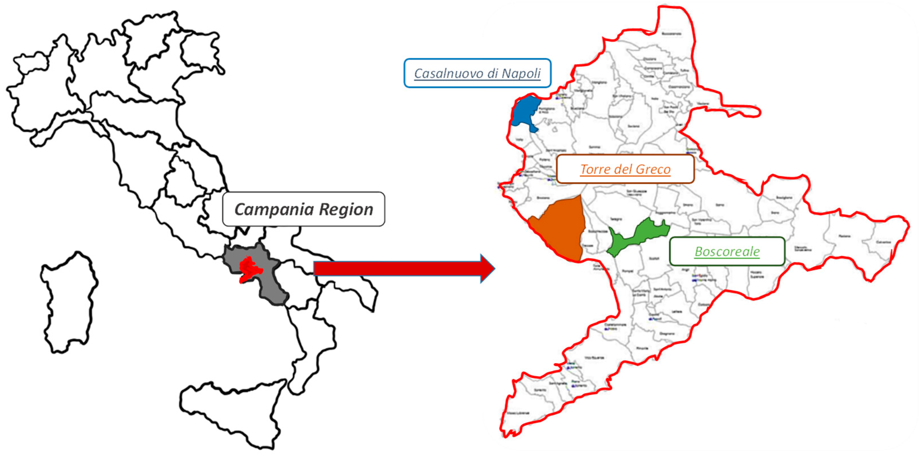
Figure 2.
Example of mean measured daily flow (µQ) pattern (-) and leakage flow pattern (-·-) for two DMAs with a different number of users.
Figure 2.
Example of mean measured daily flow (µQ) pattern (-) and leakage flow pattern (-·-) for two DMAs with a different number of users.
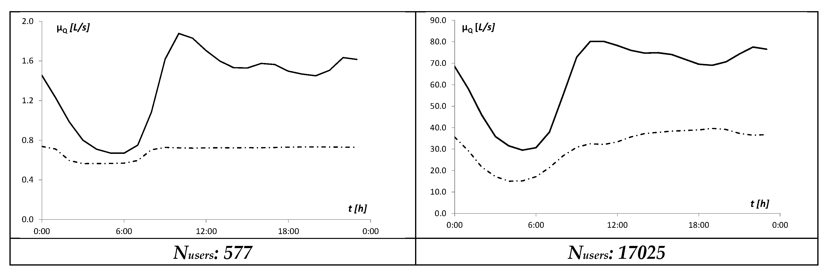
Figure 3.
Example of mean measured daily flow (µQ) pattern (-) and leakage flow pattern (-·-) for a DMA without PRV (702 users). Comparison of the flow pattern (-·-) with the constant leakages estimation (····).
Figure 3.
Example of mean measured daily flow (µQ) pattern (-) and leakage flow pattern (-·-) for a DMA without PRV (702 users). Comparison of the flow pattern (-·-) with the constant leakages estimation (····).
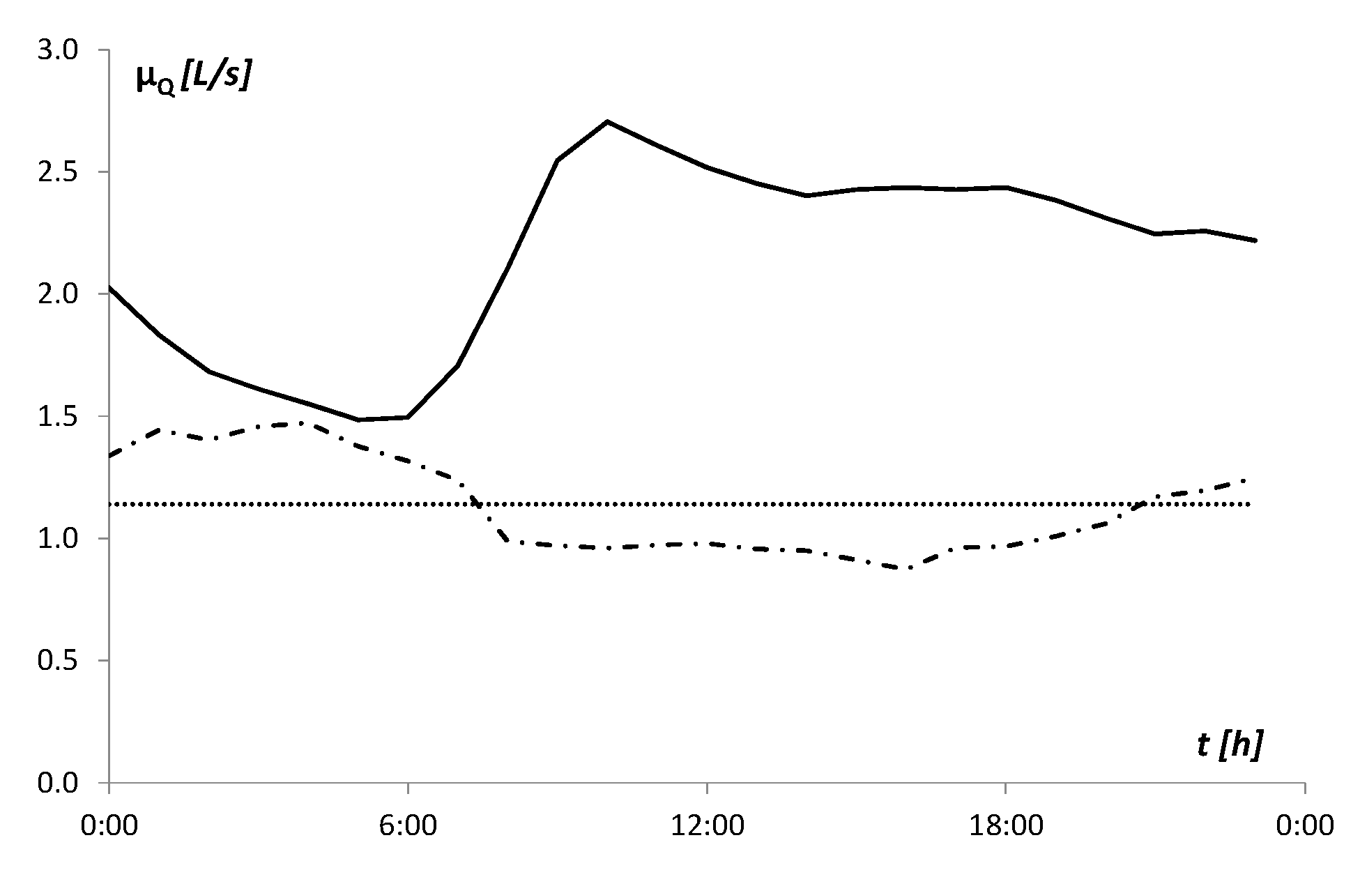
Figure 4.
Q-Q plots of the Cdmin for the different distribution considered and for ΔT =1h, at varying the users number.
Figure 4.
Q-Q plots of the Cdmin for the different distribution considered and for ΔT =1h, at varying the users number.
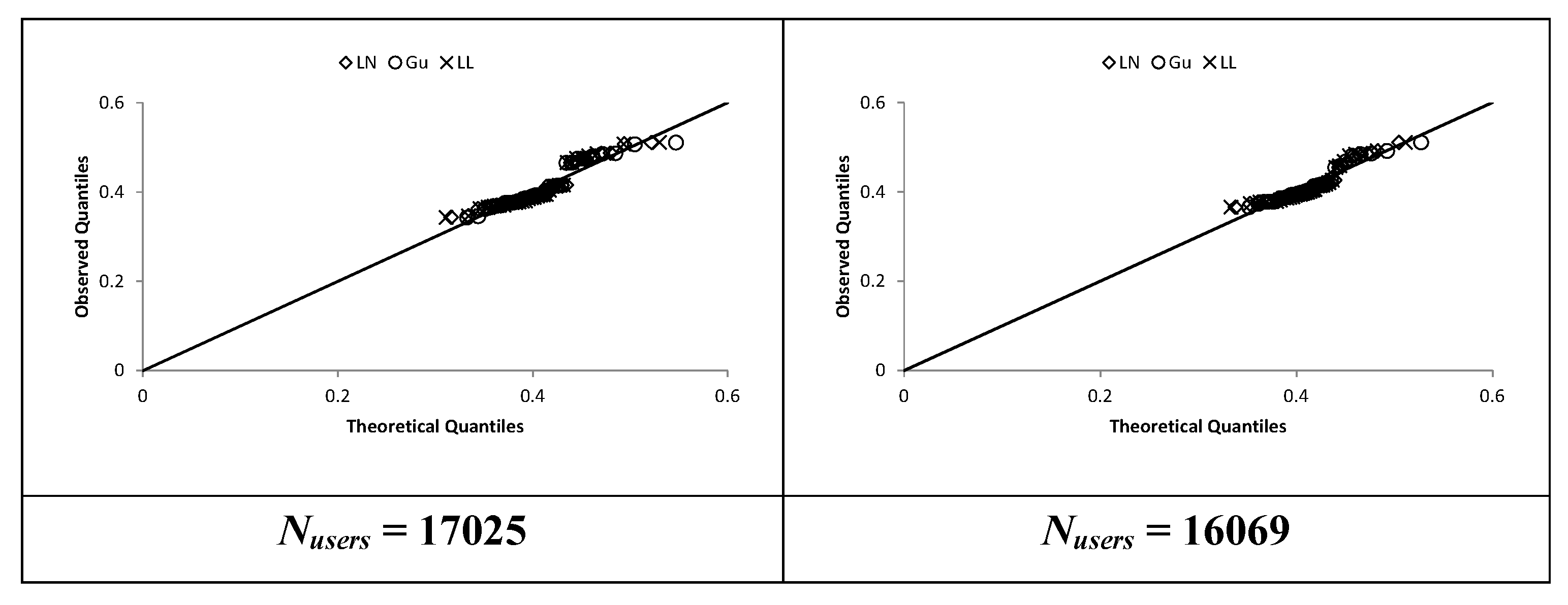
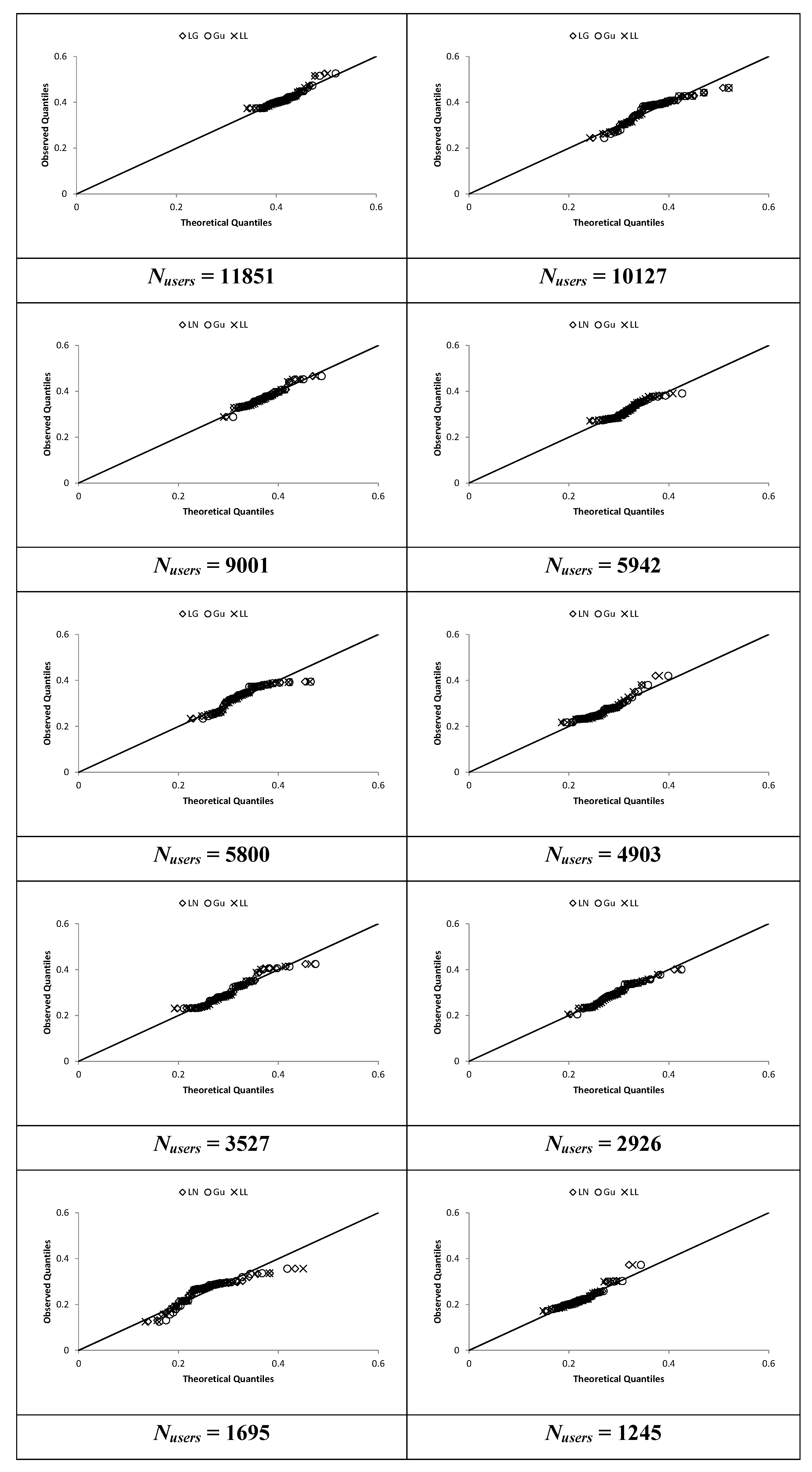
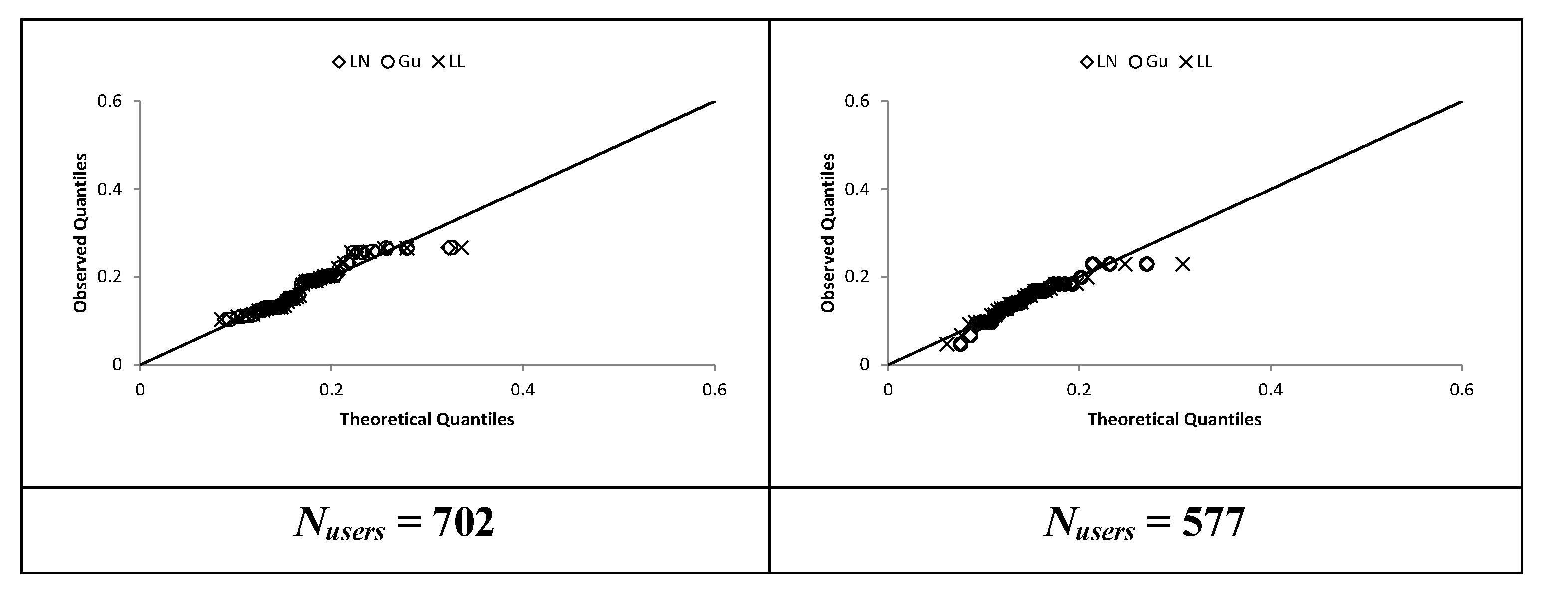
Figure 5.
KS test results for the analysed samples.
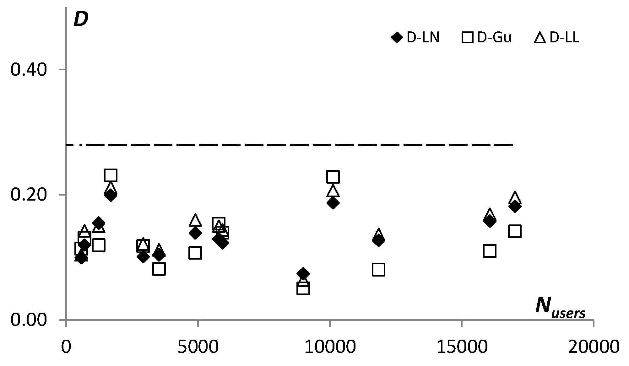
Figure 6.
DMA mean Cd minimum () at varying the number of users.
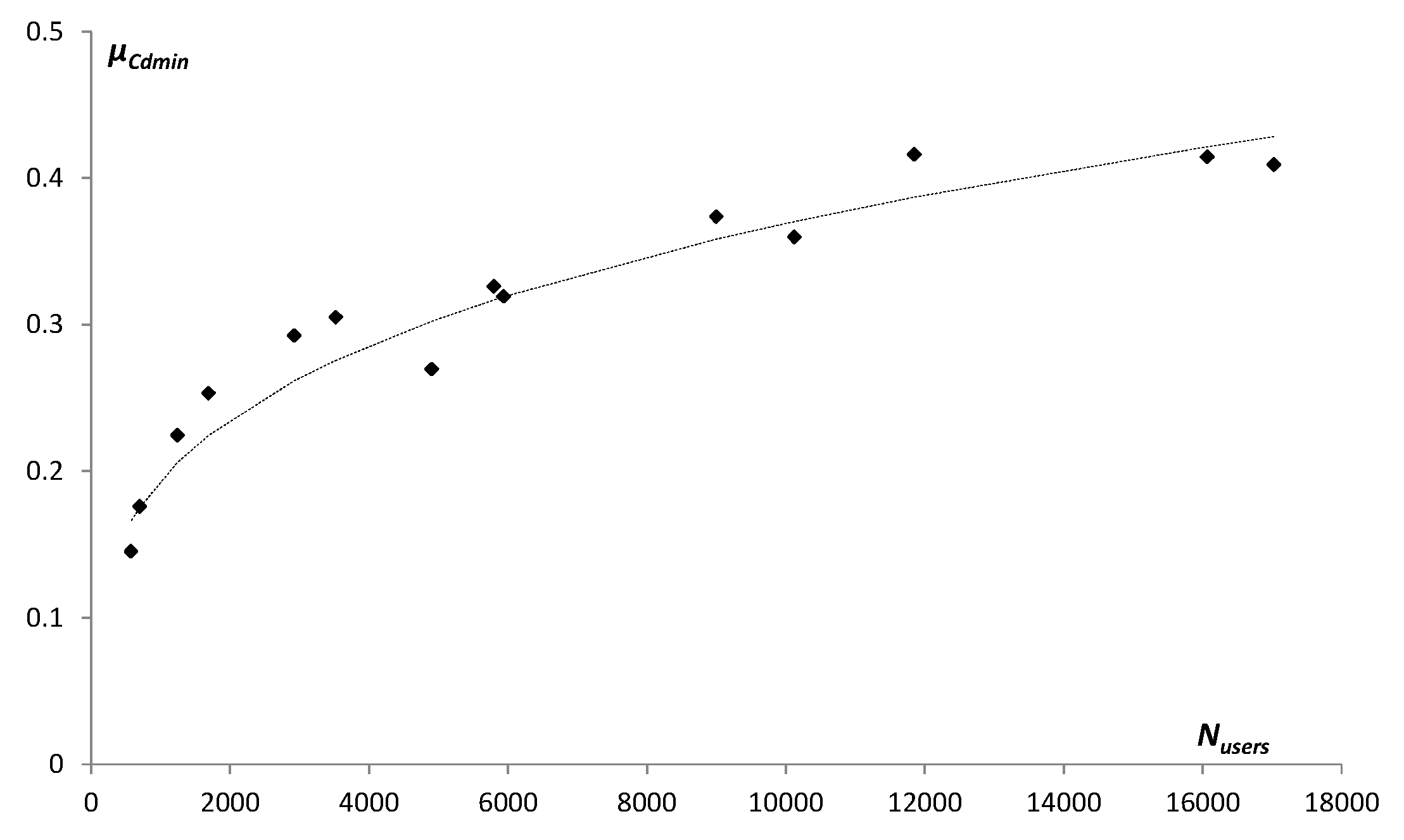
Figure 7.
CV of Cdmin at varying the number of users.
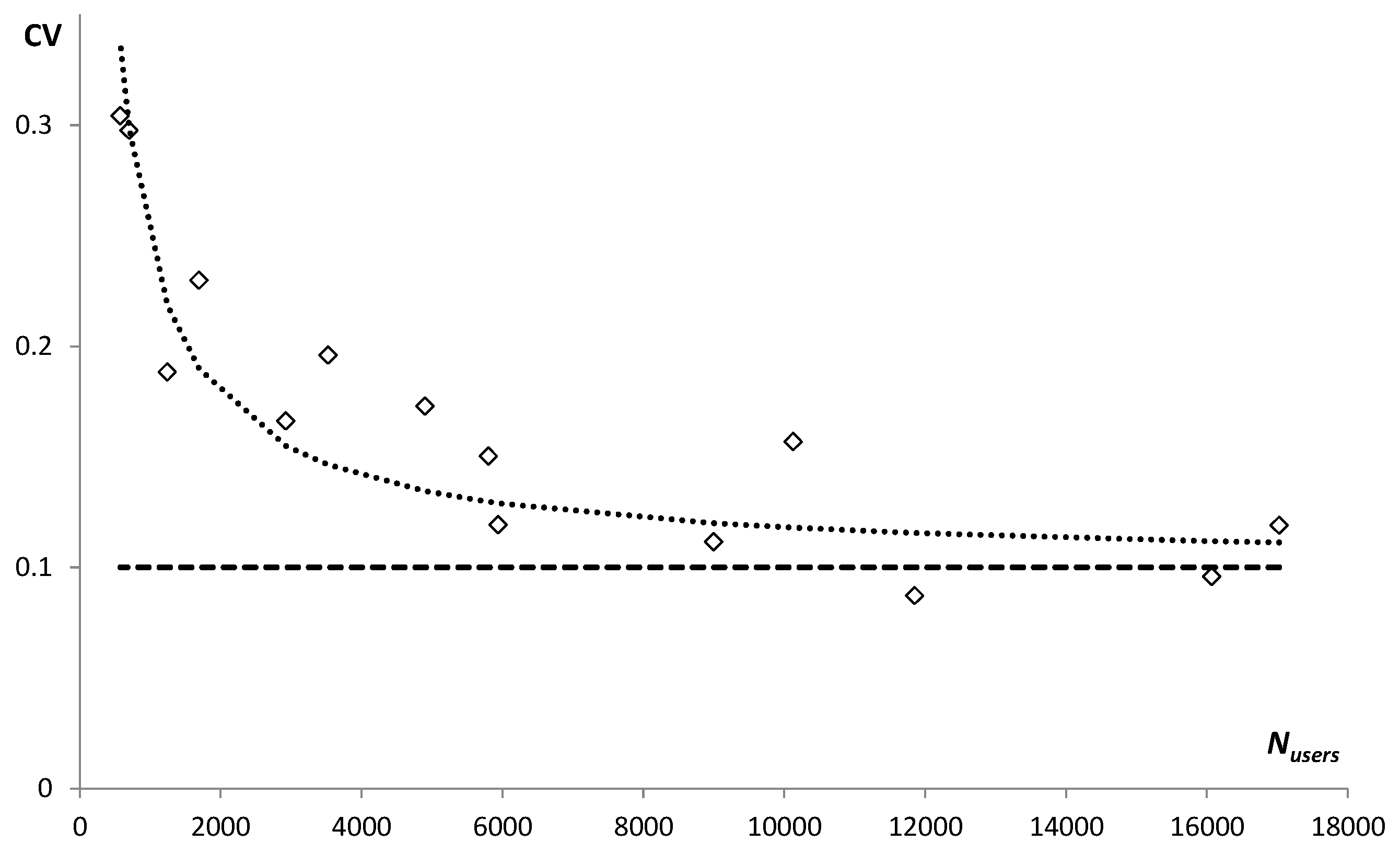
Figure 8.
Mean Cdmin variation with the number of users for predefined confidence interval estimated with the CDF of Gumbel distribution.
Figure 8.
Mean Cdmin variation with the number of users for predefined confidence interval estimated with the CDF of Gumbel distribution.
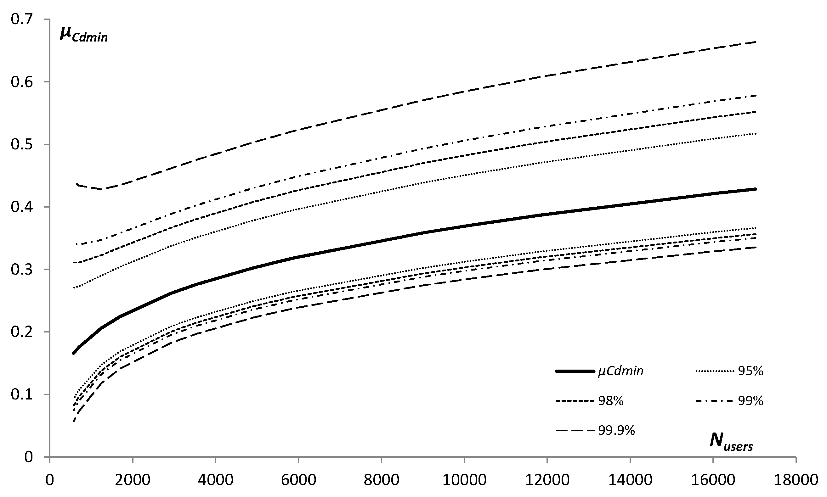
Figure 9.
Observed and estimated CDF for different users number.
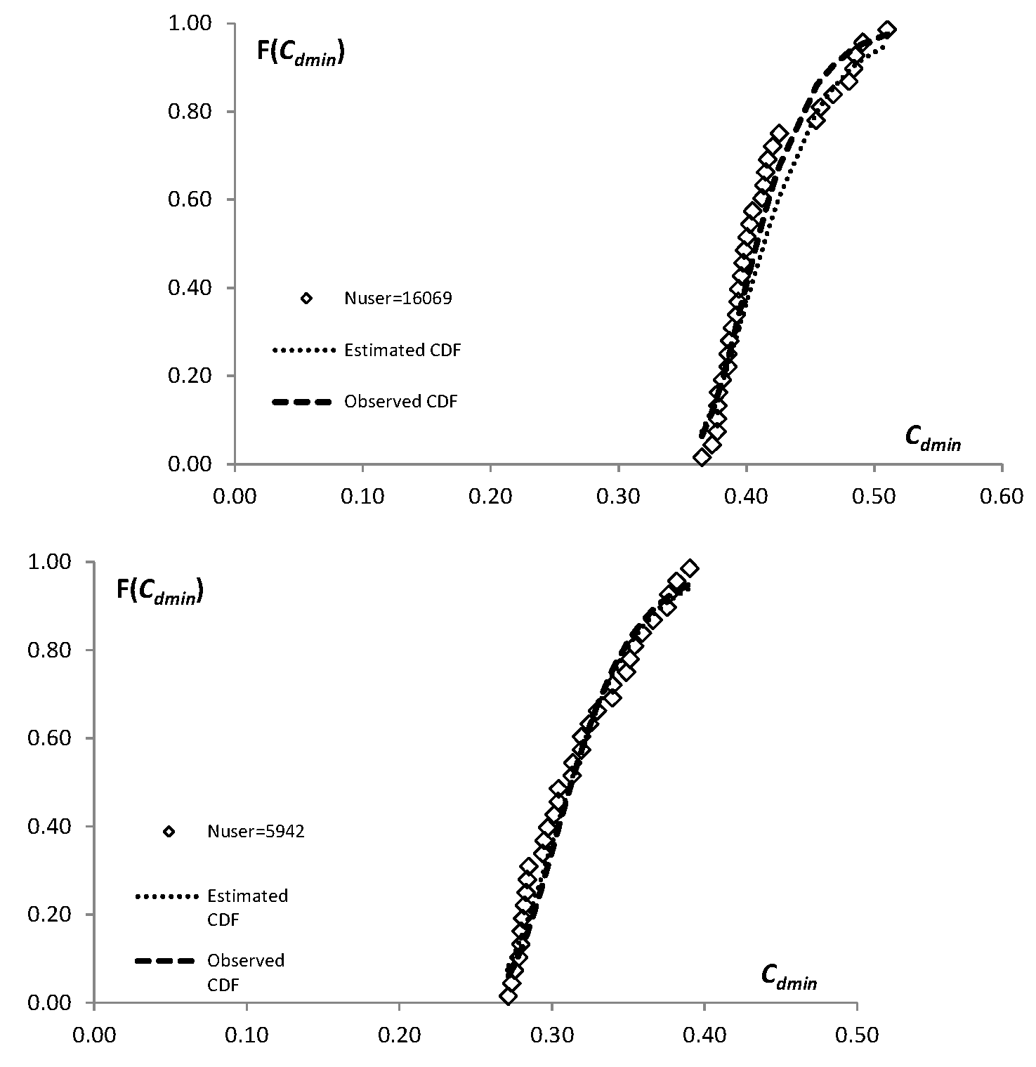

Table 2.
Statistics for the analysed samples and goodness of fit with D K-S.
| Nusers | Cdmin | Cdmin | DLN | DGu | DLL | D1% |
|---|---|---|---|---|---|---|
| 17025 | 0.409 | 0.049 | 0.181 | 0.141 | 0.195 | 0.280 |
| 16069 | 0.415 | 0.040 | 0.157 | 0.110 | 0.169 | 0.280 |
| 11851 | 0.416 | 0.036 | 0.126 | 0.080 | 0.136 | 0.280 |
| 10127 | 0.360 | 0.056 | 0.187 | 0.229 | 0.206 | 0.280 |
| 9001 | 0.374 | 0.042 | 0.073 | 0.050 | 0.063 | 0.303 |
| 5942 | 0.319 | 0.038 | 0.122 | 0.139 | 0.143 | 0.280 |
| 5800 | 0.326 | 0.049 | 0.129 | 0.153 | 0.149 | 0.280 |
| 4903 | 0.270 | 0.047 | 0.138 | 0.107 | 0.159 | 0.288 |
| 3527 | 0.305 | 0.060 | 0.103 | 0.081 | 0.111 | 0.280 |
| 2926 | 0.292 | 0.049 | 0.101 | 0.118 | 0.121 | 0.298 |
| 1695 | 0.253 | 0.058 | 0.199 | 0.231 | 0.211 | 0.280 |
| 1245 | 0.225 | 0.042 | 0.154 | 0.119 | 0.149 | 0.280 |
| 702 | 0.176 | 0.052 | 0.119 | 0.131 | 0.142 | 0.280 |
| 577 | 0.145 | 0.044 | 0.099 | 0.114 | 0.103 | 0.280 |
Disclaimer/Publisher’s Note: The statements, opinions and data contained in all publications are solely those of the individual author(s) and contributor(s) and not of MDPI and/or the editor(s). MDPI and/or the editor(s) disclaim responsibility for any injury to people or property resulting from any ideas, methods, instructions or products referred to in the content. |
© 2024 by the authors. Licensee MDPI, Basel, Switzerland. This article is an open access article distributed under the terms and conditions of the Creative Commons Attribution (CC BY) license (http://creativecommons.org/licenses/by/4.0/).
Copyright: This open access article is published under a Creative Commons CC BY 4.0 license, which permit the free download, distribution, and reuse, provided that the author and preprint are cited in any reuse.


