
Submitted:
12 November 2024
Posted:
13 November 2024
You are already at the latest version
Abstract
In this paper, we obtain new t-norms and t-conorms on some important subfamilies of the set of functions from [0,1] to [0,1]. In particular, we define these new operators on the subsets of the functions that are convex, normal, normal and convex, the functions taking only the values 0 or 1 and its subset of the functions whose support is a finite union of closed intervals. These t-norms and t-conorms are generalized to the type-2 fuzzy sets framework.
Keywords:
Function from [0
; 1] to [0
; 1]
; normal function
; convex function
; type-2 fuzzy set
; interval type-2 fuzzy set
; t-norm
; t-conorm
1. Introduction
When working with type-1 fuzzy sets (FSs), we may find that different agents assign different membership values to the same element. This disparity is inherent in the fact that different people may consider different meanings for the same words or different sensors may read the same data differently due to intrinsic errors in the measurements. More generally in fuzzy set theory every aspect is subject to the graduation of its membership including the degree of membership. To address this issue, L.A. Zadeh introduced type-2 fuzzy sets (T2FSs) as an extension of type-1 fuzzy sets (see [42,43]). A T2FS is determined by a membership function from the universe X to M, where M is the set of functions from [0,1] to [0,1]. T2FSs are more general than FSs and more suitable for modeling uncertainty, vagueness and/or imprecision in specific situations. This is a consequence of the fact that, in the context of FSs, the degree of membership of an element to a set is given by a value in the interval while in the case of T2FSs this degree of membership is a fuzzy set in (see for instance [24,28,29,37]).
Many T2FSs families have been also developed to cope with the lack of knowledge or uncertainty of the experts valuations. The authors recommend the thorough overview [3]. Computationally efficient methods have been developed to transfer this reality into applications (see for example [7,8,9,22,23,25]). A large number of them are devoted to the feasibility of type-2 fuzzy logic systems (T2FLSs). As a result of these computational simplifications, the first applications are now being implemented (see [6,21,30,35]).
In this paper we consider T2FSs with membership degrees in some families of the set of all functions from [0,1] to [0,1]. In particular, we will focus our attention in the next subsets of :
- C: set of convex functions of .
- N: set of normal functions of .
- L: set of both convex and normal functions of .
- K: functions of N, whose images are 0 or 1 (but not all 0).
- : functions of K whose support is a finite union of closed intervals. In the notation , c stands for close and F for finite.
Since the article of Bustince et al. [2], the interest in the set K has increased significantly (see for example [15,32]). In these works they show, among other things, theoretical and applied examples, about the advantage on the use of this set K. In particular, Ruiz-García et al. noted in [32] that it can be used to easily capture uncertainty without imposing unnecessary and unrealistic conditions on IVFSs, which can be extremely useful in intelligent systems.
The aim of this work is to define new triangular norms and triangular conorms in the aforementioned subsets of . Triangular norms (t-norms) were first introduced by Menger in [27] in the context of metric probabilistic spaces. Later, Schweizer and Sklar reformulated the definition of t-norms in [33,34] establishing the axioms now used to define them. A thorough study about t-norms is given in [19]. Fuzzy set theory is strongly related to order theory (see for instance [12]). Hence the usefulness of defining t-norms on bounded partially ordered sets also known as bounded posets (see [4,5]). Specifically, it is interesting to define t-norms on bounded lattices as Ray did in [31].
The study of t-norms and t-conorms over more complex types of fuzzy sets started with Gehrke et al. in [11], where they extended the definitions of t-norm and t-conorm to interval-valued fuzzy sets (IVFSs). Walker and Walker extended these axioms to T2FSs (see [37,38]) and presented two new families of binary operations on M. They also determined that, under certain conditions, they are t-norms and t-conorms on L. In [18], Hernández et al. obtained t-norms and t-conorms on L which are extensions of those established in [37,38]. Furthermore, the same authors defined in [17] new t-norms and t-conorms on L that are not obtained with the formulas given in previous works. Later, Wu et al. carried out a similar study introducing different new t-norms on this same set (see [39,40]). Neither t-norms nor t-conorms on C, N, K, or can be found in the literature. Even though K is not a lattice, in applications the operations on this set require less computational resources than those required on M.
The two main objectives of this paper are to analyze the operations presented in previous works (e.g. [17,18,37,38]) and to examine more general families of binary operations on M. More precisely, it is studied whether these operators satisfy the necessary axioms to be t-norms or t-conorms on M, C, N, L, K and .
The article is organized as follows. Section 2 establishes definitions, notations and properties required in the rest of this work. Section 2.1 is devoted to review some definitions and properties of FSs, IVFSs, T2FSs and IT2FSs. Section 2.2 provides some background on t-norms and t-conorms on such sets. Section 3 is the main part of the article. In Section 3.1 the operations considered in [16,18,37,38] are studied and we conclude that they are not t-norms or t-conorms on M, C, N, K and in general. Section 3.2 introduces new families of operations on the aforementioned subsets of M. More precisely, the properties of these operations are analyzed in order to determine if they are t-norms or t-conorms on M, C, N, L, K and . Finally, Section 4 summarizes the main results and states some conclusions.
2. Preliminaries
Throughout the paper, X will denote a non-empty set which will represent the universe of discourse. Additionally, ≤ will denote the usual order relation in the lattice of real numbers, and ∨ and ∧ the maximum and the minimum operators on the lattice , respectively.
2.1. Some Types of Fuzzy Sets and Operations
In this subsection, we present the definition of fuzzy set, interval-valued fuzzy set, type-2 fuzzy set and interval type-2 fuzzy set. Moreover, we establish some important properties and operations related to them.
Definition 1. ([41]) A type-1 fuzzy set (FS)Ais characterized by a membership function ,
where is the degree of membership of an element to the set A.
Definition 3. ([29]) A type-2 fuzzy set (T2FS)Ais characterized by a membership function:
where
M
is the set of all functions from the interval to itself,
That is, is a fuzzy set on the interval and also the degree of membership of an element to the set A. Therefore,
Next, let us present some subsets of M that we will consider in this work.
Definition 4.
A function is normal if,
and it is convex if for any , the inequality:
holds.
The set of all normal functions of M will be denoted by N, and the set of all convex functions of M will be denoted by C. Moreover, L will be the set of all normal and convex functions of M.
From now on, the notation for intervals between two slashes, , will refer to any non-empty interval (closed, open or half-open interval) in , and its characteristic function is defined as follows.
Definition 5.
([18]) Let , with , . The characteristic function of is , where:
Let us note that, the characteristic function of any interval in is an element of L.
Interval type-2 fuzzy sets are defined in [15] as follows:
Definition 6.([15]) A type-2 fuzzy set is said to be an interval type-2 fuzzy set (IT2FS) if for all ,
where is a constant function such that That is, for all and .
Note that the support of the function , in Definition 6, can be any subset of the interval and therefore it does not necessarily have to be a convex subset. Moreover, let us note that in [2,20,26] the authors include the constant function (with empty support), but in Definition 6 we exclude this function so as not to have two functions (the constant functions and ) to represent the lack of information (see [15]).
Let . Obviously, . Let us note that the support of any () is not empty, and it is the finite or infinite union of closed, open or half-open intervals. In addition, we consider the subset of , denoted by , constituted by the functions whose support is the finite union of closed intervals. Consequently .
The algebraic operations join, meet and complementation on M, given in the next definition, were determined from Zadeh’s Extension Principle ([41,42]).
Remark 1.
Note that ⊔ and ⊓ are idempotent, that is, and , for all . They also satisfy De Morgan’s laws respect to the given operation ¬ (see [37] for more details). Additionally, whenMis interpreted as the set of all linguistic labels of the “TRUTH” variable, then and (singletons of 0 and 1) represent the “completely false” and “completely true” labels, respectively.
does not have a lattice structure since it does not comply with the absorption law (see [14,37]). However, the operations ⊔ and ⊓ fulfill the properties required to each of them to define a partial order on M.
- The two partial orders ⊓ and ⊔ do not generally coincide.
- , and so , for all , that is, is the largest element of the partial order ⊑.
- , and then , for all , that is, is the smallest element of the partial order ⪯.
The following definition and theorems were given in previous papers in order to facilitate the operations on M:
Remark 3.
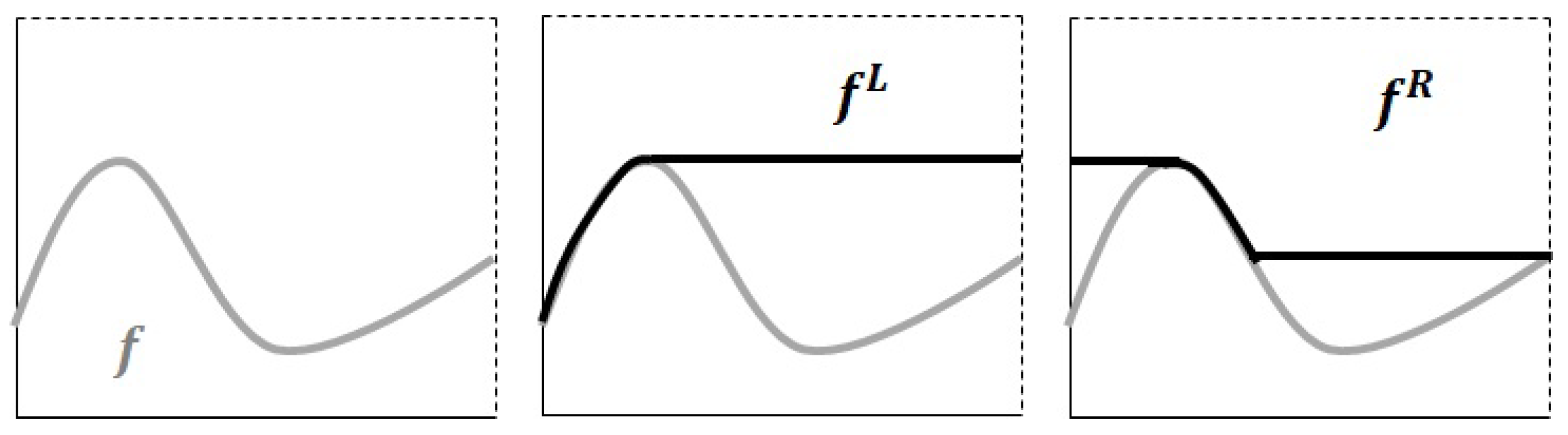
In [37], some of the properties of these new functions are obtained:
- and are monotonically increasing and decreasing, respectively (see for example Figure 2).
- and where ≤ is the usual pointwise order in the set of functions ( if and only if for all ).
- and .
- If we define and , the next assertion holds:
The following characterization was also shown in [37].
Note that the operations ∨ and ∧ have the usual meaning in the set of functions, that is, , and for all .
2.2. T-Norms and t-Conorms on Bounded Posets
In this section we recall some definitions and results about t-norms and t-conorms which will be used throughout Section 3. Remember that a t-norm on is a binary operation , which is commutative, associative, increasing on each argument, and with neutral element 1. Furthermore, a t-conorm on is a binary operation , commutative, associative, increasing on each argument and with neutral element 0. Similar definitions are applied to bounded posets (see [4,5]).
- for all (commutativity),
- for all (associativity),
- , for all (neutral element),
- Let such that , then (monotony).
- 3’.
- ,
are satisfied.
Example 1.
Here we present some important examples of t-norms and t-conorms on which will be used in the following:
- The minimum t-norm and the maximum t-conorm .
- The product t-norm and the probabilistic sum .
- The drastic t-norm and the drastic t-conorm:
In [36,37,38] it was shown that ⊓ and ⊔ are t-norm and t-conorm, respectively, on L, but no other study was done of these operations on other subsets of M. In [16,18] the two following families of binary operations on M were proposed. These operations are extensions of the ones given in [37,38].
In [18] it was shown that ▴ (▾) is a t-norm (t-conorm) on L given the order ⊑ (in this case ). Furthermore, the axioms of definitions 10 and 11 were studied on M, C and N, except for the monotony. We will study if these two operators are, respectively, t-norm and t-conorm on these and other subfamilies of M with both orders ⊑ and ⪯. In addition, we will define new operators that are indeed t-norms or t-conorms on some of these subsets.
The following theorem presents some properties of ▴ and ▾, that will allow us to prove some results in Section 3.
Theorem 3.([18]) For the operations ▴ and ▾ given in Definition 12, the following properties hold:
- ▴ and ▾ are commutative and associative in .
- , , and for all .
- , for all where .
- for all .
- for all .
-
and for all.
- Given , such that , then:
- , for all .
- For all such that and :
- If , then:
- ▴ and ▾ are closed onM,C,N, andL .
- ▴ and ▾ are t-norms and t-conorms, respectively, on the lattice .
3. T-norms and t-conorms on M, C, N, L, K and .
In this section, we will prove that, in general, the operations ▴ and ▾ are not t-norm and t-conorm on C, N, K, and respectively. Nevertheless, we will show that they are indeed t-norm and t-conorm in the particular case where and . Additionally we will perform a similar study, introducing new families of operators and analyzing for different orders if they are t-norms or t-conorms on M, C, N, L, K and .
3.1. The Operations ▴ and ▾ on M, C, N, K and .
The main purpose of this subsection is to show that ▴ and ▾ are not t-norms and t-conorms in general in any of the sets C, N, K and . In order to find the corresponding counterexamples, we need to go deeper into the structure of these families regarding the partial orders ⊑ and ⪯.
From the results in [37], it can be deduced that is the minimum and is the maximum element with respect to the partial order ⊑ on M and on C. Moreover, is the minimum and is the maximum regarding ⪯ on these same sets. It is also well known (see [15]) that and are, respectively, the minimum and the maximum of each one of the posets , , and . In the next result, we will show that these particular elements are the same in N.
Proposition 1.
The functions and , are, respectively, the minimum and the maximum ofN, respect to the partial orders ⊑ and ⪯.
Proof.
In [15] it was proved that is the maximum of and is the minimum of . Let us prove that , for all . It is known that , and that if , then . Hence:
and, according to Theorem 1, for all . The same procedure can be applied to show that is the maximum element of . □
In [18] it was proved that ▴ and ▾ are closed in C, N, and M. In the next result, we show that both operations are also closed in K and .
Proposition 2.
▴ and ▾ are binary operators in K
and .
Proof.
By definition, . We will only prove that ▴ is a closed operation on since the proof is analogous for ▾. If , it is clear that by the way we defined this operation. Consequently, we only need to show that whenever . In that case there exist and such that and . Fixing we have that:
which concludes this part of the proof.
Let us now show that ▴ is closed on (the proof for ▾ is analogous). Given , we only need to prove that . Since ▴ is closed on K, this is equivalent to state that is a union of closed intervals. In fact, as and for some finite , let us see that:
First, let us take an arbitrary . In this case:
The only possibility here is the existance of and such that . That is, there exist and with and . Consequently, and making use of the monotony of , we have that and hence:
Finally, let us consider for some . Since is a continuous function, there exist and with . Taking this into account, and thus, . Consequently, and equation (1) holds. Therefore, is the union of closed intervals and . □
Note that Theorem 3 establishes that the two operations satisfy the axioms 1 and 2 of t-norm and t-conorm in M, and also establishes that the operation ▴ satisfies axiom 3 on the poset and ▾ satisfies axiom 3’ on . Nevertheless, in general, they are not t-norms or t-conorms in M, N, K and respect to each partial order. Corollary 1, established in [15], will help us to reach this result.
Corollary 1.([15]) Let . And let , , , . Then,
- if and only if , , and , for all .
- if and only if , , and , for all .
Proposition 3.
▴ and ▾, in general, are neither t-norm nor t-conorm onM,N,Kand .
Proof.
It is enough to find the appropriate counterexamples where the operations are not increasing with respect to any of the two partial orders. In that case, t-norm (t-conorm) axiom 4 fails. Since , we only need to find these counterexamples in . Let , where
As a consequence of Corollary 1, and . Let us consider ▴, where for each we have , and . In this case,
and
By Corollary 1 we conclude that and . Therefore, ▴ is not always increasing on the bounded posets , , , , and and, consequently, on and .
Analogously, it is easy to prove that the operator ▾, where and for each , is not increasing with respect to any of the aforementioned partial orders. The same functions f and g defined above can be used. In this case:
Once again, using Corollary 1 we can check that and so the monotony of this operator on the posets of interest does not hold. □
A similar result to the previous one can be obtained for the set C.
Proposition 4.
▴ and ▾, in general, are neither t-norm nor t-conorm on or .
Proof.
First, we define:
It is easy to check that . Moreover, by Theorem 1 we have that since . However, if we set to define ▴ as in Definition 12 we can show that . With this purpose, let us prove that:
for . Since:
then inequality (2) holds. As a consequence of this and by means of Theorem 1 we get to the result. With this discussion, we have proven that ▴ is not always monotonically increasing in with respect to the order ⊑. Therefore, ▴ is neither t-norm nor t-conorm in .
Let us now show that ▾ is not monotonically increasing either, when we take and in its definition. Note that by Theorem 1 and that:
Thus we can state that:
By Theorem 1, and ▾ is neither t-norm nor t-conorm on C with respect to the order ⊑.
Let us now consider the order ⪯. Since , we have that and that:
Hence:
As a consequence, and ▴ is neither t-norm nor t-conorm on C with respect to the order ⪯. Moreover, it is clear that because the inequality holds. However:
Once again, we can make use of Theorem 1 and the inequality:
to show that . Therefore, ▾ is neither t-norm nor t-conorm on C with respect to the order ⪯. □
Remark 4.
It should be noted that in the particular cases of ▴ and ▾, with , these operators are t-norm and t-conorm onC, respectively, respect to both partial orders ⊑ and ⪯. See [37] and [18] for more details. However, in Proposition 4, we have shown that, generally, neither ▴ nor ▾ are monotonically increasing onCwith respect to any of the partial orders.
In spite of the previous results, there are particular cases in which ▴ and ▾ are t-norm and t-conorm, respectively, on the particular subsets of M that we are studying. We will show one of these cases.
Proposition 5.
⊓ (⊔) is a t-norm (t-conorm) onM,C,N,Kand respect to the partial order ⊑ (⪯).
Proof.
In [37] it was established that ⊓ and ⊔ are commutative and associative. Moreover, due to Theorem 3 and Proposition 2, we know that these functions are closed on M, C, N, K and . Again, by Theorem 3 we have that the neutral element for ⊓ is and for ⊔ is .
Let us check the monotony of ⊓ (⊔) respect to the partial order ⊑ (⪯). Let , with . Let us recall that if and only if . As ⊓ is commutative, associative and idempotent:
Thus, ⊓ is increasing in each argument on . Similarly, we can prove that ⊔ is increasing on .
As a consequence, since and , we have that ⊓ (⊔) is a t-norm (t-conorm) on M, C, N, K and , respect to the partial order ⊑ (⪯). □
Remark 5.
Note that () is the absorbent element of ⊓ (⊔) onN(see Theorem 3). Nevertheless, when working onC(orM) the constant function0is the absorbent element for both operators.
3.2. The Operations ⊥ and ⊤ on M, C, N, L, K and .
• In this subsection, two new operations, ⊥ and ⊤, will be introduced. It will be proven that ⊥ is a t-norm respect to the partial order ⊑ and ⊤ is a t-conorm respect to ⪯ on N, K and . In addition, we will show that ⊥ is a t-norm and ⊤ is a t-conorm on the lattice . Nevertheless, we will prove that there exist counterexamples where ⊥ (⊤) is not t-norm (t-conorm) on C (and consequently, on M) since, in this case, ⊥ is equivalent to ▴ and ⊤ is equivalent to ▾.
Definition 13.
Let , and ▴, ▾ the operations given in Definition 12. We define the following operations:
Remark 6.
In Definition 13 the minimum t-norm ∧ is used. However, when we work onN, all the results obtained are also fulfilled when we employ any other t-norm ⊼ on . This fact is easy to check. When , then for all either or . Since all t-norms are equivalent when one of the arguments takes the value 1, then and it does not matter which t-norm we use to define ⊥ or ⊤.
- ⊥ and ⊤ are equivalent to ▴ and ▾, respectively, on . If , then and (see [37]). Moreover since and for all , we can state that , on . Consequently, Proposition 4 provides counterexamples where ⊥ and ⊤ are neither t-norm nor t-conorm with respect to either order ⊑ or ⪯ onC, and therefore onM .
- Since and as a consequence of the previous point, ⊥ and ⊤ are also equivalent to ▴ and ▾, respectively, on . It was proven in [18] that ▴ (▾) is t-norm (t-conorm) on (L, ⊑, , ) so ⊥ (⊤) is also t-norm (t-conorm).
-
If or we can find examples where and . Let us consider the function:We have that , , but , and . Consequently, ⊥ and ⊤ are not equivalent in general to ▴ and ▾ onN,Kor .
The following proposition establishes that ⊥ (⊤) satisfy the axioms 1, 2 and 3 (1,2 and 3´) of t-norm (t-conorm) on M.
Proposition 6.
The operations ⊥ and ⊤ are commutative and associative onM. Moreover, and for all .
Proof.
The operations ⊥ and ⊤ are commutative and associative since ▴ and ▾ are commutative and associative (see Theorem 3). In addition, and by definition. □
Remark 7.
The boundary conditions of ⊥ and ⊤ in Definition 13, guarantee the fulfillment of the axioms 3 and 3’, respectively. In fact, if they had not been added, these axioms would not always have to be fulfilled.
To prove this fact, let us suppose that we do not include the boundary conditions. If , we have that would not be the neutral element of the operation ⊥, since:
Moreover, would not be the neutral element of ⊤, since:
In order to analyze if these new operations are closed on N, K and , we previously present some properties.
Proposition 7.
i) If , then .
- ii)
- for all .
- iii)
- for all .
Proof.
i) It is known (see [37]) that a function is convex if and only if it is the minimum of two functions, one of them increasing and the other one decreasing. Since is increasing and is decreasing, for all . Moreover, and:
since . Therefore, and . Consequently, .
- ii)
- For all , we have that . Hence:and the desired property is proven.
- iii)
- The proof is analogous to the previous one.
□
Proposition 8.
The following properties hold:
- i)
- ii)
Consequently, operations ⊥ and ⊤ are closed onN,CandL
.
Proof.
i) Given that both and are in for all , and that the operations ▴ y ▾ are closed on C (see Theorem 3) the property is directly deduced.
- ii)
- By Proposition 7 i), if , then and . Once again, by Theorem 3, we know that ▴ and ▾ are closed operations on L so the result is verified.
The fact that ⊥ and ⊤ are closed on N, C and L is a direct consequence of the previous properties. □
In the following proposition we state that the defined operators are binary operations on K and .
Proposition 9.
⊥ and ⊤ are closed on and on .
Proof.
Let us first note that if with and , then:
Given , for all we have and for all we have . Consequently, will be closed if , and half-open otherwise. Similarly, will be closed if , and half-open otherwise. In particular, if , we have that and then:
That is, they have closed supports.
The next step is to see that if , then:
Moreover, if or the interval will be closed in such endpoint. Otherwise, it will be open. In particular, if , we have will have:
Since , we know that , and . Therefore:
We can be sure that because, for each , there exists such that . Consequently:
and so it is clear that This proves the assertion (3).
In addition, if , clearly and . Thus, is closed in . Otherwise, if , then , and . Therefore, is open in . A similar analysis can be done in the other endpoint . Hence, if or , then will be closed in the corresponding endpoint.
Now we can check that the operations ⊥ and ⊤ are closed on and on . Let . If , then and , as shown above. Moreover, by Theorem 3, we have:
Otherwise, if or , the operation is trivially closed on since and .
We can prove that ⊤ is a binary operation on in a similar way.
Finally, let . If , then and . Using Theorem 3 again, we can state that . Otherwise, and .
The fact that ⊤ is closed on K can be shown similarly. □
The following proposition presents the absorbent elements of ⊥ and ⊤ in N. Since these elements belong to the subsets L, K and , they will also be absorbent elements of these sets.
Proposition 10.
If , then and .
Proof.
According to Definition 13, we have and . Moreover, by Theorem 3:
□
Our next goal is to study the monotony of ⊥ and ⊤ on N and hence on K and . However, let us previously analyze the monotony of these operations without considering the boundary conditions.
Proposition 11.
Let , with . Then:
- .
Let , with . Then:
- .
Proof.
We will only prove the first inequality since the second one can be shown analogously. Let , with . First note that, according to Theorem 3 and and Theorem 7 ii):
In a similar way:
Since , by Lemma 1 in [15] we have that and . With this fact and Theorem 3:
and
Moreover, if , then , (see Proposition 8). Hence, from Theorem 2:
and the monotony on is proved. □
Proposition 12.
The following properties hold:
- i)
- The operation ⊥ is increasing in each argument on , and .
- ii)
- The operation ⊤ is increasing in each argument, on , and .
Proof.
Let us prove that the operation ⊥ is increasing respect to the partial order ⊑. Let , such that . We have to distinguish four cases:
- If all functions and h are different from , by Proposition 11 we have:
- If , since and g is the maximum, then . Thus, .
- If , then
-
Finally, let us see the case in which and . Here, and . As a consequence, it is sufficient to prove that:As , from Proposition 11 and Theorem 3:Let us check that . By Theorem 1 the inequality:must hold. According to Proposition 7, this inequality is equivalent towhich trivially holds. Then, ⊥ is increasing on each argument on . Consequently, it is also increasing in each argument on and .
The proof is similar when it comes to showing that ⊤ is increasing on , and . □
Corollary 2.
The following statements hold:
- i)
- ⊥ is a t-norm on , and , with neutral element and absorbent element .
- ii)
- ⊤ is a t-conorm on , and , with neutral element and absorbent element .
Proof.
All the necessary properties for ⊥ to be a t-norm and for ⊤ to be a t-conorm in the above mentioned posets have been proved in the previous results of this subsection. □
The following example shows that ⊥ does not satisfy the monotony respect to the partial order ⪯ on M, N, K and . In the same way, it shows that ⊤ does not satisfy the axiom of monotony respect to ⊑ on these sets.
Example 2.
Let us consider the following functions on :
and let us take . In this case, . Since:
we have that (see Corollary 1).
Furthermore, . If we fix , the next identity holds:
and, by Corollary 1:
Therefore, neither ⊥ nor ⊤ are increasing in each argument respect to the corresponding orders.
4. Concluding Remarks
In this paper, we have introduced some new binary operations on M: ⊥ and ⊤. We have analyzed when the considered operations satisfy the required axioms for them to be t-norms or t-conorms on M, C, N, L, K and with respect to the two most commonly used partial orders on M. Let us present a list that contains the main results obtained:
- The operator ▴, with and , is neither increasing with respect to ⊑ nor with respect to ⪯ on M, N, K and .
- The operator ▾, with and is neither increasing with respect to ⊑ nor with respect to ⪯ on M, N, K and .
- The operator is t-norm on M, C, N, K and with respect to ⊑.
- The operator is t-conorm on M, C, N, K and with respect to ⪯.
- In general, the operators ▴, ▾, ⊥ and ⊤ are neither t-norm nor t-conorm, on C with respect to either ⊑ and ⪯.
- The operator ⊥ is t-norm on N, L, K and with respect to the order ⊑. Moreover, on C.
- The operator ⊤ is t-conorm on N, L, K and with respect to the order ⪯. Moreover, on C.
We are currently conducting a study of different new operations, which could be t-norms or t-conorms on some of the families that we are considering. We hope to present these results soon. Moreover, we will study other structures in type-2 fuzzy sets. In particular, aggregations, contradictions or similarities on M, C, N, K and .
Author Contributions
Conceptualization, P.H., F.T., S.C. and C.T; methodology, P.H., F.T., S.C., C.T. and J.E; validation, S.C., C.T. and J.E.; formal analysis, P.H., F.T., S.C., C.T. and J.E; investigation, P.H., F.T., S.C., C.T. and J.E; writing—original draft preparation, P.H., S.C. and C.T. ; writing—review and editing, P.H., F.T., S.C., C.T. and J.E ; supervision, S.C., C.T. and J.E; project administration, S.C., C.T. and J.E; funding acquisition, S.C., C.T. and J.E. All authors have read and agreed to the published version of the manuscript.
Funding
This research was funded by the Spanish Ministerio de Ciencia e Innovación/AEI/EU FEDER Funds, grant number PID2021-122905NB-C22, the Vicerrectoría de Investigación y Doctorados de la Universidad San Sebastián, Chile–USS–FIN–24–PASI–11 and the “Asociación de Amigos” of the University of Navarra.
Data Availability Statement
No new data were created or analyzed in this study. Data sharing is not applicable to this article.
Acknowledgments
This paper has been partially supported by the Spanish Ministerio de Ciencia e Innovación/AEI/EU FEDER Funds (grant PID2021-122905NB-C22). Pablo Hernández thanks the Vicerrectoría de Investigación y Doctorados de la Universidad San Sebastián, Chile–USS–FIN–24–PASI–11. Francisco Javier Talavera thanks the support of the “Asociación de Amigos” of the University of Navarra.
Conflicts of Interest
The authors declare no conflicts of interest.
Abbreviations
The following abbreviations are used in this manuscript:
| FS | Fuzzy set |
| IVFS | Interval-Valued Fuzzy Set |
| T2FS | Type-2 Fuzzy Set |
| IT2FS | Interval Type-2 Fuzzy Set |
| T2FLS | Type-2 Fuzzy Logic System |
References
- H. Bustince, E. H. Bustince, E. Barrenechea and M. Pagola, “Generation of interval-valued fuzzy and Atanassov’s intuitionistic fuzzy connectives from fuzzy connectives and from Kα operators. Laws for conjunctions and disjunctions. Amplitude”, Internat. J. Intell. Syst., vol. 23, pp. 680–714, 2008. [CrossRef]
- H. Bustince, J. H. Bustince, J. Fernandez, H. Hagras, F. Herrera, M. Pagola and E. Barrenechea, “Interval Type-2 Fuzzy Sets are Generalization of Interval-Valued Fuzzy Sets: Toward a Wider View on Their Relationship”, IEEE Trans. Fuzzy Syst., vol. 23, no. 5, pp. 1876–1882, 2015. [CrossRef]
- H. Bustince, E. H. Bustince, E. Barrenechea, M. Pagola, J. Fernandez, Z. Xu, B. Bedregal, J. Montero, H. hagras, F. Herrera and B. De Baets, B. (2015). A historical account of types of fuzzy sets and their relationships. IEEE Trans. Fuzzy Syst. 2015; 1. [Google Scholar] [CrossRef]
- De Baets, B. , Mesiar, R.: Triangular norms on product lattices. Fuzzy Sets and Systems, 104, 61–75 (1999). [CrossRef]
- De Cooman, G. , Kerre, E.: Order norms on bounded partially ordered sets. Journal Fuzzy Mathematics, 2, 281–310 (1994).
- S. Coupland, M. S. Coupland, M. Gongora, R. John, and K. Wills, “A comparative study of fuzzy logic controllers for autonomous robots”, in Proc. IPMU, Paris, France, Jul. 2006, pp. 1332–1339.
- S. Coupland and R. John, “A fast geometric method for defuzzification of type-2 fuzzy sets”, IEEE Trans. Fuzzy Syst., vol. 16, no. 4, pp. 929–941, 2008. [CrossRef]
- S. Coupland and R. John, “Fuzzy logic and computational geometry”, in Proceedings of RASC 2004, Nottingham, England, 2004, pp. 3–8.
- S. Coupland and R. John, “Geometric type-1 and type-2 fuzzy logic systems”, IEEE Trans. Fuzzy Syst., vol. 15, no.1, pp.3–15, 2007. [CrossRef]
- Z. Gera and J. Dombi, “Exact calculations of extended logical operations on fuzzy truth values”, Fuzzy Sets Syst., vol. 159, no. 11, pp. 1309–1326, 2008. [CrossRef]
- Gehrke, M. , Walker, C., Walker, E.: Some comments on interval-valued fuzzy sets. Internat. J. Intell. Systems, 11, 751–759 (1996).
- J. Goguen, “L-fuzzy sets”, J. Math. Anal. Appli., vol. 18, no. 1, pp. 623–668, 1967.
- J. Harding, C. J. Harding, C. Walker and E. Walker, “Convex normal functions revisited”, Fuzzy Sets Syst., vol. 161, pp. 1343–1349, 2010. [CrossRef]
- J. Harding, C. J. Harding, C. Walker and E. Walker, “Lattices of convex normal functions”, Fuzzy Sets Syst., vol. 159, pp. 1061–1071, 2008. [CrossRef]
- Hernández, P. , Cubillo, S., Torres-Blanc, C.: A Complementary Study on General Interval Type-2 Fuzzy Sets. IEEE Transactions on Fuzzy Systems, 30 (11), 5034–5043 (2022). [CrossRef]
- P. Hernández, S. P. Hernández, S. Cubillo and C. Torres-Blanc, “Negations on type-2 fuzzy sets”, Fuzzy Sets Syst., vol. 252, pp. 111–124, 2014. [CrossRef]
- Hernández, P. , Cubillo, S., Torres-Blanc, C.: Nuevas operaciones binarias sobre los conjuntos borrosos de tipo 2, en: Actas Multiconferencia CAEPIA 2013, 1250–1259 (2013).
- P. Hernández, S. P. Hernández, S. Cubillo and C. Torres-Blanc, “On t-norms on type-2 fuzzy sets”, IEEE Trans. Fuzzy Syst., vol. 23, no. 4, pp. 1155–1163, 2015. [CrossRef]
- Klement, P. , Mesiar, R., Pap, E.: Triangular Norms. Kluwer Academic Publishers, Dordrecht, The Netherlands (2000).
- Q. Liang and J.M. Mendel, “Interval type-2 fuzzy logic systems: theory and design”, IEEE Trans. Fuzzy Syst., vol. 8, no. 5, pp. 535–550, 2000. [CrossRef]
- O. Linda and M. Manic, “General type-2 fuzzy C-means algorithm for uncertain fuzzy clustering”, IEEE Trans. Fuzzy Syst., vol. 20, no. 5, pp. 883–897, 2012. [CrossRef]
- O. Linda and M. Manic, “Monotone centroid flow algorithm for type reduction of general type-2 fuzzy sets”, IEEE Trans. Fuzzy Syst., vol. 20, no. 5, pp. 805–819, 2012. [CrossRef]
- F. Liu, “An efficient centroid type-reduction strategy for general type-2 fuzzy logic system”, Inf. Sci., vol. 178, pp. 2224–2236, 2008. [CrossRef]
- J. Mendel and R. Jhon, “Type-2 fuzzy sets made Simple”, IEEE Trans. Fuzzy Syst., vol. 10, no. 2, pp. 117–127, 2002. [CrossRef]
- J. Mendel, F. J. Mendel, F. Liu, and D. Zhai, “α-plane representation for type-2 fuzzy sets: theory and applications”, IEEE Trans. Fuzzy Syst., vol. 17, no. 5, pp. 1189–1207, Oct. 2009. [CrossRef]
- J. M. Mendel, R. I. J. M. Mendel, R. I. John and F. Liu, “Interval type-2 fuzzy logic systems made simple”, IEEE Trans. Fuzzy Syst., vol. 14, no. 6, pp. 808–821, 2006. [CrossRef]
- Menger, K. : Statical metrics. Proc. Nat. Acad. Sci. U.S.A., 37, 535-537 (1942).
- M. Mizumoto and K. Tanaka, “Fuzzy sets of type-2 under algebraic product and algebraic sum”, Fuzzy Sets Syst., vol. 5, pp. 277–290, 1981. [CrossRef]
- M. Mizumoto and K. Tanaka, “Some properties of fuzzy sets of type-2”, Inf. Control, vol. 31, pp. 312–340, 1976.
- A. Niewiadomski, “On finity, countability, cardinalities, and cylindric extensions of type-2 fuzzy sets in linguistic summarization of databases”, IEEE Trans. Fuzzy Syst., vol. 18, no. 3, pp. 532–545, 2010. [CrossRef]
- S. Ray, “Representation of a Boolean algebra by its triangular norms”, Mathware and Soft Computing, vol. 4, pp. 63–68, 1997.
- G. Ruiz-García, H. G. Ruiz-García, H. Hagras, I. Rojas and H. Pomares, “Towards a Framework for Singleton General Forms of Interval Type-2 Fuzzy Systems”, Lecture Notes in Computer Science, pp. 3–26, 2017. [CrossRef]
- Schweizer, B. , Sklar, A.: Associative functions and statistical triangle inequalities. Publ. Math., 8, 169–186 (1961).
- Schweizer, B. , Sklar, A.: Statistical metric spaces. Pacific J. Math., 10, 313–334 (1960).
- C. Wagner and H. Hagras, “Toward general type-2 fuzzy logic systems based on zSlices”, IEEE Trans. Fuzzy Syst., vol. 18, no. 4, pp. 637–660, Aug. 2010. [CrossRef]
- C. Walker and E. Walker, “Some general comments on fuzzy sets of type-2”, Internat. J. Intell. Syst., vol. 24, pp. 62–75, 2009.
- C. Walker and E. Walker, “The algebra of fuzzy truth values”, Fuzzy Sets Syst., vol. 149, pp. 309–347, 2005.
- Walker, C. , Walker, E.: T-norms for type-2 fuzzy sets. In: Proc. Internat. Conf. on Fuzzy Systems IEEE 2006, pp. 1235–1239, –21, Vancouver (Canadá) (2006). 16 July. [CrossRef]
- X. Wu and G. Chen, “Answering an open problem on t -norms for type-2 fuzzy sets”, Inform. Sci., vol. 522, pp. 124–133, 2020. [CrossRef]
- X.Wu, G. X.Wu, G.Chen and L.Wang, “On union and intersection of type-2 fuzzy sets not expressible by the sup-t-norm extension principle”, Fuzzy Sets Syst., vol. 441, pp. 241–261 (2022). [CrossRef]
- L. Zadeh, “Fuzzy sets”, Inf. Control, vol. 20, pp. 301–312, 1965.
- L. Zadeh, “The concept of a linguistic variable and its application to approximate reasoning-I”, Inf. Sci., vol. 8, no. 3, pp. 199–249, 1975. [CrossRef]
- L. Zadeh, “The concept of a linguistic variable and its application to approximate reasoning-II”, Inf. Sci., vol. 8, no. 4, pp. 301–357, 1975. [CrossRef]
Figure 1.
([16], Fig. 5) Example for the operations ⊔, ⊓, and ¬.
Figure 1.
([16], Fig. 5) Example for the operations ⊔, ⊓, and ¬.
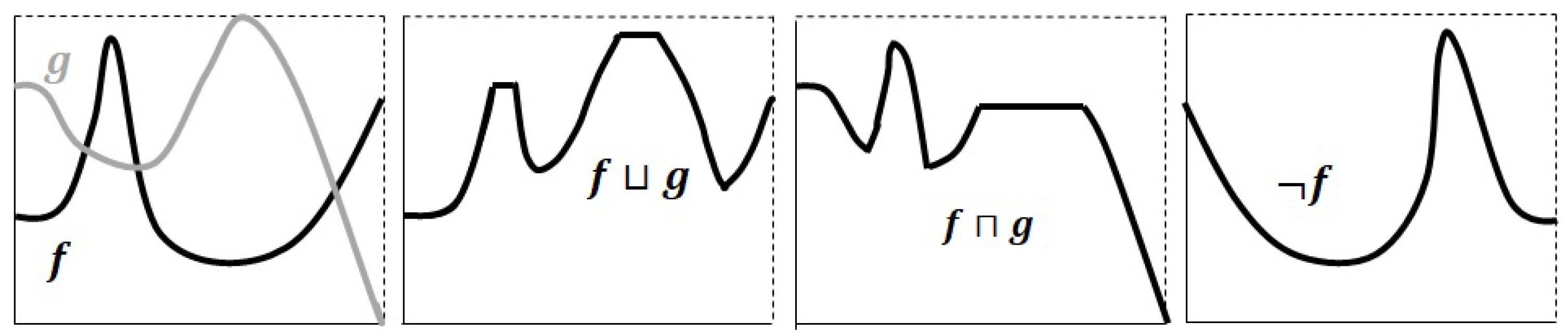
Figure 2.
([16], Fig. 7) Examples of and .
Figure 2.
([16], Fig. 7) Examples of and .
Disclaimer/Publisher’s Note: The statements, opinions and data contained in all publications are solely those of the individual author(s) and contributor(s) and not of MDPI and/or the editor(s). MDPI and/or the editor(s) disclaim responsibility for any injury to people or property resulting from any ideas, methods, instructions or products referred to in the content. |
© 2024 by the authors. Licensee MDPI, Basel, Switzerland. This article is an open access article distributed under the terms and conditions of the Creative Commons Attribution (CC BY) license (http://creativecommons.org/licenses/by/4.0/).
Copyright: This open access article is published under a Creative Commons CC BY 4.0 license, which permit the free download, distribution, and reuse, provided that the author and preprint are cited in any reuse.


