
Submitted:
12 November 2024
Posted:
13 November 2024
You are already at the latest version
Abstract
Addressing global warming and adapting to the impacts of climate change is a primary focus of Climate Change Adaptation strategies at both European and national levels. Land surface temperature (LST) is a widely used proxy for investigating the climate-change-induced phenomena, providing insights into the surface radiative properties of different land cover types and the impact of urbanization on local climate characteristics. Accurate and continuous estimation across large spatial regions is crucial for the implementation of LST as an essential parameter in climate change mitigation strategies. Here, we propose a deep-learning-based methodology for LST estimation using multi-source data, including Sentinel-2 imagery, land cover, and meteorological data. We develop a regression-based Convolutional Neural Network model, trained on ECOSTRESS mission data, which performs pixelwise LST predictions using 5×5 image patches, capturing contextual information around each pixel. This method not only preserves ECOSTRESS's native resolution but also fills data gaps, enhances spatial and temporal coverage, and provides LST predictions with at least 80% of all pixel errors that fall within a ±3°C range. Unlike traditional satellite-based techniques, our model leverages high-temporal-resolution meteorological data to capture diurnal variations, allowing for more robust LST predictions across different regions and time periods. The model's performance demonstrates the potential for integrating land surface temperature into urban planning, climate resilience strategies, and near-real-time heat stress monitoring, providing a valuable resource to assess and visualize the impact of urban development and land use and land cover changes.
Keywords:
climate change adaptation
; urban heat island
; land surface temperature
; ECOSTRESS
; Sentinel-2
; INCA
; convolutional neural network
1. Introduction
Responding to global warming and adapting to climate change effects such as heat waves and drought is a key priority of stakeholders involved in the definition of Climate Change Adaptation strategies [1]. Most of the largest cities experience profound changes due to urbanization and hence, city administrations are facing challenges in safeguarding high-quality urban growth despite increasingly tight spatial resources. Studies have shown that the degree of surface sealing has a direct impact on the radiation balance – by modifying the surface radiative properties and radiatively active air pollutants [2,3], thus influencing the ratio between sensible and latent heat fluxes. These modifications in the built-up environment make cities (but also smaller municipalities) warmer than their surroundings and more prone to excess heat, leading to an urban heat island effect [4]. Other studies have demonstrated that the temperature within urbanized areas shows a high degree of variability depending on the local urban morphology [5,6,7]. Land use and land cover, along with their changes in general, influence the local climate characteristics [8]. Regional and city administrations make use of this knowledge, aiming to reduce health risks related to climate change and to increase human well-being by implementing heat mitigation measures such as green and blue infrastructure [9]. Altering thermal comfort in urban environments enhances time of exposure to an uncomfortable amount of heat. This can be particularly dangerous for vulnerable individuals, as well as for those performing strenuous physical work in high heat, potentially leading to fatal outcomes [10,11]. Moreover, recent studies have highlighted that climate change in general, and increasing temperatures in particular, pose a significant risk for mountainous areas, affecting alpine communities and their economy (e.g., tourism) [12]. Global and regional warming can further amplify the effect of excess heat [13]. Taking adaptive measures is not only the focus of larger cities but also of any urban area and mountainous regions. Understanding how land use and climate trends impact local climates is essential for decision-makers to develop cost-effective, evidence-based, and consistent solutions for sustainable cities and for rural and mountainous communities.
Land Surface Temperature (LST) is a broadly used proxy to investigate the Surface Urban Heat Island (SUHI) effect [4]. The positive correlation between LST and the degree of surface sealing [14,15] represents the intensity of the SUHI which, identical to the urban heat island effect, is higher in urban environments compared to rural areas [14]. The degree of surface sealing is also related to the Bowen ratio (; ratio between sensible and latent heat fluxes) [16]. Surfaces with higher Bowen ratio () indicate lower soil moisture availability [17], leading to an increase in LST, enhanced heat exchange by convection, and an increase in near-surface air temperatures [18], thus intensifying urban heat [14,15]. Conversely, surfaces with lower Bowen ratio () indicate higher soil moisture availability [17], which decreases LST and favors the evapotranspiration-driven cooling effect, leading to a decrease in near-surface air temperatures [19]. LST is a crucial parameter in numerous fields, including surface energy and water balance, ecology, agriculture, environment, climatology, meteorology, and hydrology [20,21,22], contributing to an overall understanding of Earth’s surface dynamics and the impact of climate trends. Improving our understanding of LST and its interplay with surface sealing, land cover, and meteorological conditions is thus paramount, with a wide range of applications involving Surface Heat Island, urban climate studies [23,24,25], drought monitoring [26], surface soil moisture and evapotranspiration estimation [27,28], and numerical weather prediction, to name a few.
A major advantage of using land surface temperature to investigate SUHI effect is its availability from gridded data (e.g., Earth-observation (EO)-based retrieval), which enables the analysis of local effects depending on the resolution of the satellite sensor. In addition, remote-sensing-based LST dataset has been accepted by the International Geosphere and Biosphere Program as one of the high-priority parameters , and the Global Climate Observing System identified it as an Essential Climate Variable [30]. EO-based LST represents the accumulative radiometric surface temperature of all materials of the surface cover within the sensor’s field of view [31]. Thus, LST estimation from thermal infrared images is complex due to the surface composition, with materials of varying emissivity and geometry [32,33,34]. For example, a densely vegetated area represents the surface temperature of vegetation; whereas in a sparsely vegetated area, the surface temperature includes contributions from vegetation and soil simultaneously [33]. EO-based retrieval of land surface temperature has a long tradition dating back to the 1960s with the launch of the TIROS-II satellite [35,36]. Numerous EO sensors subsequently followed, carried on geostationary and low-Earth-orbit satellites and providing data at coarse spatial resolutions (750 m to 4 km, e.g., GOES, SEVIRI, AVHRR, MODIS, AATSR, VIIRS, Sentinel-3 SLSTR). Medium spatial resolution data (70 to 100 m) is offered through the sensors such as the Advanced Spaceborne Thermal Emission and Reflection Radiometer (ASTER), the Landsat Thermal Infrared Sensor (TIRS), and the ECOsystem Spaceborne Thermal Radiometer Experiment on Space Station (ECOSTRESS).
Satellite-based land surface temperature datasets have been extensively used, e.g., for advanced assessments of urban heat island effects – overcoming the challenges of conducting high-resolution air temperatures at similar scale [23], in assessment and mitigation studies elaborating on the spatiotemporal behavior of the urban heat islands [37,38,39,40,41,42,43], and in downscaling studies, providing high-resolution LST maps based on the assumption of a scale-invariant relationship between LST and other influencing parameters (e.g., surface sealing degree, reflectance, spectral indices) [42,44,45,46]. These advances establish land surface temperature as an essential parameter for advanced applications in urban and built-up environments. A particularly interesting approach consists of integrating methods operating at different scales to enhance modelling capabilities in heat assessment studies; namely, the integration of LST datasets with the Computational Fluid Dynamics (CFD)-GIS integrated modelling approach [6,7] – enabling modelling of the SUHI effect at very high spatial resolution, and urban climate models used to downscale and evaluate localized effects of heat or other climate-related parameters [47]. A critical requirement for fully utilizing LST within a multi-resolution and multi-sensor data fusion methodology is access to a comprehensive, high-quality LST dataset. Specifically, developing an inventory of LST data at high spatial and temporal resolution is a timely task. Such an inventory would be an important asset in multi-sensor methodologies at large scales (national, regional), enabling consistent analysis of various built-up environments, from small settlements to large cities.
Over the past decade, deep learning models have become integral to the field of Earth observation, providing cutting-edge tools for the exploration and handling of complex remote sensing datasets. Numerous pivotal reviews highlight the breakthroughs in remote sensing, demonstrating the advantages of deep learning over traditional approaches in applications such as image processing, data fusion, time series analysis, object detection, and land cover mapping [48,49,50,51,52,53]. Most of the developed deep learning methodologies focus on scene classification and image segmentation tasks such as land cover and land use classification, change detection, and urban mapping [54,55,56]. Convolutional Neural Networks (CNNs) have been extensively employed for these tasks due to their ability to learn relationships between neighboring pixels in an image, enabling the extraction and learning of complex spatial features [48,49]. Despite the focus on classification and segmentation tasks, regression-based CNN models utilizing satellite imagery are becoming increasingly prevalent, facilitating the estimation of continuous data in environmental, urban, and agricultural contexts [51]. The varied applications include ice concentration estimation [57], quantification of bacterial bloom in water systems [58], soil moisture prediction [59,60], modelling of water quality indicators [61], and surface and air temperature prediction [53,62,63,64].
In this paper, we develop a Convolutional Neural Network framework for the estimation of land surface temperature from land cover and land change information, cloud-free Sentinel-2 data, and hourly meteorological data. The output of the model are land surface temperature maps at the native resolution of ECOSTRESS, accessible at any arbitrary point in time and location given the availability of meteorological data. The lightweight, regression-based CNN methodology designed to effectively fill gaps in the ECOSTRESS LST observations is the main contribution of this work, providing high-quality land surface temperature data over large spatial regions and with high temporal resolution. This establishes an enhanced, high-quality land surface temperature dataset, crucial for integration and use in sophisticated urban climate modelling approaches or spatial planning activities [6,7,47].
Our paper is organized as follows. In Section 2, we describe the areas of interest and the datasets used in this work. In Section 3, we provide details on the CNN methodology. In Section 4, we present the model results and analyze land surface temperature predictions in spatial and temporal contexts. The discussion and conclusions are provided in Section 5 and Section 6, respectively.
2. Areas of Interest and Datasets
2.1. Areas of Interest
We selected two areas of interest for our study (AREA I and II), covering various land cover classes within the urban, rural, and alpine environment.
AREA I, located at approximately 47.27° N and 11.39° E and covering 19.3 × 16.3 km2, includes the city of Innsbruck, Austria, and its surrounding area (see Figure 1). The city region includes the typical heterogeneous urban environments (such as buildings and roads), vegetated areas (parks, lawns), and bodies of water (rivers, lakes). The area outside of the city borders includes rural and agricultural features, as well as the typical alpine features such as mountainous terrain, forests, and meadows. Innsbruck has a humid continental climate with highly variable summers, and the June-July daily mean temperature of 18.9 °C [65].
AREA II, located at approximately 48.21° N and 16.37° E and covering 29.8 × 22.4 km2, includes the city of Vienna, Austria, and its surrounding area (see Figure 1). The city region is characterized by the typical urban areas, residential, commercial and industrial areas, as well as vegetated and water areas. The greater region also includes extensive agricultural surfaces and forests. Vienna has a borderline oceanic and humid continental climate with warm summers, and the June-July daily mean temperature of 21.2 °C [65].
The primary application of interest within our study being heat monitoring, we focus on the analysis of land surface temperature trends during summer months. Therefore, we define our time window of interest as the summer months of June, July, and August. For the preparation of datasets described in the following subsections, we focus on the data available from the years 2022 and 2023. The data obtained within such constraints is thus a representation of typical summer conditions in AREA I and AREA II.
2.2. Land Surface Temperature
The primary objective of this study is the development of a neural-network-based model capable of capturing and predicting dense land surface temperature time-series over large spatial regions. Achieving this goal strongly relies on the careful selection of input datasets, a crucial step that underpins the modeling process. In the input data selection, we have been guided by the established theoretical models for land surface temperature, which provide the essential framework for relating the land surface temperature to the various physical parameters characterizing the surface and the surrounding environment.
Land surface temperature is a key environmental metric that measures the radiative skin temperature of the Earth's surface. Unlike air temperature, which is typically measured at weather stations and reflects the atmospheric conditions above ground, land surface temperature encompasses the thermal infrared radiation emitted by the land surface. Consequently, it is strongly dependent on the atmospheric dynamics, global radiation, and the reflective and absorptive surface characteristics [6,66,67,68], with the dependence on these various surface and atmospheric parameters captured by a physical model [66,67]:
Here, denote the surface (air) temperature, represents the net all-wave radiation flux, represents the substrate heat flux, is wind speed, and is the Bowen ratio [16]. The model in Eq. (1) captures the fundamental relationships governing land surface temperature in relation to ambient and surface parameters. However, it is of limited practical use, its utility being constrained by the demand for precise calculations of multiple heat fluxes, a task that is often challenging and spatially limited. Instead, we opt for a more robust approach leveraging a neural-network-based methodology, as described in more detail in Section 3, and we base our selection of input parameters on the physical model given by Eq. (1).
In particular, the parameters represent variables dependent on ambient meteorological conditions, while the Bowen ratio elucidates the relationship between sensible heat and latent heat, depending on factors such as surface type (e.g., vegetation, water, urban), weather conditions, and time of day [69]. With our choice of input parameters, we carefully address and encompass the elements from the physical model into our neural network model, ensuring a model that is both physically meaningful and computationally robust.
2.3. Input Datasets
The modelling workflow presented in this study makes use of multiple datasets, which are summarized in Table 1 and described in more detail in the following subsections. The thermal data consists of the ECOSTRESS 70 m LST product (Section 2.3.1). The meteorological data is provided by the Integrated Nowcasting through Comprehensive Analysis (INCA) dataset of the Austrian national meteorological service (Section 2.3.2), and the optical multispectral data includes Sentinel-2 imagery (Section 2.3.3). Additional land cover and topographic datasets are described in Section 2.3.4.
2.3.1. ECOSTRESS: Label Dataset
ECOSTRESS (ECOsystem Spaceborne Thermal Radiometer Experiment on Space Station) is an ongoing NASA scientific mission mounted on the International Space Station (ISS). The main instrument in ECOSTRESS is a multispectral thermal infrared radiometer, which collects and provides measurements of the surface temperature [70]. We use the ECOSTRESS Land Surface Temperature and Emissivity (ECOSTRESS-LSTE) Level 2 dataset for the supervised learning approach. The ECOSTRESS-LSTE L2 product is provided on 70 m resolution, with irregular revisit times of one to five days according to the flight pattern of the ISS [71]. Due to the inclined and precessing orbit of the ISS, observation times of the ECOSTRESS instrument vary, with some days providing multiple observations per day [72]. Spatially, the ECOSTRESS observations usually cover a large geographic area; specifically, a single ECOSTRESS-LSTE observation is typically sufficient to reproduce a single scene over our areas of interest. ECOSTRESS-LSTE is the cornerstone dataset of our model, providing labels for the supervised learning of the land surface temperature.
The corresponding ECOSTRESS data acquisition follows via an automated download directly from the NASA search portal [73]. The raw swath data is transformed into gridded single-band images in the Universal Transverse Mercator (UTM) projection using the open-source swath2grid conversion algorithm [74]. Particularly, we extract the land surface temperature (LST) and the quality control (QC) layers. The georeferenced LST layer is passed through several quality assessments and artifact mitigation steps. First, we make use of the intrinsic QC layer to mask out any low-quality pixels. The QC unsigned 16-bit data are stored as bit flags in the layer, with flags related to data quality, cloud, Temperature and Emissivity Separation (TES) algorithm diagnostics, and error estimates [70]. For the purposes of this study, we mask the LST layer by keeping only the best quality, cloud-free pixels, corresponding to the value for QC bits 1&0 = 00. This step is generally sufficient to eliminate most artifacts and clouds appearing in the observations. Second, we perform further manual checks to evaluate (i) the accuracy of georeferencing, and (ii) the quality of the QC masking. (i) In the case of georeferencing offset of more than 50 m, the image is labeled as incorrect and discarded from further analysis. (ii) In the case of insufficient cloud masking (identified by extremely low negative temperatures), custom additional masking is performed.
The LST dataset obtained after filtering suffers minimal issues due to incorrect georeferencing and undetected cloud coverage. As the result of the filtering, the data availability is reduced, leading to aperiodic availability of observations, and a typical 2–5-day revisit period in a specific location. The filtered ECOSTRESS LST data comprises the final dataset supplied to our model as the training reference labels. An example ECOSTRESS LST observation is shown in Figure 2 (a).
2.3.2. INCA
The INCA (Integrated Nowcasting through Comprehensive Analysis) dataset is a temporally detailed meteorological dataset provided by the Central Institute for Meteorology and Geodynamics (ZAMG) in Austria. The INCA data is modeled using various available data sources – station observations, remote sensing data, numerical weather prediction models and a high-resolution terrain model – to produce the analysis of the current state of the near-ground atmosphere [75]. INCA data is provided at a 1 km spatial and an hourly temporal resolution, with historical data available dating back to 2013. The dataset covers five weather-relevant parameters which we consider as the input: air temperature, global radiation, relative humidity, and wind speed in two directions. An example INCA air temperature observation is shown in Figure 2 (b). This comprehensive coverage offers a view of weather conditions at any given location, and it provides many of the essential physical parameters required by the physical model in Eq. (1). Spatially, the INCA dataset primarily covers Austria and its surrounding regions, focusing particularly on the areas with complex terrain, such as the Alpine region [75].
Within our data processing workflow, we select the time window of interest, as specified in Section 2, and acquire the full spatial INCA dataset on an hourly resolution via an automated download directly from the GeoSphere Austria Data Hub [76]. From the raw downloaded data, we extract the observations which are temporally closest to the ECOSTRESS LST observations downloaded and prepared as described in Section 2.3.1, such that each extracted INCA observation corresponds to a single ECOSTRESS LST observation. The extracted images are resampled to the native ECOSTRESS resolution (70 m). Although such resampling does not add new information, it helps to smooth the images and facilitates a more systematic comparison with the ECOSTRESS data.
The INCA data is provided on a much coarser resolution than ECOSTRESS (1 km compared to 70 m resolution). However, in the context of land surface temperature modelling this represents a sufficient input, as meteorological conditions are less spatially heterogeneous than the land surface characteristics. On the other hand, a nearly exact temporal matching is possible, due to the high hourly temporal resolution of the INCA dataset. As such, the INCA dataset meets our goal of relating the land surface temperature to the dynamic meteorological conditions at the time of the LST image acquisition.
2.3.3. Sentinel-2
The high-resolution input data for the land surface temperature mapping consists of the Sentinel-2 satellite data of the European Copernicus Earth observation program [77]. The Sentinel-2 mission provides high-resolution multispectral imagery, with spectral bands ranging from the visible to infrared part of the spectrum. Having a decametric resolution and a 5-day revisit time [77], the Sentinel-2 mission accurately captures the reflectance properties of surfaces around the time window of interest. It thus provides spatial information similar to, and more comprehensive than, the Bowen ratio parameter required in the physical model in Eq. (1). This makes it a crucial input for our model, enhancing its capability to analyze and interpret surface characteristics and providing a link between the land surface temperature and the various land cover classes.
For our data processing workflow, we select the Sentinel-2 images covering the area and time window of interest, and retrieve them locally from the Sentinel-2 Cloud Storage bucket [78]. We consider six spectral bands for the input (B2: Blue, B3: Green, B4: Red, B8: Near Infrared, B11 and B12: shortwave infrared), as well as the Scene Classification Layer (SCL) for the identification of clouds and shadow. An example Sentinel-2 B04 observation is shown in Figure 2 (c). Sentinel-2 imagery is divided into standardized 100 km × 100 km tiles. AREA I considered in our study is covered by the tile 32TPT, while AREA II is covered by the tiles 33UWP and 33UXP, with each tile having the projection of the 32 or 33 UTM zone (UTM/WGS84 projection). As the input for our model, we select and keep only the best available scenes, focusing on (i) mitigating cloud contamination and (ii) reducing data gaps due to swath overpass patterns, as the presence of any such low-quality areas in an image can negatively impact model training. To that end, we remove any of the images for which the metadata information indicates more than 10% cloud coverage. Additionally, we discard all the observations that contain more than 1% data gaps. Such filtering leads to, on average, 2-4 scenes available per tile and per summer.
Even though the filtering described above leads to a modest final number of total observations per tile, for the purposes of our analysis this is an adequate input. More specifically, these filtered images are a good representation of the average surface reflectance properties for the time window around which they were taken. As such, they are deemed sufficient to meet our goal of relating the land surface temperature to the more static surface properties, such as the land cover.
Finally, we match the selected Sentinel-2 observations to the ECOSTRESS LST and the matching INCA observations in several steps. (i) We resample (average) the Sentinel-2 images to the ECOSTRESS native resolution (70 m), (ii) we reproject ECOSTRESS and INCA images to the UTM projections, (iii) we clip ECOSTRESS and INCA images to each available Sentinel-2 tile, and (iv) we match any given ECOSTRESS/INCA tiled observation to the temporally closest Sentinel-2 observation.
2.3.4. Additional Input Datasets
In addition to the Sentinel-2 satellite imagery and the INCA meteorological data, in our approach we utilize several supplementary numerical datasets to enhance the robustness and the accuracy of the model. These include the European digital elevation model (EU-DEM) and derived parameters (slope, aspect), which provide detailed topographical characteristics [79], and several land cover datasets provided by the Copernicus Land Monitoring Service [80]:
- (i)
- tree cover density, a dataset which provides insights into vegetation distribution,
- (ii)
- water and wetness index, a dataset which indicates moisture levels and the presence of water bodies,
- (iii)
- imperviousness, a dataset which highlights the areas covered by artificial surfaces such as roads and buildings.
All the additional datasets are shown in Figure 2 (d–g). Combining these various additional layers with the optical and meteorological data accounts for environmental and land surface characteristics, thereby improving the overall modelling capability of our approach, and providing a link between land surface temperature and surface properties.
3. Methodology
3.1. Convolutional Neural Network Architecture for Pixelwise Regression
In this study we utilize a standard Convolutional Neural Network (CNN) model to perform pixelwise land surface temperature predictions based on the input features described in Section 2.3. Our model is adapted from the CNN configurations presented in [56,81], where a CNN architecture is developed for pixelwise segmentation and classification of Sentinel-2 imagery. Building upon this foundation, we have modified the architecture to address a continuous regression problem, enabling land surface temperature estimation.
The input to the pixelwise CNN consists of input features (described in Sections 2.3.2–2.3.4) spatially limited to a narrow image window (patch) around the pixel of interest. Adapting the approach in [56,81], we select a patch of size 5×5 as the input image to the CNN. At the native resolution of ECOSTRESS (70 m), this corresponds to a window of 350 m × 350 m, incorporating the contextual information surrounding each pixel. This inclusion of surrounding prominent features—such as vegetation, water bodies, agricultural fields, and industrial areas—enhances the model's ability to utilize and leverage contextual data during training.
The model architecture is shown schematically in Figure 3. We consider a network configuration consisting of a sequence of four 2D convolutional layers. Each layer performs a convolution with a 2×2 kernel and a stride of 1×1, using the rectifier activation function between layers. The stability and the performance of the model are enhanced by batch normalization layers incorporated after the second and the fourth convolutional layers [82]. Overfitting is mitigated by a subsequent dropout layer [83], which excludes 10% of the neurons during training. The final regression is done via a fully connected dense layer. The output layer has a size 1, utilizing linear activation to produce an output value that corresponds to the land surface temperature prediction for the central pixel in a patch. The network architecture and the relevant hyperparameters are summarized in Table 2.
The training dataset consists of nearly all summer observations, prepared as described in Section 2.3. One observation per year and per area of interest is excluded from the training dataset and used as the test dataset to evaluate the model’s performance after training. The ECOSTRESS data, detailed in Section 2.3.1, serves as the label data. For each area of interest, the training is carried out over the entire corresponding Sentinel-2 tile, namely, tile 32TPT for AREA I and tile 33UWP for AREA II.
3.2. Preparation of the Input Patches
Several steps are necessary to transform the input and label images into the image patches provided as the input to CNN. In the following we summarize the procedure for the training dataset, with the test dataset preparation being analogous. First, we generate 5×5 patches from all training and label images. For this, a sliding window of size 5×5 is applied, such that each pixel appears in a single patch only. Second, we filter the patches, keeping only those where all pixels in a patch have a valid value. This step eliminates patches with missing data in the ECOSTRESS images [as visible, e.g., in Figure 2 (a)], as well as patches with cloudy or shadowy pixels in the Sentinel-2 images, identified using the Scene Classification Layer (SCL). The input for the CNN is thus a multidimensional array of shape ×5×5×, and the labels are a multidimensional array of shape ×5×5. Here, denotes the total number of filtered patches across all summer observations considered for the training, and is the number of input features.
4. Results
4.1. Model Training
During the training phase, the input data is rescaled in the range [0,1] using the min-max scaling. The input data points are randomly shuffled into the training and validation datasets (used to evaluate the model’s performance during training), with the split ratio being 0.2. The configuration of the CNN and the hyperparameters used during training are outlined in Table 2. Training is performed for 50 epochs, with patches processed in batches of size 512. We utilize Adam stochastic optimization with inverse time decay, starting with an initial learning rate of 0.0001, which decays by a factor of 1 every 1000×(/512) steps. The model is optimized using the mean absolute error (MAE) as the loss function,
with and representing the predicted and the true LST value for each patch, respectively.
Once the model training is completed, the LST prediction is carried out over the unseen image in the test dataset. The test data is prepared in the same manner as described in Section 3.2, with the key difference being the use of a 1×1 sliding window to generate 5×5 patches for all non-border pixels in the image. This approach facilitates pixelwise predictions, allowing the creation of output images in a raster format that matches the resolution of the input images.
4.2. Performance Evaluation
We assess the model and its generalization capabilities by generating the LST predictions on the test dataset consisting of the images unseen by the model. More precisely, no pixel patches belonging to the test dataset were provided to the CNN for the training. These predictions are compared with the corresponding ECOSTRESS observations to evaluate the performance.
It is important to highlight a key distinction between the generation of the test and validation datasets. The validation dataset is a subset of filtered pixel patches derived from the train/validation split. In contrast, the test dataset is created by excluding an entire image before the train/validation split. The validation dataset is thus less distinct from the training dataset than the test dataset. As a result, predictive performance of the model on the test data provides a more accurate indication of the model’s generalization ability compared to the validation data. This is particularly relevant for assessing the model’s extrapolation capabilities, where "extrapolation" refers to making predictions on data points that fall outside the range of the training data, such as predicting LST in high-temperature scenarios with the model trained on lower-temperature observations.
For more comprehensive analysis, we assess the model over different training datasets by varying the hour range of the observations to be chosen for the training. Therefore, besides using training datasets with observations spanning the entire day, we also consider training datasets limited to smaller hour ranges at different times of the day, like for examples ranges falling in the morning or in the afternoon. Note that, due to the temporal scarcity of ECOSTRESS data, to prevent underfitting most of the available data (within the chosen hour range) must be used for training.
4.3. Qualitative Analysis of the Predictions
We begin by conducting a visual evaluation of the model predictions. In this qualitative assessment, the results are generally promising, as the model predictions closely resemble the ECOSTRESS measurements (see Figure 4 for examples of predictions over AREA I and AREA II). While some visual discrepancies do occur, they are typically limited to small, isolated patches of pixels, which constitute a minor portion of the overall image and are usually located outside of urban areas. These artifacts may originate from occasional model errors or input data issues (e.g., cloud interference). Despite this, the model predictions effectively capture the spatial features present in the ECOSTRESS observations, often further enhancing spatial detail by increasing contrast — particularly noticeable in features like rivers (cf. ECOSTRESS observations and the corresponding model predictions in Figure 4). The improvement in spatial detail is largely due to the integration of higher-resolution input data, which provides additional fine-scale information.
Additionally, the model exhibits strong ability to fill various gaps in the ECOSTRESS observations, including those caused by cloud cover, image border limitations, and grid-pattern sensor artifacts. These gaps, visible in Figure 4 (a,c), are effectively addressed by the model, as shown in Figure 4 (b,d). A close-up of typical ECOSTRESS grid artifacts is shown in Figure 5 (a), and the corresponding correction by the model, as well as the enhancement of spatial detail, is demonstrated in Figure 5 (b).
Overall, the visual analysis shows that the model not only replicates the spatial features of ECOSTRESS observations, but it also enhances detail and effectively fills various gaps appearing in the observations. These strengths highlight the model's potential for addressing common issues in remote sensing datasets and improving the accuracy of land surface temperature predictions.
4.4. Quantitative Analysis of the Predictions
For the statistical analysis, we consider all the pixelwise LST pairs, consisting of the prediction value and the corresponding ECOSTRESS measurement, within a single Sentinel-2 tile. To ensure valid comparisons, we include only the pairs where both pixels contain valid data. As a result, predictions for pixels lacking valid ECOSTRESS observation data are excluded from the analysis. Each prediction is evaluated based on the prediction error,
The following metrics are subsequently derived to obtain the statistics and the error distribution within a tile: (i) mean error (ME) and mean absolute error (MAE), (ii) coefficient of determination , (iii) minimum (min) and maximum (max), (iv) standard deviation (std), and (v) percentiles.
In our focus on urban applications, we prioritize MAE – a metric used as the loss function during training [see Eq. (2)] – as the key statistic for validating the predictions. While the maximum acceptable MAE varies depending on the specific application, a general guideline is that an MAE should not exceed 3°C, with no more than 25% of the pixelwise absolute error above this threshold. This standard aligns with recent studies investigating various machine learning approaches for estimating land surface temperature [63], as well as a milestone survey referenced therein [68].
Additionally, we compute the score, a scale-independent metric that indicates model fit, ranging from 1 (perfect fit) to 0 (mean fit), with negative values indicating poor fits. While is a valuable metric for evaluating performance, it can be challenging to interpret in isolation. In particular, an acceptable value depends on the explainable data variability and the signal-to-noise characteristics, as well as the intention to model the underlying pattern and avoid overfitting. While there is no universal standard for acceptable values in land surface temperature modeling, remote sensing studies typically consider values above 0.5–0.7 as acceptable, with a preference for higher values up to 0.9–0.95, above which the chance of overfitting increases. Note that there is no direct relationship between MAE and ; low MAE can coexist with low and vice versa. Finally, to ensure a comprehensive analysis, we include minimum, maximum, and percentile values to provide a more complete picture of model performance.
A total of 22 image predictions on test data are computed and evaluated. Table 3 summarizes the statistics for the predictions with the 4 best and 4 worst resulting MAE. Note that the predictions are not all derived from the exact same trained model. Instead, they are derived from different realizations of the model yielded by training on observations spanning different hour ranges (as discussed in Section 4.2). The bottom row in each tile cell displays ensemble statistics, computed for all pixels across all 22 predictions. The ensemble statistics provide a comprehensive assessment of the model's overall predictive performance, as opposed to evaluating individual predictions based on specific datasets or single training instances. It is important to highlight that the ensemble MAE represents the weighted average of the single prediction MAEs based on pixel count. However, this statement does not apply to all statistics, and percentiles.
As shown in Table 3, the ensemble MAE for tile 32TPT is 1.93°C, with the 10th and 90th percentiles at -2.59°C and +3.16°C, respectively. The ensemble MAE for tile 33UWP is 1.60°C, with the 10th and 90th percentiles at -2.68°C and +2.27°C, respectively. This means that at least 80% of the pixel errors fall within the ±3°C range, with only a slight deviation for the 90th percentile in 32TPT. The slightly worse performance over the 32TPT tile could reflect the more complex microclimate and surface conditions of the alpine environment in AREA I, which increases variability in the temperature data and leads to a broader error distribution. In contrast, the flatter urbanized conditions in AREA II lead to more stable LST patterns, resulting in a narrower error range. Despite this, the error margins in both locations fall well within acceptable limits. Additionally, the ensemble values of 0.87 for both tiles indicate a robust overall fit and a strong correlation between the model predictions and the ECOSTRESS data, despite some individual predictions having lower . Finally, it is important to note that maximum overestimation and underestimation errors at individual pixels can occasionally reach extreme values, with some predicted temperatures falling outside reasonable ranges (refer to the max and min columns in Table 3). Such errors are primarily outliers; they correspond to the artifacts reported in the qualitative analysis in Section 4.3 and have a limited impact on overall predictive performance. They could be mitigated through targeted postprocessing techniques, ensemble learning (i.e., combining predictions from multiple models), or by flagging these data points as invalid.
Figure 6 provides further analysis of the LST distributions for the two prediction ensembles, displayed through histograms and bivariate histograms. Panels (a) and (c) compare the predicted with observed LST distributions for tiles 32TPT and 33UWP, respectively. While the two datasets do not align perfectly, the model generally captures the mayor temperature peaks in terms of both width and height, indicating reasonable agreement. The bivariate histograms in panels (b) and (d) further reveal the relationship between the predicted and the true LST values in 33TPT and 33UWP, respectively. Most data points fall along the diagonal, confirming strong overall agreement, though some outliers are present. These deviations may originate from systemic data issues such as unmasked clouds (thin linear artifacts in the histograms), or from a model tendency to overestimate low LST values in alpine areas [a larger concentration of outliers present in panel (b)].
We considered models trained on different time windows to derive the 22 predictions evaluated in Table 3. In particular, we considered full-day and afternoon models trained on observations spanning, respectively, the entire day and afternoon hours. To assess the impact of the training data time window on the model performance, in Table 4 we compare the ensemble statistics for the predictions which are derived from the full-day model with those derived from afternoon models. While the MAE is slightly lower for the afternoon models, values are similar. This indicates that the full-day model is less accurate than the afternoon models, while they explain data variability equally well. However, the error distribution for the full-day model is significantly more spread, with higher maximum overestimation and underestimation errors. In fact, the full-day model mostly contributes to the lower performance metrics in Table 3. Despite having more data for training, the full-day model thus performs worse overall than the narrower afternoon model. This is likely a sign that the relationship between the considered input features (e.g., air temperature, etc...) and LST changes with the time of the day. The input features include in fact only atmospheric conditions at a single point in time, whereas time-series are likely to determine the LST.
For completeness, in Figure 7 we display the LST distributions for the afternoon model prediction ensembles for tiles 32TPT and 33UWP, which can be directly compared with Figure 6. The histograms in panels (a) and (c) show a similarly reasonable agreement as seen in Figure 6, with the morning-related lower temperature peaks now absent. The bivariate histograms in panels (b) and (d) demonstrate improved correlation and fewer outliers, indicating a stronger alignment between predictions and observations compared to the full-day model prediction ensembles.
Finally, all predictions discussed so far are generated within the same time range as the training data. We also evaluate the model's performance when extrapolating beyond this range, such as generating morning predictions from afternoon models, with the results summarized in Table 5. The accuracy for these extrapolated predictions is significantly lower compared to interpolated ones. This is somewhat expected, given the inherent challenges of extrapolation. Nonetheless, the statistics remain close to the acceptable bounds, with approximately 80% of the pixel errors falling within the ±5°C range. This suggests a robust and consistent relationship between input features and LST, with minimal variations between morning and afternoon predictions. However, for more fine-scale modeling and improved accuracy, such extrapolation is not sufficient.
5. Discussion
5.1. Application of the Data Fusion Approach
In our proposed approach, we employ a CNN model for pixelwise land surface temperature predictions at moderate to high spatial resolution (i.e., 70 m) combining multi- source and multi-resolution input features (i.e., coarse resolution reanalysis data from a meteorological nowcasting prediction system, high-resolution land cover data, high-resolution multi-spectral optical satellite data) to gap-fill and densify remote-sensing-based LST observations. The CNN model is trained based on the ECOSTRESS-LSTE L2 dataset provided via the NASA Earthdata portal. The model makes use of the 5×5 input pixel patches, corresponding to a 350 m × 350 m area at the native resolution of ECOSTRESS, incorporating surrounding contextual information such as vegetation cover and water bodies to enhance prediction accuracy. The advantage of the proposed methodology compared to conventional and purely remote sensing-based techniques is that the model-based approach combines the superior dense temporal sampling of the meteorological model data with the substantially higher spatial detail of the remote-sensing-based LST observations. Having such a model in place allows us to get dense LST estimates at a high spatial resolution to support a variety of applications like supporting local spatial planning authorities in identifying hotspot regions within urban environments, analyzing the context between land use and land cover and associated heat impact, or supporting the development of local, near-real-time heat stress warning systems by exchanging the reanalysis data with numerical weather prediction parameters, to name a few. Having such applications in mind, the prediction accuracy (i.e., observed and MAE) of our model is good and allows to highlight and analyze spatial variability and temperature contrasts between various land cover types.
The advantage of our method compared to other approaches which purely rely on remote-sensing-based LST estimates and data cross-calibration (e.g., [44]) is two-fold. First, due to the strong diurnal variations of LST mainly depending on the meteorological conditions, fusing data from various satellite sensors to gap-fill LST data requires sophisticated inter-calibration techniques to correct for LST differences caused by different overpass times. Thus, using meteorological reanalysis data from a highly resolved numerical weather prediction (NWP) model with similar spatial resolution like coarse resolution satellite-based LST estimates (e.g., Sentinel-3, MODIS, VIIRS) has the advantage of offering the meteorological conditions for any observation time and already incorporating a physical-based treatment of meteorological processes. Second, due to the superior temporal sampling of the NWP model outputs, our trained model can be applied to any time step and is less dependent on satellite flight schedules and revisit times, finally enabling us to create a more representative LST dataset which provides comparability between regions over large scales. Furthermore, the NWP output can also be replaced with the output from Regional Climate Models (RCMs) to analyze and evaluate future climate change impacts. Alternative approaches (e.g., [84]) make use of geostationary satellite imagery (e.g., MSG SEVIRI, GOES) to gap-fill LST data, which offers hourly or even sub-hourly temporal observations. Yet, they typically have a larger Ground Sample Distance (~ 5 km in mid-latitudes) then the above-mentioned polar-orbiting instruments (~ 1 km) and cannot be considered for the RCM approach in the context of climate change adaptation studies.
Other studies have successfully used multi-source data fusion to gap-fill LST by incorporating land surface models [85] and applying deep learning techniques to fuse remote sensing data with in-situ observations [64]. These approaches have demonstrated high spatial and temporal coverage with strong accuracy over specific areas and time windows of interest. Our approach complements these efforts by introducing a lightweight CNN model that is robust across time domains, allowing us to generate LST predictions consistently over a 3-month summer period. This flexibility enables the creation of long-term, high-density LST datasets for any region with available meteorological data, facilitating the development of near-real-time LST monitoring systems that can be seamlessly implemented for real-time applications.
5.2. Limitations of the Deep Learning Model
While the model demonstrates generally good performance, there are several limitations that affect its accuracy and reliability. One of the main issues observed is the occurrence of over- and underestimation errors at individual pixels, as reflected in the minimum and maximum values in the ensemble statistics (see Table 3). Although these errors are infrequent, they contribute to outliers that can affect the model's overall predictive performance. Tracing the exact source of these errors is challenging due to the intricate relationships between input features – such as land cover, meteorological data, and satellite imagery – and land surface temperature, as well as the intrinsic complexities of deep-learning-based models. These errors could originate from the inherent variability in surface conditions (leading to a complex land surface temperature modelling response), from the inconsistencies in the input data (e.g., unmasked clouds, noise, and other artifacts), or from model architecture limitations. While the calculated ensemble MAEs for both tiles remain within acceptable limits, addressing these outliers could further enhance accuracy. Potential approaches that could help improve error management and provide a more robust and interpretable framework include tailored postprocessing techniques, ensemble learning, or hybrid models which incorporate additional physical constraints.
The performance of the model is also impacted when trained on the data spanning an entire day, as demonstrated by the comparison of the full-day and the afternoon ensemble statistics (see Table 4). Specifically, the full-day model tends to exhibit poorer performance compared to models trained on specific time ranges, such as afternoon-only datasets, despite having generally more data available for training. This difference is likely due to the dependency of the LST on the input features changing with the time of the day, as more complex time-series dynamics in such relationship are not considered in our model. Consequently, the full-day model exhibits a more spread error distribution, with higher maximum over- and underestimation errors.
Another limitation stems from the scarcity and uneven quality of ECOSTRESS data available for training. The limited availability of good-quality observations affects the model's ability to generalize, particularly in cases where predictions are made outside the training data time range. For instance, morning predictions from models trained on afternoon data show worse statistics than interpolated predictions, but they remain within acceptable limits. Extrapolation, in general, proves to be more error-prone than interpolation due to the model's inability to fully capture diurnal variations in LST.
5.3. ECOSTRESS Data Quality
We encountered several data quality issues when collecting the ECOSTRESS-LSTE data for both areas of interest. These issues are primarily observed in the form of missing data due to cloud contamination, and artifacts and georeferencing inconsistencies, which can impact the reliability of the data. Applying the associated ECOSTRESS quality mask (provided by the QC layer in the ECOTRESS-LSTE dataset) helps mitigate some of these issues.
The quality issues affecting the ECOSTRESS dataset can be divided into three categories: (i) instrument artefacts, (ii) incorrect georeferencing, and (iii) QC layer insufficiencies. (i) Instrument artifacts are a prominent issue, appearing as stripes (linear or grid-like patterns disrupting data uniformity) and grooves (irregular indentations affecting data consistency), as illustrated in Figure 8 (a). These artefacts are caused by damage to the TIR sensor during pre-launch testing [86]. They are an intrinsic property of the ECOSTRESS dataset, arising from the issues in the sensor itself, and as such, they cannot be eliminated. However, as shown in the visual analysis in Section 4.3, the CNN model is able to correctly identify and mitigate these artifacts effectively (see, e.g., Figure 5). (ii) Another significant issue is inconsistent or incorrect georeferencing, as provided by the ECOSTRESS-GEO geolocation dataset within the swath2grid algorithm (see Section 2.3.1 for details). As illustrated in Figure 8 (a), incorrect georeferencing appears as misalignment between LST data and geographic coordinates, while inconsistent georeferencing refers to variability in spatial accuracy across different observations. This issue is sporadic and unpredictable, and developing an automated correction procedure is beyond the scope of this work. In our processing workflow, we addressed this by reviewing all observations in the training dataset and excluding those with inaccurate georeferencing from further analysis, as the accuracy of the deep learning model depends on the quality of the label data (i.e., ECOSTRESS LST). (iii) The original ECOSTRESS QC mask is intended to filter out unreliable data. However, it is not always sufficient and can introduce further complications such incorrect cloud masking, leading to erroneous temperature readings. Specifically, the QC mask occasionally failed to fully remove cloud cover, leading to unrealistic temperature gradients and misleading thermal readings due to partial cloud obstruction. An example of this issue is illustrated in Figure 8 (b-c), where a cloud is not correctly masked. To address this, we screened the QC data and added additional manual masking in observations with significant cloud masking artifacts.
Despite our efforts to mitigate ECOSTRESS data quality issues, some of the observed prediction artifacts (such as the significant under- or overestimation errors reported in Table 3) may still originate from undetected low-quality data used for the model training. Similar data filtering and quality issues with ECOSTRESS datasets have been reported in previous studies [86,87].
5.4. Future Directions
Planned future directions include efforts to enhance the spatial resolution of LST predictions, specifically by exploring techniques to downscale LST to 10-meter resolution. This approach will explore the scaling effects characteristic to downscaling, reported in previous studies [44,45,46], as well as deep learning based methodologies to overcome these issues. Downscaled LST product provided at high temporal resolution and spatial coverage would provide more detailed insights, particularly in urban environments where fine-scale temperature variations are critical for local climate analysis and planning.
Furthermore, the inclusion of in-situ temperature measurements to validate and complement remote sensing LST data should be considered. Planned ground truth validation activities focus on using data from the black ice monitoring system in Upper Austria, where sensors embedded in roads provide high-precision point measurements of surface temperature. Despite these data being limited to one surface type, they serve as valuable reference points for model validation. By integrating in-situ data, future studies can bridge the gap between modeled predictions and real-world conditions, thus providing more robust datasets for urban heat monitoring. Additionally, model comparisons are planned using satellite-derived datasets from commercial satellite operators like OroraTech [88] and Constellr [89], although alignment between timestamps and resolutions remains a challenge.
Finally, a thorough evaluation of the INCA (Integrated Nowcasting through Comprehensive Analysis) dataset should be conducted, as it is a model-based system. Since it is a crucial dataset in attaining the temporal gap-filling and density of the LST predictions, its performance as a predictor for LST estimation is crucial and could affect overall model accuracy. Ensuring the reliability of input models like INCA is crucial for improving the predictive quality of downstream applications.
6. Conclusions
This study presents a deep learning-based methodology for estimating land surface temperature (LST) using a combination of multi-source and multi-resolution meteorological, land cover, and satellite data, including the ECOSTRESS LST data. The proposed Convolutional Neural Network model demonstrates promising results in generating a gap-filled LST time series over large areas at medium to high spatial resolution (<100 m). We showed that the generated LST predictions lead to at least 80% of the pixel errors falling within an acceptable ±3°C range. Unlike traditional satellite-based techniques, our model leverages high-resolution meteorological data to capture diurnal variations, allowing for more robust LST predictions across different regions and time periods. The proposed methodology is timely and can be applied to a variety of fields including urban planning, climate resilience, and real-time heat stress monitoring, with the goal of supporting spatial planning and climate change adaptation activities.
While the model offers robust performance over extended time periods and large areas, several challenges remain, particularly in terms of error traceability, ECOSTRESS data quality, and limitations related to model-based inputs such as INCA. Future work should focus on addressing these limitations by integrating ground truth measurements for improved validation. Through continued refinement and validation, the approach holds significant potential to support climate adaptation strategies and to improve our understanding of land use and climate interactions.
Author Contributions
Conceptualization, M.R. and K.K.; methodology, K.K. and D.C.; software, K.K. and D.C.; validation, D.C.; formal analysis, K.K. and D.C.; investigation K.K. and D.C.; resources, K.K. and D.C.; data curation, K.K.; writing—original draft preparation, K.K., D.C. and M.R..; writing—review and editing, M.R., K.K. and M.S..; visualization, K.K. and D.C.; supervision, M.R. and M.S..; project administration, M.S.; funding acquisition, M.R. All authors have read and agreed to the published version of the manuscript.
Funding
We would like to thank the European Space Agency (ESA) for funding the project “HeatAdapt: Monitoring and mitigating heat hotspot areas”, under which the presented research has been conducted.
Data Availability Statement
The data that support the findings of this study are openly available at https://gtif.esa.int.
Acknowledgments
The authors are grateful for the fruitful and illuminating discussions with Patrick Griffiths and Francesca Elisa Leonelli.
Conflicts of Interest
The authors declare no conflicts of interest.
References
- Turek-Hankins, L.L.; Coughlan de Perez, E.; Scarpa, G.; Ruiz-Diaz, R.; Schwerdtle, P.N.; Joe, E.T.; Galappaththi, E.K.; French, E.M.; Austin, S.E.; Singh, C.; et al. Climate Change Adaptation to Extreme Heat: A Global Systematic Review of Implemented Action. Oxford Open Climate Change 2021, 1, kgab005. [Google Scholar] [CrossRef]
- Oke, T.R. The Energetic Basis of the Urban Heat Island. Q. J. R. Meteorol. Soc. 1982, 108, 1–24. [Google Scholar] [CrossRef]
- Oke, T.R.; Mills, G.; Christen, A.; Voogt, J.A. Urban Climates; Cambridge University Press, 2017; ISBN 978-1-139-01647-6.
- Deilami, K.; Kamruzzaman, Md.; Liu, Y. Urban Heat Island Effect: A Systematic Review of Spatio-Temporal Factors, Data, Methods, and Mitigation Measures. Int. J. Appl. Earth Obs. Geoinf. 2018, 67, 30–42. [Google Scholar] [CrossRef]
- Logan, T.M.; Zaitchik, B.; Guikema, S.; Nisbet, A. Night and Day: The Influence and Relative Importance of Urban Characteristics on Remotely Sensed Land Surface Temperature. Remote Sens. Environ. 2020, 247, 111861. [Google Scholar] [CrossRef]
- Back, Y.; Bach, P.M.; Jasper-Tönnies, A.; Rauch, W.; Kleidorfer, M. A Rapid Fine-Scale Approach to Modelling Urban Bioclimatic Conditions. Sci. Total Environ. 2021, 756, 143732. [Google Scholar] [CrossRef]
- Back, Y.; Kumar, P.; Bach, P.M.; Rauch, W.; Kleidorfer, M. Integrating CFD-GIS Modelling to Refine Urban Heat and Thermal Comfort Assessment. Sci. Total Environ. 2023, 858, 159729. [Google Scholar] [CrossRef]
- Hart, M.A.; Sailor, D.J. Quantifying the Influence of Land-Use and Surface Characteristics on Spatial Variability in the Urban Heat Island. Theor. Appl. Climatol. 2009, 95, 397–406. [Google Scholar] [CrossRef]
- Kumar, P.; Debele, S.E.; Khalili, S.; Halios, C.H.; Sahani, J.; Aghamohammadi, N.; Andrade, M. de F.; Athanassiadou, M.; Bhui, K.; Calvillo, N.; et al. Urban Heat Mitigation by Green and Blue Infrastructure: Drivers, Effectiveness, and Future Needs. The Innovation 2024, 5. [Google Scholar] [CrossRef]
- Greene, S.; Kalkstein, L.S.; Mills, D.M.; Samenow, J. An Examination of Climate Change on Extreme Heat Events and Climate–Mortality Relationships in Large U.S. Cities. Wea. Climate Soc. 2011, 3, 281–292. [Google Scholar] [CrossRef]
- Vicedo-Cabrera, A.M.; Scovronick, N.; Sera, F.; Royé, D.; Schneider, R.; Tobias, A.; Astrom, C.; Guo, Y.; Honda, Y.; Hondula, D.M.; et al. The Burden of Heat-Related Mortality Attributable to Recent Human-Induced Climate Change. Nat. Clim. Chang. 2021, 11, 492–500. [Google Scholar] [CrossRef]
- Terzi, S.; Torresan, S.; Schneiderbauer, S.; Critto, A.; Zebisch, M.; Marcomini, A. Multi-Risk Assessment in Mountain Regions: A Review of Modelling Approaches for Climate Change Adaptation. J. Environ. Manag. 2019, 232, 759–771. [Google Scholar] [CrossRef] [PubMed]
- Intergovernmental Panel on Climate Change (IPCC) Climate Change 2022 – Impacts, Adaptation and Vulnerability: Working Group II Contribution to the Sixth Assessment Report of the Intergovernmental Panel on Climate Change; Cambridge University Press, 2023; ISBN 978-1-00-932584-4.
- Li, H.; Zhou, Y.; Li, X.; Meng, L.; Wang, X.; Wu, S.; Sodoudi, S. A New Method to Quantify Surface Urban Heat Island Intensity. Sci. Total Environ. 2018, 624, 262–272. [Google Scholar] [CrossRef] [PubMed]
- Yang, Q.; Huang, X.; Yang, J.; Liu, Y. The Relationship between Land Surface Temperature and Artificial Impervious Surface Fraction in 682 Global Cities: Spatiotemporal Variations and Drivers. Environ. Res. Lett. 2021, 16, 024032. [Google Scholar] [CrossRef]
- Bowen, I.S. The Ratio of Heat Losses by Conduction and by Evaporation from Any Water Surface. Phys. Rev. 1926, 27, 779–787. [Google Scholar] [CrossRef]
- Mahmood, R.; Pielke Sr., R. A.; Hubbard, K.G.; Niyogi, D.; Dirmeyer, P.A.; McAlpine, C.; Carleton, A.M.; Hale, R.; Gameda, S.; Beltrán-Przekurat, A.; et al. Land Cover Changes and Their Biogeophysical Effects on Climate. Int. J. Climatol. 2014, 34, 929–953. [Google Scholar] [CrossRef]
- Schwingshackl, C.; Hirschi, M.; Seneviratne, S.I. Quantifying Spatiotemporal Variations of Soil Moisture Control on Surface Energy Balance and Near-Surface Air Temperature. J. Climate 2017, 30, 7105–7124. [Google Scholar] [CrossRef]
- Li, D.; Liao, W.; Rigden, A.J.; Liu, X.; Wang, D.; Malyshev, S.; Shevliakova, E. Urban Heat Island: Aerodynamics or Imperviousness? Sci. Adv. 2019, 5, eaau4299. [Google Scholar] [CrossRef]
- Anderson, M.C.; Norman, J.M.; Kustas, W.P.; Houborg, R.; Starks, P.J.; Agam, N. A Thermal-Based Remote Sensing Technique for Routine Mapping of Land-Surface Carbon, Water and Energy Fluxes from Field to Regional Scales. Remote Sens. Environ. 2008, 112, 4227–4241. [Google Scholar] [CrossRef]
- Dash, P.; Göttsche, F.-M.; Olesen, F.-S.; Fischer, H. Land Surface Temperature and Emissivity Estimation from Passive Sensor Data: Theory and Practice-Current Trends. Int. J. Remote Sens. 2002, 23, 2563–2594. [Google Scholar] [CrossRef]
- Dickinson, R.E. Land Surface Processes and Climate—Surface Albedos and Energy Balance. In Theory of Climate; Elsevier: Berlin/Heidelberg, Germany, 1983. [Google Scholar]
- Zhou, D.; Xiao, J.; Bonafoni, S.; Berger, C.; Deilami, K.; Zhou, Y.; Frolking, S.; Yao, R.; Qiao, Z.; Sobrino, J.A. Satellite Remote Sensing of Surface Urban Heat Islands: Progress, Challenges, and Perspectives. Remote Sens. 2019, 11, 48. [Google Scholar] [CrossRef]
- Wesley, E.J.; Brunsell, N.A. Greenspace Pattern and the Surface Urban Heat Island: A Biophysically-Based Approach to Investigating the Effects of Urban Landscape Configuration. Remote Sens. 2019, 11, 2322. [Google Scholar] [CrossRef]
- Granero-Belinchon, C.; Michel, A.; Lagouarde, J.-P.; Sobrino, J.A.; Briottet, X. Night Thermal Unmixing for the Study of Microscale Surface Urban Heat Islands with TRISHNA-Like Data. Remote Sens. 2019, 11, 1449. [Google Scholar] [CrossRef]
- Cammalleri, C.; Vogt, J. On the Role of Land Surface Temperature as Proxy of Soil Moisture Status for Drought Monitoring in Europe. Remote Sens. 2015, 7, 16849–16864. [Google Scholar] [CrossRef]
- Sun, J.; Salvucci, G.D.; Entekhabi, D. Estimates of Evapotranspiration from MODIS and AMSR-E Land Surface Temperature and Moisture over the Southern Great Plains. Remote Sens. Environ. 2012, 127, 44–59. [Google Scholar] [CrossRef]
- Galleguillos, M.; Jacob, F.; Prévot, L.; French, A.; Lagacherie, P. Comparison of Two Temperature Differencing Methods to Estimate Daily Evapotranspiration over a Mediterranean Vineyard Watershed from ASTER Data. Remote Sens. Environ. 2011, 115, 1326–1340. [Google Scholar] [CrossRef]
- Townshend, J.R.G.; Justice, C.O.; Skole, D.; Malingreau, J.-P.; Cihlar, J.; Teillet, P.; Sadowski, F.; Ruttenberg, S. The 1 Km Resolution Global Data Set: Needs of the International Geosphere Biosphere Programme. Int. J. Remote Sens. 1994, 15, 3417–3441. [Google Scholar] [CrossRef]
- Belward, A.; Bourassa, M.A.; Dowell, M.; Briggs, S. The Global Observing System for Climate: Implementation Needs 2016.
- Yu, Y.; Liu, Y.; Yu, P. Land Surface Temperature Product Development for JPSS and GOES-R Missions. In Comprehensive Remote Sensing; Elsevier: Berlin/Heidelberg, Germany, 2018. [Google Scholar]
- Becker, F.; Li, Z. Surface Temperature and Emissivity at Various Scales: Definition, Measurement and Related Problems. Remote Sensing Reviews 1995, 12, 225–253. [Google Scholar] [CrossRef]
- Dash, P.; Göttsche, F.-M.; Olesen, F.-S.; Fischer, H. Retrieval of Land Surface Temperature and Emissivity from Satellite Data: Physics, Theoretical Limitations and Current Methods. J. Indian Soc. Remote Sens. 2001, 29, 23–30. [Google Scholar] [CrossRef]
- Qin, Z.; Karnieli, A. Progress in the Remote Sensing of Land Surface Temperature and Ground Emissivity Using NOAA-AVHRR Data. Int. J. Remote Sens. 1999, 20, 2367–2393. [Google Scholar] [CrossRef]
- Prata, A.J.; Caselles, V.; Coll, C.; Sobrino, J.A.; Ottlé, C. Thermal Remote Sensing of Land Surface Temperature from Satellites: Current Status and Future Prospects. Remote Sensing Reviews 1995, 12, 175–224. [Google Scholar] [CrossRef]
- Wark, D.Q.; Yamamoto, G.; Lienesch, J.H. Methods of Estimating Infrared Flux and Surface Temperature from Meteorological Satellites. J. Atmos. Sci. 1962, 19, 369–384. [Google Scholar] [CrossRef]
- Manoli, G.; Fatichi, S.; Bou-Zeid, E.; Katul, G.G. Seasonal Hysteresis of Surface Urban Heat Islands. Proc. Natl. Acad. Sci. U.S.A. 2020, 117, 7082–7089. [Google Scholar] [CrossRef] [PubMed]
- Dian, C.; Pongracz, R.; Dezső, Z.; Bartholy, J. Annual and Monthly Analysis of Surface Urban Heat Island Intensity with Respect to the Local Climate Zones in Budapest. Urban Clim. 2020, 31, 100573. [Google Scholar] [CrossRef]
- Benz, S.A.; Burney, J.A. Widespread Race and Class Disparities in Surface Urban Heat Extremes Across the United States. Earth’s Future 2021, 9, e2021EF002016. [Google Scholar] [CrossRef]
- Peng, S.; Piao, S.; Ciais, P.; Friedlingstein, P.; Ottle, C.; Bréon, F.-M.; Nan, H.; Zhou, L.; Myneni, R.B. Surface Urban Heat Island Across 419 Global Big Cities. Environ. Sci. Technol. 2012, 46, 696–703. [Google Scholar] [CrossRef]
- Sobrino, J.A.; Oltra-Carrió, R.; Sòria, G.; Jiménez-Muñoz, J.C.; Franch, B.; Hidalgo, V.; Mattar, C.; Julien, Y.; Cuenca, J.; Romaguera, M.; et al. Evaluation of the Surface Urban Heat Island Effect in the City of Madrid by Thermal Remote Sensing. Int. J. Remote Sens. 2013, 34, 3177–3192. [Google Scholar] [CrossRef]
- Zhou, J.; Liu, S.; Li, M.; Zhan, W.; Xu, Z.; Xu, T. Quantification of the Scale Effect in Downscaling Remotely Sensed Land Surface Temperature. Remote Sens. 2016, 8, 975. [Google Scholar] [CrossRef]
- Zhou, B.; Rybski, D.; Kropp, J.P. The Role of City Size and Urban Form in the Surface Urban Heat Island. Sci. Rep. 2017, 7, 4791. [Google Scholar] [CrossRef]
- Onačillová, K.; Gallay, M.; Paluba, D.; Péliová, A.; Tokarčík, O.; Laubertová, D. Combining Landsat 8 and Sentinel-2 Data in Google Earth Engine to Derive Higher Resolution Land Surface Temperature Maps in Urban Environment. Remote Sens. 2022, 14, 4076. [Google Scholar] [CrossRef]
- Pu, R. Assessing Scaling Effect in Downscaling Land Surface Temperature in a Heterogenous Urban Environment. Int. J. Appl. Earth Obs. Geoinf. 2021, 96, 102256. [Google Scholar] [CrossRef]
- Pu, R.; Bonafoni, S. Reducing Scaling Effect on Downscaled Land Surface Temperature Maps in Heterogenous Urban Environments. Remote Sens. 2021, 13, 5044. [Google Scholar] [CrossRef]
- Masson, V.; Heldens, W.; Bocher, E.; Bonhomme, M.; Bucher, B.; Burmeister, C.; de Munck, C.; Esch, T.; Hidalgo, J.; Kanani-Sühring, F.; et al. City-Descriptive Input Data for Urban Climate Models: Model Requirements, Data Sources and Challenges. Urban Clim. 2020, 31, 100536. [Google Scholar] [CrossRef]
- Zhu, X.X.; Tuia, D.; Mou, L.; Xia, G.-S.; Zhang, L.; Xu, F.; Fraundorfer, F. Deep Learning in Remote Sensing: A Comprehensive Review and List of Resources. IEEE Geosci. Remote Sens. 2017, 5, 8–36. [Google Scholar] [CrossRef]
- Ball, J.E.; Anderson, D.T.; Sr, C.S.C. Comprehensive Survey of Deep Learning in Remote Sensing: Theories, Tools, and Challenges for the Community. J. Appl. Remote Sens. 2017, 11, 042609. [Google Scholar] [CrossRef]
- Chlingaryan, A.; Sukkarieh, S.; Whelan, B. Machine Learning Approaches for Crop Yield Prediction and Nitrogen Status Estimation in Precision Agriculture: A Review. Comput. Electron. Agric. 2018, 151, 61–69. [Google Scholar] [CrossRef]
- Osco, L.P.; Marcato Junior, J.; Marques Ramos, A.P.; de Castro Jorge, L.A.; Fatholahi, S.N.; de Andrade Silva, J.; Matsubara, E.T.; Pistori, H.; Gonçalves, W.N.; Li, J. A Review on Deep Learning in UAV Remote Sensing. Int. J. Appl. Earth Obs. Geoinf. 2021, 102, 102456. [Google Scholar] [CrossRef]
- Li, J.; Hong, D.; Gao, L.; Yao, J.; Zheng, K.; Zhang, B.; Chanussot, J. Deep Learning in Multimodal Remote Sensing Data Fusion: A Comprehensive Review. Int. J. Appl. Earth Obs. Geoinf. 2022, 112, 102926. [Google Scholar] [CrossRef]
- Yuan, Q.; Shen, H.; Li, T.; Li, Z.; Li, S.; Jiang, Y.; Xu, H.; Tan, W.; Yang, Q.; Wang, J.; et al. Deep Learning in Environmental Remote Sensing: Achievements and Challenges. Remote Sens. Environ. 2020, 241, 111716. [Google Scholar] [CrossRef]
- Huang, B.; Zhao, B.; Song, Y. Urban Land-Use Mapping Using a Deep Convolutional Neural Network with High Spatial Resolution Multispectral Remote Sensing Imagery. Remote Sens. Environ. 2018, 214, 73–86. [Google Scholar] [CrossRef]
- Cheng, G.; Xie, X.; Han, J.; Guo, L.; Xia, G.-S. Remote Sensing Image Scene Classification Meets Deep Learning: Challenges, Methods, Benchmarks, and Opportunities. IEEE J. Sel. Top. Appl. Earth Obs. Remote. Sens. 2020, 13, 3735–3756. [Google Scholar] [CrossRef]
- Corbane, C.; Syrris, V.; Sabo, F.; Politis, P.; Melchiorri, M.; Pesaresi, M.; Soille, P.; Kemper, T. Convolutional Neural Networks for Global Human Settlements Mapping from Sentinel-2 Satellite Imagery. Neural Comput. Appl. 2021, 33, 6697–6720. [Google Scholar] [CrossRef]
- Wang, L.; Scott, K.A.; Xu, L.; Clausi, D.A. Sea Ice Concentration Estimation During Melt From Dual-Pol SAR Scenes Using Deep Convolutional Neural Networks: A Case Study. IEEE Trans. Geosci. Remote Sens. 2016, 54, 4524–4533. [Google Scholar] [CrossRef]
- Pyo, J.; Duan, H.; Baek, S.; Kim, M.S.; Jeon, T.; Kwon, Y.S.; Lee, H.; Cho, K.H. A Convolutional Neural Network Regression for Quantifying Cyanobacteria Using Hyperspectral Imagery. Remote Sens. Environ. 2019, 233, 111350. [Google Scholar] [CrossRef]
- Sobayo, R.; Wu, H.-H.; Ray, R.; Qian, L. Integration of Convolutional Neural Network and Thermal Images into Soil Moisture Estimation. In Proceedings of the 2018 1st International Conference on Data Intelligence and Security (ICDIS); April 2018; pp. 207–210. [Google Scholar]
- Hegazi, E.H.; Yang, L.; Huang, J. A Convolutional Neural Network Algorithm for Soil Moisture Prediction from Sentinel-1 SAR Images. Remote Sens. 2021, 13, 4964. [Google Scholar] [CrossRef]
- Ivanda, A.; Šerić, L.; Žagar, D.; Oštir, K. An Application of 1D Convolution and Deep Learning to Remote Sensing Modelling of Secchi Depth in the Northern Adriatic Sea. Big Earth Data 2024, 8, 82–114. [Google Scholar] [CrossRef]
- Tan, J.; NourEldeen, N.; Mao, K.; Shi, J.; Li, Z.; Xu, T.; Yuan, Z. Deep Learning Convolutional Neural Network for the Retrieval of Land Surface Temperature from AMSR2 Data in China. Sensors 2019, 19, 2987. [Google Scholar] [CrossRef]
- Mansourmoghaddam, M.; Rousta, I.; Ghafarian Malamiri, H.; Sadeghnejad, M.; Krzyszczak, J.; Ferreira, C.S.S. Modeling and Estimating the Land Surface Temperature (LST) Using Remote Sensing and Machine Learning (Case Study: Yazd, Iran). Remote Sens. 2024, 16, 454. [Google Scholar] [CrossRef]
- Han, J.; Fang, S.; Mi, Q.; Wang, X.; Yu, Y.; Zhuo, W.; Peng, X. A Time-Continuous Land Surface Temperature (LST) Data Fusion Approach Based on Deep Learning with Microwave Remote Sensing and High-Density Ground Truth Observations. Sci. Total Environ. 2024, 914, 169992. [Google Scholar] [CrossRef]
- Climate Data for Innsbruck and Vienna. Available online: en.wikipedia.org/wiki/Innsbruck, en.wikipedia.org/wiki/vienna (accessed on 7 June 2024).
- Oke, T.R. Boundary Layer Climates; 2nd ed.; Routledge, 1987;
- Matzarakis, A.; Rutz, F.; Mayer, H. Modelling Radiation Fluxes in Simple and Complex Environments: Basics of the RayMan Model. Int. J. Biometeorol. 2010, 54, 131–139. [Google Scholar] [CrossRef]
- Li, Z.-L.; Tang, B.-H.; Wu, H.; Ren, H.; Yan, G.; Wan, Z.; Trigo, I.F.; Sobrino, J.A. Satellite-Derived Land Surface Temperature: Current Status and Perspectives. Remote Sens. Environ. 2013, 131, 14–37. [Google Scholar] [CrossRef]
- Xuanlan, Z.; Junbang, W.; Hui, Y.; Amir, M.; Shaoqiang, W. The Bowen Ratio of an Alpine Grassland in Three-River Headwaters, Qinghai-Tibet Plateau, from 2001 to 2018. J. Resour. Ecol. 2021, 12, 305–318. [Google Scholar] [CrossRef]
- Hulley, G.; Freepartner, R. ECOsystem Spaceborne Thermal Radiometer Experiment on Space Station (ECOSTRESS): Mission Level 2 Product User Guide; California Institute of Technology: Jet Propulsion Laboratory, 2019;
- Goffin, B.D.; Cortés-Monroy, C.C.; Neira-Román, F.; Gupta, D.D.; Lakshmi, V. At Which Overpass Time Do ECOSTRESS Observations Best Align with Crop Health and Water Rights? Remote Sens. 2024, 16, 3174. [Google Scholar] [CrossRef]
- Hulley, G.C.; Gottsche, F.M.; Rivera, G.; Hook, S.J.; Freepartner, R.J.; Martin, M.A.; Cawse-Nicholson, K.; Johnson, W.R. Validation and Quality Assessment of the ECOSTRESS Level-2 Land Surface Temperature and Emissivity Product. IEEE Trans. Geosci. Remote Sens. 2022, 60, 1–23. [Google Scholar] [CrossRef]
- NASA Earthdata Search Application. Available online: search.earthdata.nasa.gov (accessed on 13 June 2024).
- ECOSTRESS Swath to Grid Conversion Repository. Available online: git.earthdata.nasa.gov/projects/LPDUR/repos/ecostress_swath2grid (accessed on 13 June 2024).
- Haiden, T.; Kann, A.; Wittmann, C.; Pistotnik, G.; Bica, B.; Gruber, C. The Integrated Nowcasting through Comprehensive Analysis (INCA) System and Its Validation over the Eastern Alpine Region. Weather Forecast. 2011, 26, 166–183. [Google Scholar] [CrossRef]
- GeoSphere Austria Data Hub. Available online: data.hub.geosphere.at (accessed on 13 June 2024).
- European Space Agency Sentinel-2 User Handbook, ESA Standard Document Issue 1 Rev 2; ESA Communications, 2015.
- Google Cloud Sentinel-2 Data Collection. Available online: cloud.google.com/storage/docs/public-datasets/sentinel-2 (accessed on 13 June 2024).
- EEA Datahub. Available online: sdi.eea.europa.eu/catalogue/datahub (accessed on 13 June 2024).
- Copernicus Land Monitoring Service. Available online: land.copernicus.eu (accessed on 13 June 2024).
- Syrris, V.; Hasenohr, P.; Delipetrev, B.; Kotsev, A.; Kempeneers, P.; Soille, P. Evaluation of the Potential of Convolutional Neural Networks and Random Forests for Multi-Class Segmentation of Sentinel-2 Imagery. Remote Sens. 2019, 11, 907. [Google Scholar] [CrossRef]
- Ioffe, S.; Szegedy, C. Batch Normalization: Accelerating Deep Network Training by Reducing Internal Covariate Shift; arXiv:1502. 0 3167, 2015. [Google Scholar]
- Srivastava, N.; Hinton, G.; Krizhevsky, A.; Sutskever, I.; Salakhutdinov, R. Dropout: A Simple Way to Prevent Neural Networks from Overfitting. J. Mach. Learn. Res. 2014, 15, 1929–1958. [Google Scholar]
- Wang, Q.; Tang, Y.; Tong, X.; Atkinson, P.M. Filling Gaps in Cloudy Landsat LST Product by Spatial-Temporal Fusion of Multi-Scale Data. Remote Sens. Environ. 2024, 306, 114142. [Google Scholar] [CrossRef]
- Ma, J.; Shen, H.; Wu, P.; Wu, J.; Gao, M.; Meng, C. Generating Gapless Land Surface Temperature with a High Spatio-Temporal Resolution by Fusing Multi-Source Satellite-Observed and Model-Simulated Data. Remote Sens. Environ. 2022, 278, 113083. [Google Scholar] [CrossRef]
- Shi, J.; Hu, C. Evaluation of ECOSTRESS Thermal Data over South Florida Estuaries. Sensors 2021, 21, 4341. [Google Scholar] [CrossRef]
- Gorokhovich, Y.; Cawse-Nicholson, K.; Papadopoulos, N.; Oikonomou, D. Use of ECOSTRESS Data for Measurements of the Surface Water Temperature: Significance of Data Filtering in Accuracy Assessment. Remote Sens. Appl.: Soc. Environ. 2022, 26, 100739. [Google Scholar] [CrossRef]
- OroraTech GmbH. Available online: ororatech.com (accessed on 1 October 2024).
- Constellr GmbH. Available online: www.constellr.com (accessed on 1 October 2024).
Figure 1.
Location of the two areas of interest within Austria: AREA I (Innsbruck; WGS84 coordinates 47.27°N, 11.39°E), AREA II (Vienna; WGS84 coordinates 48.21°N, 16.37°E). The zoomed-in insets are displayed with standard true color composites.
Figure 1.
Location of the two areas of interest within Austria: AREA I (Innsbruck; WGS84 coordinates 47.27°N, 11.39°E), AREA II (Vienna; WGS84 coordinates 48.21°N, 16.37°E). The zoomed-in insets are displayed with standard true color composites.
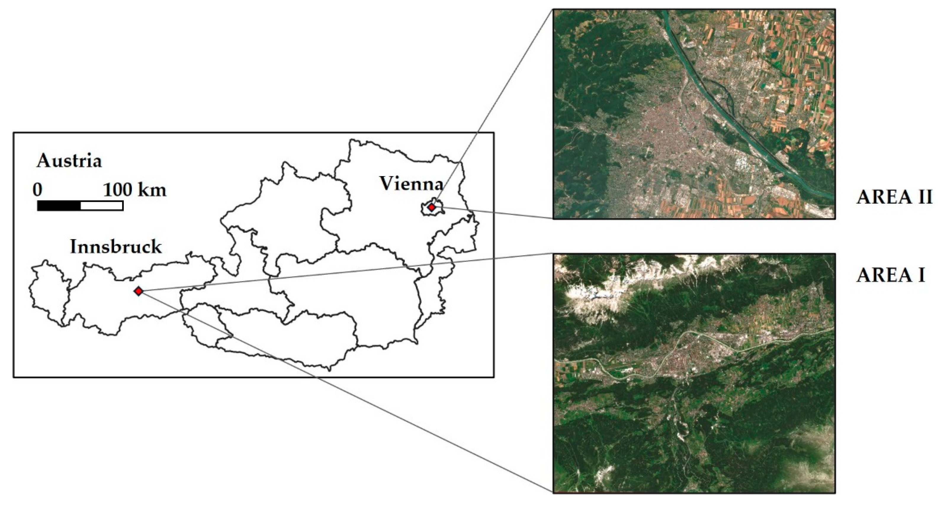
Figure 2.
Overview of the datasets used in the training, shown for AREA I. The datasets are displayed in their native resolution. (a) ECOSTRESS land surface temperature in C°, after masking by the QC layer (date and time of observation: 13.06.2023, 12:40:05, resolution 70 m). Data gaps due to clouds and instrument artifacts are visible. (b) INCA air temperature in C° (date and time of observation: 13.06.2023, 13:00:00, resolution 1 km). The image represents the closest INCA observation to the ECOSTRESS observation shown in (a). (c) Sentinel-2 band B04 reflectance (date and time of observation: 15.07.2023, 10:16:01, resolution 10 m). The image represents the cloud-free observation with all valid pixels closest to the ECOSTRESS observation shown in (a). (d) Digital elevation model (resolution 25 m). (e) Tree cover density. (f) Water and wetness index. (g) Imperviousness. The datasets (e-g) are from the reference year 2018, and they are shown in 10 m resolution.
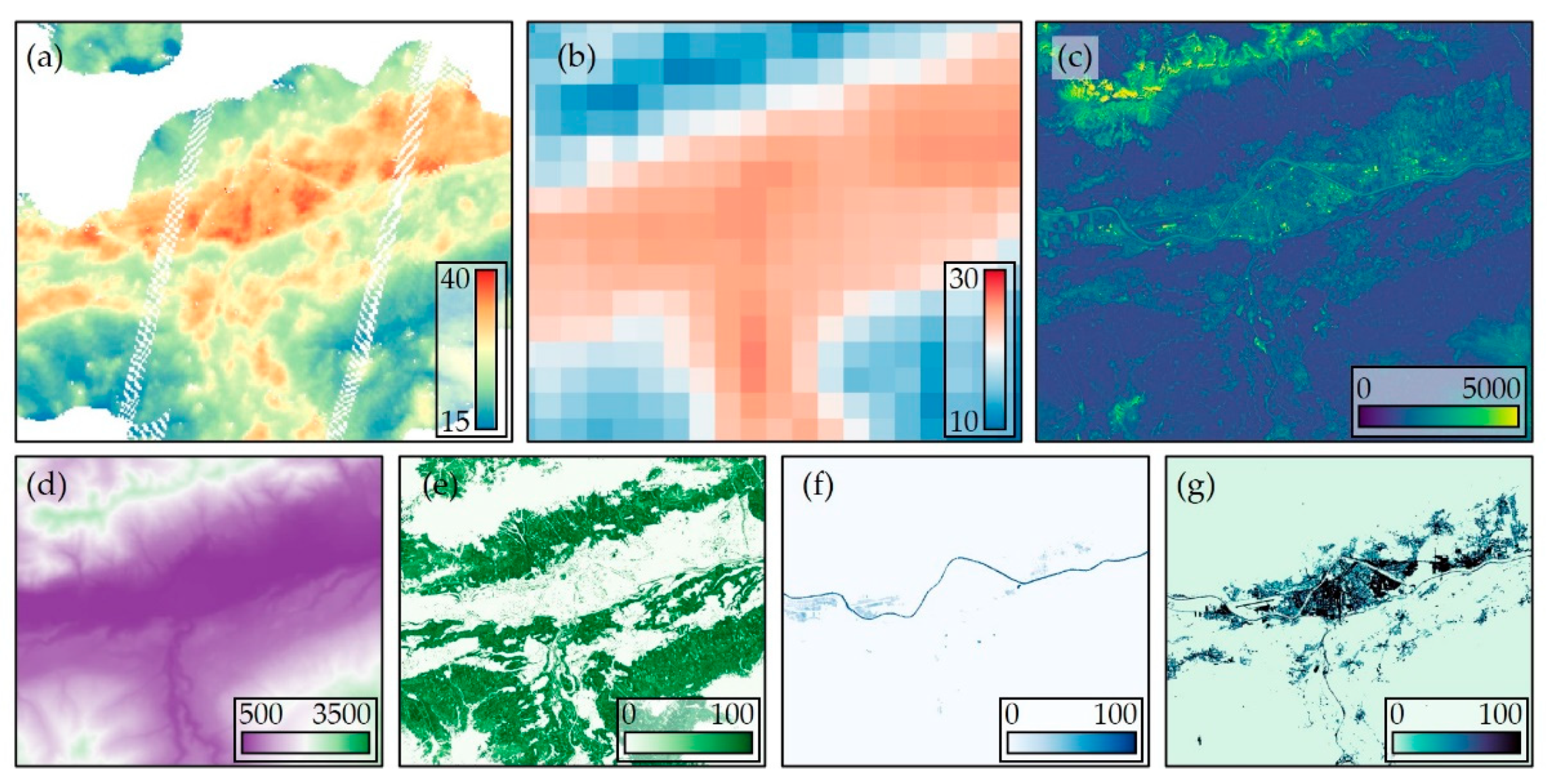
Figure 3.
Scheme of the convolutional neural network architecture used for the land surface temperature predictions.
Figure 3.
Scheme of the convolutional neural network architecture used for the land surface temperature predictions.
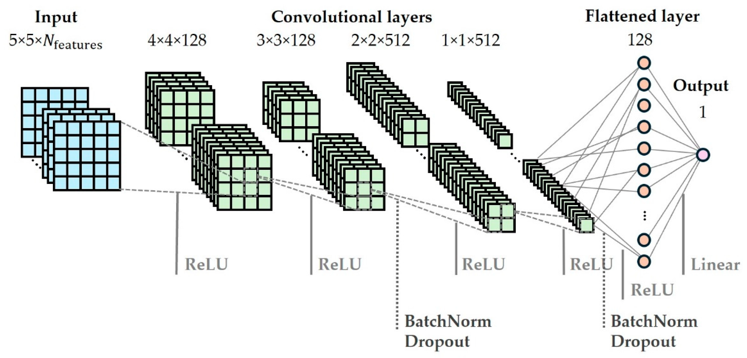
Figure 4.
Comparison between ECOSTRESS measurements and model predictions of land surface temperature (LST) in C°. The images display LST data for two areas of interest, outlined by a bounding box in each image. (a) Masked ECOSTRESS measurement and (b) corresponding model prediction for AREA I. Date and time of observation: 12.06.2022, 13:26:01. (c) Masked ECOSTRESS measurement and (d) corresponding LST prediction over AREA II. Date and time of observation: 04.08.2022, 16:31:34.
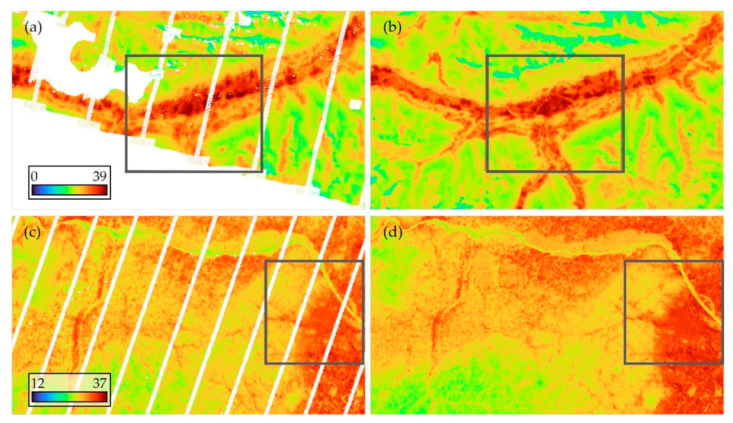
Figure 5.
(a) Close-up of grid artifacts in ECOSTRESS LST observation, shown in grayscale to enhance visibility. (b) The corresponding model prediction corrects the artifacts and increases spatial details. (Location: WGS84 coordinates 48.65398°N, 16.31361°E. Observation date and time: 04.06.2022, 16:39:50).
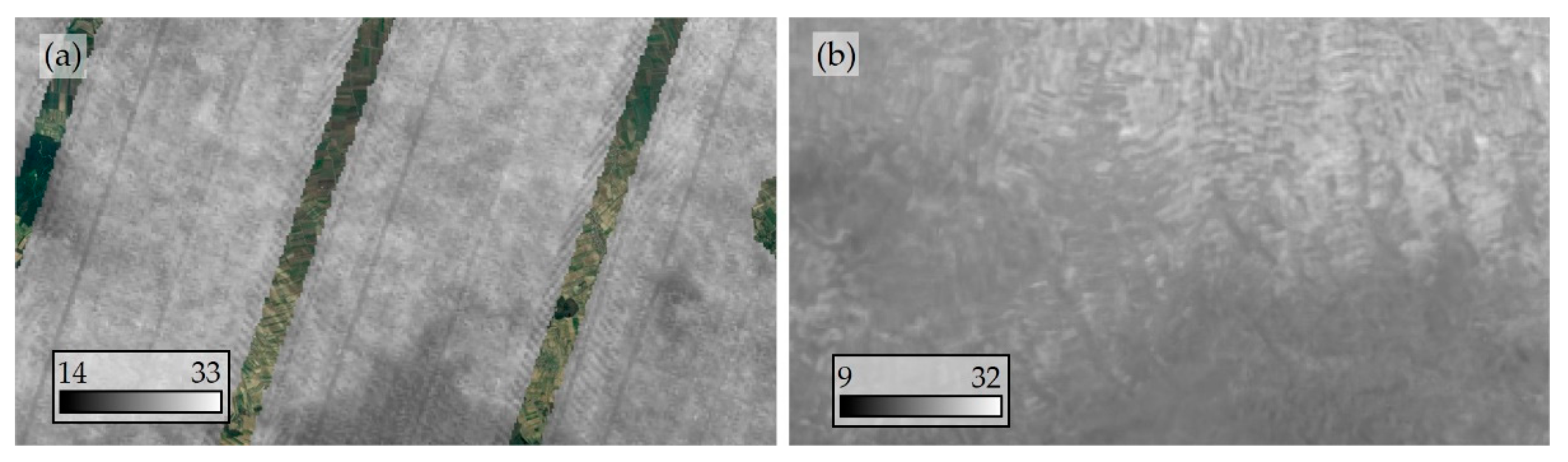
Figure 6.
Histograms for the disjoint (above) and joint (below) distribution of the land surface temperature (LST) of all pixels across all the predictions considered in Table 3. (a-b) Pixelwise results over tile 32TPT. (c-d) Pixelwise results over tile 33UWP. The color bars in the bivariate histograms indicate pixel count.
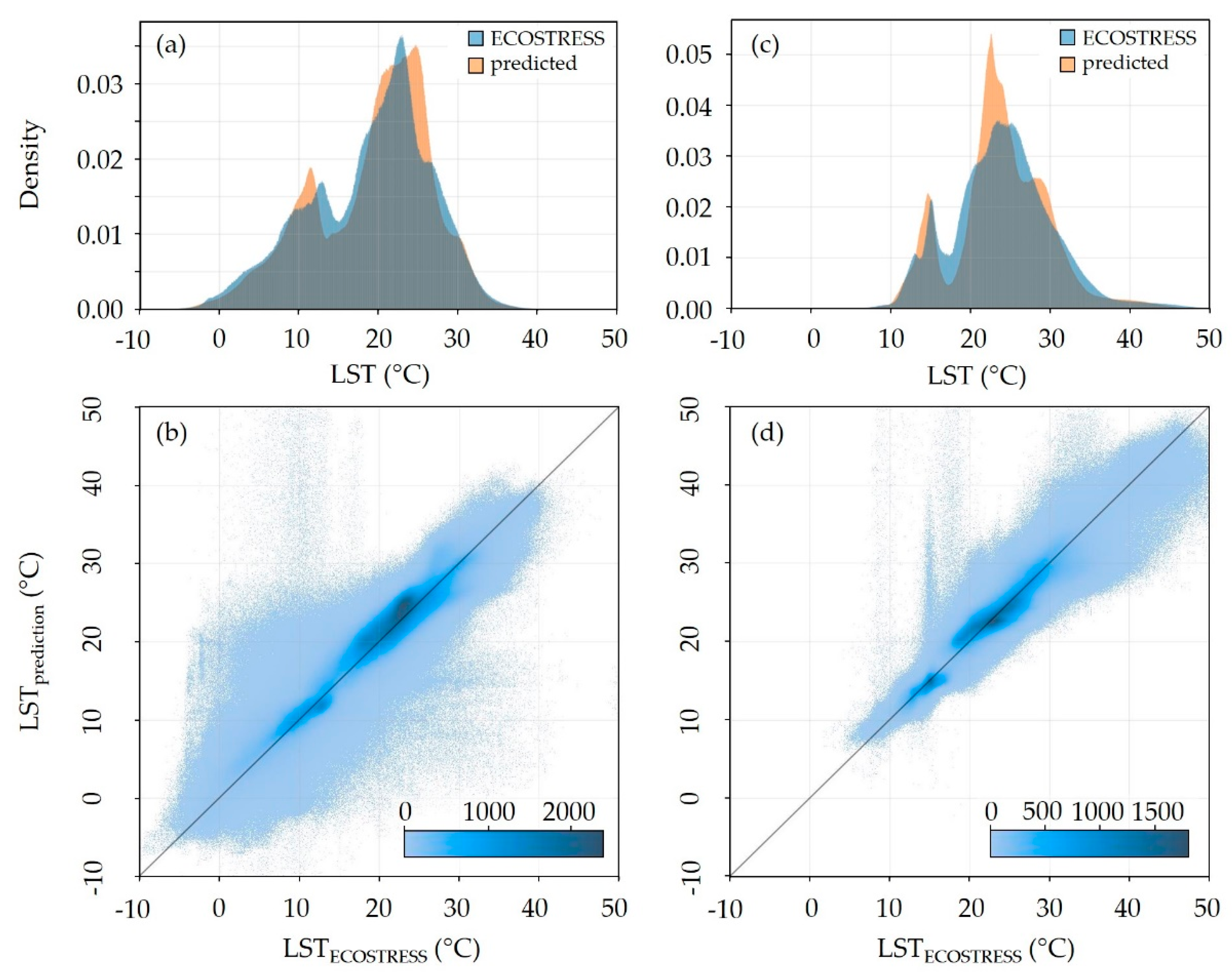
Figure 7.
Histograms for the disjoint (above) and joint (below) distribution of the land surface temperature (LST) of all pixels across all afternoon model predictions considered in Table 3. (a-b) Pixelwise results over tile 32TPT. (c-d) Pixelwise results over tile 33UWP. The color bars in the bivariate histograms indicate pixel count.
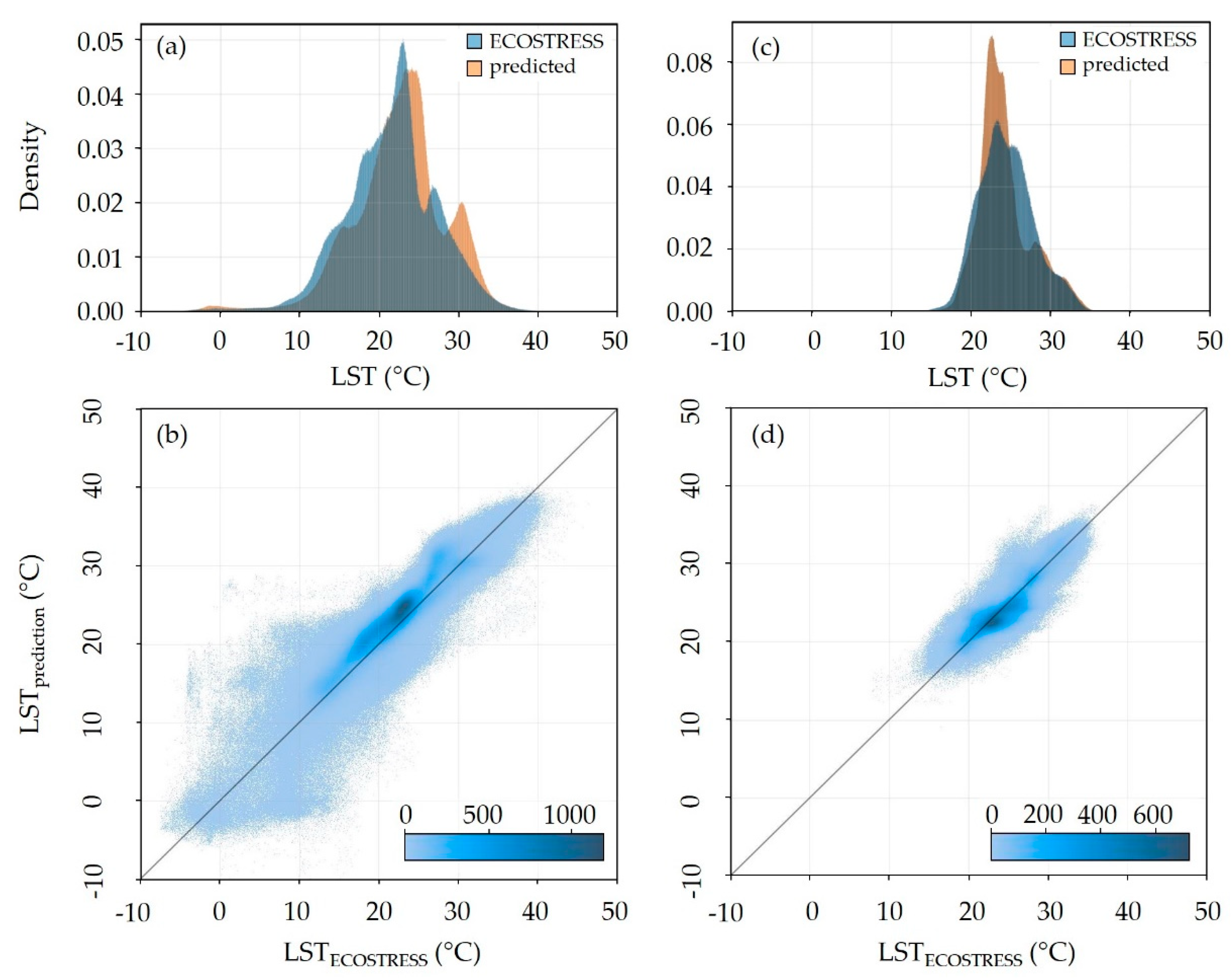
Figure 8.
Examples of data quality issues for ECOSTRESS observations showing land surface temperature in °C. (a) Issues identified in a single observation: missing data due to masking by the ECOSTRESS-QC layer (background image visible); fringe-pattern sensor artifacts that remain even after the QC mask is applied; incorrect georeferencing (cf. position of the river in the ECOSTRESS observation and the background image, the displacement is further accentuated by the double arrow). (Location: WGS84 coordinates: 47.26646°N, 11.38075°E. Observation date and time: 11.06.2022, 14:49:19). (b) Summer observation before masking by the QC layer. A cloud is clearly identifiable by the negative temperature values, inconsistent with the season in which the observation was taken, as well as by the spatial extent which does not follow any spatial features in the area. (Location: WGS84 coordinates: 47.1852°N, 16.8806°E. Observation date and time: 09.07.2022, 03:02:29). (c) The same observation as in (b) after masking by the QC layer, demonstrating that the cloud was not sufficiently masked.
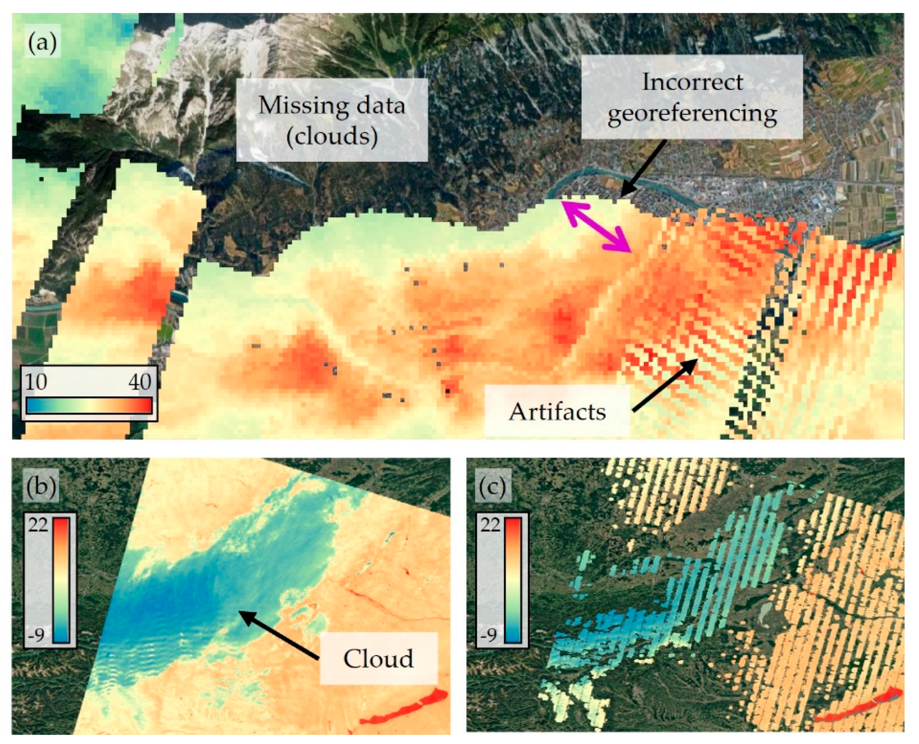

Table 1.
Summary of the datasets used in this study.
| Dataset | Source | Resolution | Considered parameters |
|---|---|---|---|
| ECOSTRESS-LSTE | ECOSTRESS | 70 m | Land surface temperature, quality control |
| INCA | ZAMG, Austria | 1 km | Air temperature at 2 m, relative humidity at 2 m, global radiation, wind speed |
| Sentinel-2 | Sentinel-2 mission | 10/20 m | Bands B2, B3, B4, B8, B11, B12 |
| EU-DEM | Copernicus Land Monitoring Service | 25 m | Elevation, aspect, slope |
| Land cover | Copernicus Land Monitoring Service | 10 m | Tree cover density, water and wetness index, imperviousness |
Table 2.
Summary of the convolutional neural network architecture and hyperparameters.
| input layer | size: 5×5×15 |
| convolutional layers | kernel size: 2×2; stride: 1×1; filters: 128 (layers 1 and 2), 512 (layers 3 and 4) |
| dense layer | size: 128 |
| activation functions | rectified linear unit (‘relu’), for the final layer ‘linear’ |
| Optimizer | adam (with inverse time decay); learning rate schedule: initial_lr=0.001, decay_rate=1, steps=1000×number_samples/batch_size |
| loss function | mean absolute error |
| number of epochs | 50 |
| batch size | 512 |
| train/validation split | 80:20 |
| dropout rate | 0.1 |
Table 3.
Individual and ensemble statistics for the error distributions of 22 model predictions on tile 32TPT and 33UWP. Only the 4 best and 4 worst predictions are shown, based on the mean absolute error (MAE). The predictions are made on ECOSTRESS observations unseen during training, with the date and time of each observation shown in the “date and time” column. The "valid" column indicates the fraction of valid pixels in the ECOSTRESS image (determined by the ECOSTRESS QC mask) for which the statistics is calculated. The “hour range” column indicates the hour range limits for the data used to train the model from which the respective prediction was derived. All metrics are shown in °C, except which is dimensionless.
| 32TPT | ||||||||||||
| date and time | hour range | MAE | ME | r2 | min | max | 10p | 15p | 85p | 90p | std | valid |
| 16.8.2023, 11:38:45 | 11:00-15:00 | 1.01 | 0.0 | 0.81 | -24.32 | 30.05 | -1.49 | -1.18 | 0.93 | 1.28 | 1.79 | 0.59 |
| 4.8.2022, 13:17:00 | 13:00-19:00 | 1.44 | -0.99 | 0.66 | -12.5 | 27.14 | -2.88 | -2.48 | 0.42 | 0.76 | 1.62 | 0.27 |
| 13.6.2023, 12:40:05 | 11:00-15:00 | 1.56 | -0.02 | 0.78 | -12.2 | 25.62 | -2.52 | -1.96 | 1.81 | 2.31 | 2.15 | 0.48 |
| 21.8.2022, 05:57:47 | 04:00-11:00 | 1.6 | 0.51 | 0.68 | -13.92 | 50.95 | -1.78 | -1.32 | 2.39 | 3.06 | 2.16 | 0.77 |
| 8.6.2023, 15:08:57 | 13:00-19:00 | 2.73 | -1.35 | 0.79 | -17.65 | 21.07 | -5.64 | -4.85 | 1.67 | 2.34 | 3.28 | 0.13 |
| 22.7.2023, 17:13:37 | 00:00-23:00 | 2.97 | 2.08 | -0.27 | -27.62 | 98.1 | -1.35 | -0.43 | 3.83 | 4.56 | 4.68 | 0.3 |
| 19.8.2023, 06:01:12 | 03:00-07:00 | 3.09 | 0.02 | 0.23 | -49.21 | 41.42 | -4.16 | -3.22 | 3.89 | 4.74 | 4.49 | 0.21 |
| 19.8.2023, 06:01:12 | 00:00-23:00 | 3.67 | -2.35 | -0.02 | -50.53 | 51.82 | -7.02 | -5.83 | 1.59 | 2.53 | 4.62 | 0.21 |
| ensemble statistics | - | 1.93 | 0.36 | 0.87 | -50.53 | 98.1 | -2.59 | -1.94 | 2.62 | 3.16 | 2.71 | 0.54 |
| 33UWP | ||||||||||||
| date and time | hour range | MAE | ME | r2 | min | max | 10p | 15p | 85p | 90p | std | valid |
| 2.7.2022, 5:26:25 | 00:00-23:00 | 0.85 | -0.14 | 0.46 | -6.81 | 28.6 | -1.43 | -1.16 | 0.74 | 1.04 | 1.38 | 0.62 |
| 2.7.2022, 5:26:25 | 03:00-07:00 | 0.98 | -0.46 | 0.49 | -5.69 | 25.87 | -1.83 | -1.58 | 0.65 | 0.92 | 1.27 | 0.62 |
| 15.8.2023, 07:36:45 | 04:00-11:00 | 1.1 | 0.0 | 0.69 | -7.39 | 8.05 | -1.77 | -1.4 | 1.38 | 1.74 | 1.43 | 0.66 |
| 2.7.2022, 5:26:25 | 04:00-11:00 | 1.1 | 0.03 | -0.13 | -16.65 | 56.41 | -1.65 | -1.37 | 1.23 | 1.56 | 2.01 | 0.62 |
| 16.8.2022, 11:38:39 | 00:00-23:00 | 2.18 | -0.72 | 0.81 | -20.24 | 17.37 | -4.45 | -3.42 | 1.85 | 2.41 | 2.97 | 0.41 |
| 12.8.2023, 13:13:33 | 07:00-11:00 | 2.26 | -0.65 | -0.15 | -13.32 | 62.62 | -3.9 | -3.35 | 1.98 | 3.06 | 2.84 | 0.24 |
| 18.6.2023, 10:13:08 | 00:00-23:00 | 2.55 | -2.14 | 0.4 | -17.4 | 7.81 | -5.7 | -4.88 | 0.27 | 0.72 | 2.59 | 0.53 |
| 18.6.2023, 10:13:08 | 00:00-23:00 | 2.61 | -2.39 | 0.4 | -17.34 | 62.68 | -5.59 | -4.81 | -0.21 | 0.33 | 2.33 | 0.53 |
| ensemble statistics | - | 1.6 | -0.15 | 0.87 | -33.14 | 135.46 | -2.68 | -2.08 | 1.78 | 2.27 | 2.22 | 0.59 |
Table 4.
Ensemble statistics for the predictions of Table 3 that were derived from a full-day model or an afternoon model, grouped by model type and tile.
Table 4.
Ensemble statistics for the predictions of Table 3 that were derived from a full-day model or an afternoon model, grouped by model type and tile.
| Model | MAE | ME | r2 | min | max | 10p | 15p | 85p | 90p | std | valid |
|---|---|---|---|---|---|---|---|---|---|---|---|
| 32TPT, full day | 2.16 | -0.04 | 0.82 | -50.53 | 98.1 | -3.41 | -2.69 | 2.48 | 3.04 | 3.09 | 0.55 |
| 32TPT, afternoon | 1.96 | 1.06 | 0.81 | -27.3 | 27.14 | -1.56 | -0.92 | 3.02 | 3.47 | 2.29 | 0.48 |
| 33UWP, full day | 1.79 | -0.25 | 0.85 | -33.14 | 135.46 | -3.17 | -2.48 | 1.86 | 2.38 | 2.51 | 0.58 |
| 33UWP, afternoon | 1.39 | -0.19 | 0.73 | -9.71 | 10.44 | -2.4 | -1.94 | 1.58 | 2.06 | 1.77 | 0.61 |
Table 5.
Ensemble statistics for extrapolating morning predictions from afternoon models.
| Model | MAE | r2 | ME | min | max | 10p | 15p | 85p | 90p | std | valid |
| 32TPT, extrapolating predictions | 3.12 | 0.72 | -0.35 | -52.81 | 56.51 | -5.41 | -4.28 | 3.42 | 4.33 | 4.14 | 0.55 |
| 33UWP, extrapolating predictions | 2.96 | 0.64 | 0.28 | -46.14 | 30.37 | -4.67 | -3.48 | 3.92 | 4.57 | 3.8 | 0.61 |
Disclaimer/Publisher’s Note: The statements, opinions and data contained in all publications are solely those of the individual author(s) and contributor(s) and not of MDPI and/or the editor(s). MDPI and/or the editor(s) disclaim responsibility for any injury to people or property resulting from any ideas, methods, instructions or products referred to in the content. |
© 2024 by the authors. Licensee MDPI, Basel, Switzerland. This article is an open access article distributed under the terms and conditions of the Creative Commons Attribution (CC BY) license (http://creativecommons.org/licenses/by/4.0/).
Copyright: This open access article is published under a Creative Commons CC BY 4.0 license, which permit the free download, distribution, and reuse, provided that the author and preprint are cited in any reuse.


