
Submitted:
09 November 2024
Posted:
13 November 2024
You are already at the latest version
Abstract
Accurate sales forecasting is essential for optimizing resource allocation, managing inventory, and maximizing profit in competitive markets. Machine learning models are increasingly used to develop reliable sales forecasting systems due to their advanced capabilities in handling complex data patterns. This study introduces a novel hybrid approach that combines the Artificial Bee Colony (ABC) and Fire Hawk Optimizer (FHO) algorithms, specifically designed to enhance hyperparameter optimization in machine learning-based forecasting models. Leveraging the strengths of these two metaheuristic algorithms, the hybrid method enhances the predictive accuracy and robustness of models, with a focus on optimizing the hyperparameters of XGBoost for forecasting tasks. Evaluations across three distinct datasets demonstrate that the hybrid model consistently outperforms standalone algorithms, including Genetic Algorithm (GA), Artificial Rabbits Optimization (ARO), White Shark Optimizer (WSO), ABC, and FHO, the latter being applied for the first time to hyperparameter optimization. The superior performance of the hybrid model is confirmed through RMSE, MAPE, and statistical tests, marking a significant advancement in sales forecasting and providing a reliable, effective solution for refining predictive models to support business decision-making.
Keywords:
extreme gradient boosting
; Machine Learning Algorithm
; Forecasting Model
; Metaheuristic Algorithms
; Hyperparameter tuning
; Hybrid Metaheuristic
1. Introduction
Sales forecasting is essential for businesses to manage inventory efficiently, optimize resource allocation, and maintain profitability. It allows companies to anticipate demand, avoid overstocking or understocking, and minimize waste. Accurate sales forecasts are particularly critical in industries with volatile demand patterns or seasonal variations, enabling informed decisions in production, staffing, and logistics. By adopting advanced forecasting methods, businesses can better meet market demands, enhance customer satisfaction, and remain competitive in a rapidly changing environment.
Machine learning has become a powerful tool in sales forecasting, significantly improving prediction accuracy in complex and dynamic environments. It has been widely applied to manage the nonlinear relationships inherent in large datasets, offering superior forecasting outcomes, particularly for seasonal or promotional sales (Huber & Stuckenschmidt, 2020). Among machine learning algorithms, XGBoost has consistently outperformed models such as random forests and neural networks across various forecasting tasks (Ben Jabeur et al., 2024). In retail demand forecasting, XGBoost has demonstrated its superiority, achieving higher accuracy and reducing prediction error compared to traditional models like ARIMA (Zhang et al., 2021; Massaro et al., 2021). Studies in the retail and e-commerce sectors further validate XGBoost’s reliability in handling large-scale forecasting challenges (Panarese et al., 2021).
Hyperparameter optimization is crucial in improving the performance of machine learning models by enhancing their ability to generalize to unseen data. Proper selection of hyperparameters can significantly impact model accuracy, and tuning these parameters ensures the model reaches its optimal potential. Without adequate tuning, even high-performing models may fail to reach their full potential, leading to incorrect assessments of their effectiveness (Arnold et al., 2024). Systematic hyperparameter tuning is essential for robust and reliable machine learning applications, particularly in complex forecasting tasks. Advanced optimization techniques, such as genetic algorithms and swarm intelligence, further enhance hyperparameter tuning by reducing computational costs and increasing efficiency in handling complex models (Ali et al., 2023).
Metaheuristic algorithms have emerged as effective tools for hyperparameter optimization, offering superior performance over traditional methods like grid search by efficiently exploring large and complex search spaces. In recent years, the use of metaheuristic algorithms for hyperparameter optimization has significantly improved the performance of forecasting models across various domains. For instance, solar energy forecasting has benefited from metaheuristic-based approaches like genetic algorithms (GA), which have enhanced the accuracy of long short-term memory (LSTM) networks by optimizing their hyperparameters, achieving substantial reductions in forecasting error (Dhake et al., 2023). In electricity load forecasting, combining support vector machines (SVM) with adaptive differential evolution (ADE) for hyperparameter tuning has resulted in high accuracy and better convergence rates (Zulfiqar et al., 2022). In combinatorial optimization problems, ABC has proven its versatility, achieving competitive results in areas like assembly line balancing and bioinformatics, further validating its robustness and applicability across multiple domains (Kaya et al., 2022). Moreover, Grey Wolf Optimization (GWO) has demonstrated its effectiveness in hyperparameter optimization tasks, enhancing model accuracy and minimizing loss, particularly in complex machine learning models like CNNs (Mohakud & Dash, 2021). Metaheuristic algorithms like genetic algorithms have also proven effective in temperature forecasting, enhancing the performance of LSTM networks for long-term meteorological predictions (Tran et al., 2020). The recently developed Fire Hawk Optimizer (FHO) further exemplifies this potential, effectively balancing exploration and exploitation in the optimization process (Hosseinzadeh et al., 2023; Abd Elaziz et al., 2023).
While individual metaheuristic algorithms show great potential, hybridizing them can yield even better results. Hybrid algorithms combine the strengths of different metaheuristics to overcome their individual limitations, such as getting stuck in local optima or slow convergence. For example, hybridizing the White Shark Optimizer (WSO) with Artificial Rabbits Optimization (ARO) has achieved superior accuracy in photovoltaic parameter extraction by combining WSO’s global search capabilities with ARO’s local search efficiency (Çetinbaş et al., 2023). Similarly, hybrid approaches that integrate ant colony optimization (ACO) with other algorithms, such as the Reptile Search Algorithm (RSA), have demonstrated improved performance in forecasting tasks by enhancing the balance between exploration and exploitation (Al-Shourbaji et al., 2022). The Artificial Bee Colony (ABC) algorithm has been effectively applied to feature selection and optimization tasks, showing superior performance in selecting relevant features and enhancing classification accuracy when combined with other metaheuristics (Bindu & Sabu, 2020). The integration of hybrid metaheuristics has shown superior performance, especially in complex optimization scenarios where a single algorithm might fall short (Abd Elaziz et al., 2023).
After a thorough examination of the literature, we identified key areas where further development remains possible in the field of hyperparameter optimization. In response, this study proposes a novel approach by hybridizing the Artificial Bee Colony (ABC) algorithm with the Fire Hawk Optimizer (FHO), leveraging the strengths of each to enhance the performance of machine learning models in sales forecasting. Notably, this is among the first applications of FHO as a standalone algorithm for hyperparameter optimization in XGBoost, specifically within a sales forecasting context. Our research aims to develop robust, generalizable models by testing the hybrid approach on three distinct open-source datasets, ensuring the models' adaptability across various forecasting scenarios. To validate our approach, we rigorously evaluated the proposed hybrid model using statistical tests, which confirmed its effectiveness and robustness, contributing not only to the academic field but also providing a practical, scalable solution for real-world forecasting tasks.
The remainder of this article is structured as follows: Section 2 outlines the methodology, detailing the hybrid metaheuristic approach used for hyperparameter optimization. In Section 3, we present the case study, applying the proposed algorithms to three open-source sales forecasting datasets. Section 4 discusses the experimental results and performance analysis of the hybrid models. Finally, Section 5 concludes the paper by summarizing the key findings and suggesting future research directions.
2. Methodology
2.1. XGBoost Algorithm
XGBoost, built on the Gradient Boosting Decision Tree (GBDT) framework, excels in both classification and regression tasks by sequentially boosting weak learners to minimize error. One of its standout features is the inclusion of regularization in its objective function, which effectively reduces overfitting by balancing accuracy and model complexity. This balance allows XGBoost to generalize well to unseen data, making it particularly suitable for large datasets with complex, nonlinear relationships. The algorithm’s capability to tune hyperparameters and handle missing data efficiently contributes to its high performance across various forecasting tasks (Abbasimehr et al., 2023).
XGBoost operates by sequentially building decision trees, with each new tree focusing on correcting errors made by the previous ones. This is achieved through gradient boosting, a process that optimizes the objective function by minimizing loss and incorporating regularization terms to avoid overfitting. Specifically, the algorithm computes the negative gradient (representing the error) and uses it to create new trees that target these errors. The result is a robust predictive model composed of an ensemble of weaker learners (Deng et al., 2022).
2.2. Genetic Algorithm
The Genetic Algorithm (GA) is an optimization method inspired by principles of natural selection and evolution. Initially introduced by J.H. Holland in 1992, GA simulates "survival of the fittest" by working with a population of potential solutions, represented as chromosomes, which evolve over several generations to find the optimal result. Key processes in GA include encoding chromosomes, selecting candidates based on their fitness, performing crossover to blend genetic traits from two parent solutions, and applying mutation to introduce random variations. This mechanism allows GA to effectively search extensive solution spaces and identify global optima, making it especially useful for complex optimization problems. For an in-depth review, refer to Katoch et al. (2021).
2.3. Grey Wolf Optimizer
The Grey Wolf Optimizer (GWO) is a metaheuristic algorithm inspired by the natural social hierarchy and hunting behavior of grey wolves, introduced by Mirjalili in 2014. GWO simulates a leadership structure by categorizing the population into four ranks: alpha, beta, delta, and omega, with the alpha wolf leading the pack, followed by the beta and delta wolves. The wolves work together to encircle, pursue, and capture prey, symbolizing the optimization process. GWO strikes a balance between exploration and exploitation through parameters that adjust the wolves' positions with each iteration, enabling it to effectively search and refine solutions within the search space. Its simplicity, lack of complex parameters, and reliable performance have made GWO popular for solving optimization problems across various fields, including engineering, bioinformatics, and robotics (Makhadmeh et al., 2023).
2.4. White Shark Optimizer
The White Shark Optimizer (WSO) is a metaheuristic algorithm inspired by the hunting behavior of white sharks, introduced by Braik et al. in 2022. The algorithm simulates the sharks' remarkable ability to track prey over long distances using their heightened senses, adjusting their movements strategically to locate and capture targets. In optimization, search agents (representing sharks) adaptively move towards optimal solutions while periodically exploring new areas of the search space to avoid getting stuck in local optima. By balancing exploration and exploitation, WSO has demonstrated effectiveness in solving complex optimization problems, making it suitable for both constrained and unconstrained scenarios (Braik et al., 2022).
2.5. Artificial Rabbits Optimization
The Artificial Rabbits Optimization (ARO) algorithm is a bio-inspired metaheuristic that mimics the survival strategies of rabbits in nature, including detour foraging and random hiding. In detour foraging, rabbits search for food away from their nests, which enhances exploration, allowing the algorithm to avoid local optima. On the other hand, random hiding helps exploit nearby solutions by encouraging rabbits to choose randomly among several burrows for safety, thus balancing exploitation. The algorithm dynamically shifts between these two strategies as the "energy" of the rabbits diminishes over time, transitioning from exploration in the early stages to exploitation in the later iterations. For further details on the ARO algorithm, please refer to the work by Wang et al. (2022)
2.6. Artificial Bee Colony
The Artificial Bee Colony (ABC) algorithm, introduced by Karaboga in 2005, is a nature-inspired optimization technique modeled after the foraging behavior of honeybees. It mimics how bees search for food sources, with three types of bees: employed, onlooker, and scout bees. Employed bees exploit known food sources, while onlooker bees select food sources based on shared information from employed bees. Scout bees search for new food sources when existing ones are exhausted. This process enables the algorithm to balance exploration and exploitation efficiently, making it particularly effective for solving complex optimization problems. The ABC algorithm has been successfully applied to a wide range of optimization tasks, such as engineering, telecommunications, and data mining, due to its simplicity and robust performance (Kaya et al., 2022).
The algorithm begins by initializing a population of potential solutions, represented by the locations of food sources. Each employed bee is associated with a food source, and the quality of the solution is measured by the amount of nectar (fitness) at that location. Employed bees explore the neighborhood of their associated food source to find better solutions. Meanwhile, onlooker bees assess the quality of the food sources shared by the employed bees through a waggle dance, selecting solutions probabilistically based on their fitness. Scout bees search for new food sources by exploring unexplored regions of the search space when current sources are exhausted or abandoned (Jahangir & Rezazadeh Eidgahee, 2021).
| 1. Initialize parameters (number of food sources, employed bees, onlooker bees, and scout bees).. |
| 2. Randomly generate an initial population of food sources (possible solutions). |
| 3. SEvaluate the fitness of each food source. |
| 4. Repeat until the termination condition is met: |
| 4.1 For each employed bee: |
| - Explore the neighborhood of the associated food source to discover new solutions. |
| - If a new solution is better than the current one, replace the old solution with the new one. |
| 4.2 Calculate the probability of each food source based on its fitness. |
| 4.3 For each onlooker bee: |
| - Select a food source probabilistically based on fitness. |
| - Explore the neighborhood of the chosen food source. |
| - If a new solution is better, update the food source. |
| 4.4 If a food source has not improved for a predetermined number of cycles: |
| - Abandon the food source. |
| - Send a scout bee to explore a new random location. |
| 5. Memorize the best solution found so far. |
| 6. End. |
2.7. Fire Hawk Optimizer
Fire Hawk Optimizer (FHO) is a metaheuristic algorithm inspired by the behavior of fire hawks, which intentionally spread fires to flush out prey. This optimization method mimics the process by which fire hawks identify and target prey, using exploration (setting fires in new areas) and exploitation (capturing prey in known areas). FHO uses position updates based on the prey's movement and safe zones, balancing exploration and exploitation to avoid local optima and reach the global optimum efficiently. It has been proven effective in solving complex optimization problems across various domains due to its quick convergence and robust search strategies (Azizi et al., 2022).
| 1. Initialization of the population: Initialize a population of fire hawks and prey (possible solutions). |
| 2. Re-reading and evaluation: Evaluate the fitness of each prey (solution). |
| 3. Sending the fire hawks to hunt prey: |
| - Fire hawks move towards the prey based on their fitness (distance from the prey). |
| -If a fire hawk finds a better prey, it updates its position to that new prey. |
| 4. Sending other fire hawks to improve exploration: |
| -Fire hawks that are far from the best prey are sent to explore new regions of the search space. |
| -Fire hawks adapt their positions to explore areas with high potential. |
| 5. Sending the scout fire hawks to discover new prey: |
| -If a fire hawk doesn't find better prey within a certain number of moves, it is repositioned to a new location. |
| -Scout fire hawks are used to explore unknown areas to avoid local optima. |
| 6. Memorizing the best prey found so far and updating the position of the fire hawks accordingly. |
| 7. Repeating the steps until the termination condition is met. |
2.8. Hybrid ABC-FHO Algorithm
The hybridization of the Artificial Bee Colony (ABC) and Fire Hawk Optimizer (FHO) leverages the strengths of both algorithms for a balanced and efficient optimization process. ABC excels in balancing exploration and exploitation through its employed, onlooker, and scout bee phases, but it can sometimes struggle with convergence speed, particularly in complex search spaces. In contrast, FHO adapts its search strategy based on the distance from the best solution, performing either global or local searches. This hybrid approach addresses the limitations of each individual algorithm, improving overall performance.
The process begins with ABC’s employed bees, where each agent (bee) is randomly initialized within the search space and explores its local neighborhood. The new solution for each agent is generated using:
where ϕ is a random perturbation, is the current solution, and is a randomly chosen neighbor. This broad exploration helps avoid local optima, but it is stochastic in nature, requiring more refinement in later stages.
The onlooker bee phase follows, refining the search by selecting solutions probabilistically based on fitness:
This step shifts the focus towards exploitation, giving higher attention to better solutions. However, this can lead to over-exploitation if not balanced, making FHO a valuable addition at this stage.
FHO is introduced to perform adaptive searches. If an agent is far from the best solution, it performs a global search:
where α is a larger step size for exploration. If the agent is close to the best solution, a local search with a smaller step size is used for fine-tuning:
This adaptive behavior ensures the balance between exploration and exploitation, effectively addressing ABC’s tendency to over-exploit certain regions.
To maintain diversity and avoid stagnation, ABC’s scout bee phase replaces agents that have not improved after a set number of iterations with new, randomly generated solutions. This step ensures continued exploration across the search space, preventing the algorithm from converging prematurely to suboptimal solutions.
By combining ABC’s broad exploration with FHO’s adaptive refinement, the hybrid approach accelerates convergence while reducing the likelihood of getting stuck in local optima. This results in a more robust and efficient optimization algorithm, particularly well-suited for complex and dynamic search spaces.
| 1. Initialize population of agents randomly in the search space. |
| 2. Evaluate the fitness of all agents. |
| 3. Repeat until maximum iterations are reached: |
| 3.1 ABC: Employed Bee Phase |
| - For each agent: |
| - Generate a new solution by modifying the current agent’s position. |
| - If the new solution is better, update the agent's position and reset its trial counter. |
| - If not, increase the trial counter for that agent. |
| 3.2 ABC: Onlooker Bee Phase |
| - Select agents probabilistically based on their fitness. |
| - Generate new solutions as in the employed bee phase. |
| 3.3 FHO: Fire Hawk Search |
| - For each agent: |
| - Determine whether to perform a global or local search based on the distance to the best solution. |
| - If performing a global search, make larger steps in the search space. |
| - If performing a local search, make smaller steps for fine-tuning. |
| 3.4 ABC: Scout Bee Phase |
| - Replace agents that have not improved after a certain number of attempts with new random solutions. |
| 4. Return the best solution and its fitness. |
2.9.1. Statistical Metrics
2.9.1.1. Shapiro-Wilk
The Shapiro-Wilk test, introduced by Shapiro and Wilk in 1965, is a widely used goodness-of-fit test that assesses whether a dataset follows a normal distribution. The test computes a statistic based on the ordered sample values, comparing them to corresponding expected values from a normal distribution. If the computed statistic deviates significantly from the expected distribution, the null hypothesis of normality is rejected. This test is particularly powerful for small to medium-sized datasets, making it a popular choice in statistical analyses (Shapiro & Wilk, 1965).
For more detailed applications and extensions of the test, particularly in the presence of regression and scale, refer to studies such as Jurečková & Picek (2007), which explore adaptations of the test under different statistical conditions.
2.9.1.2. Mann-Whitney U Test
The Mann-Whitney U test is a non-parametric statistical test used to compare differences between two independent groups. It is often used as an alternative to the t-test when the data do not meet the assumptions of normality. The Mann-Whitney U test evaluates whether one group tends to have larger values than the other without assuming a normal distribution of the data. This test ranks the combined data of both groups and then compares the sum of ranks between the groups to determine whether the distributions differ significantly. The null hypothesis (H0) assumes there is no difference between the two groups in terms of their distributions, while the alternative hypothesis (Ha) suggests that the distributions are different. The test is useful in various fields, including biology, social sciences, and medical research, where the assumptions of parametric tests may not be satisfied (MacFarland & Yates, 2016)
3. Case Study
This section outlines the experiments conducted to evaluate the performance of GA, ARO, WSO, standalone ABC, standalone FHO, and the hybrid ABC-FHO in sales forecasting. Their performance is compared across three different sales datasets, which include a variety of features and instances. Figure 3.1 to 3.3 present sales graphs for each dataset.
Figure 3.
1. Dataset 1 Sales Graph.
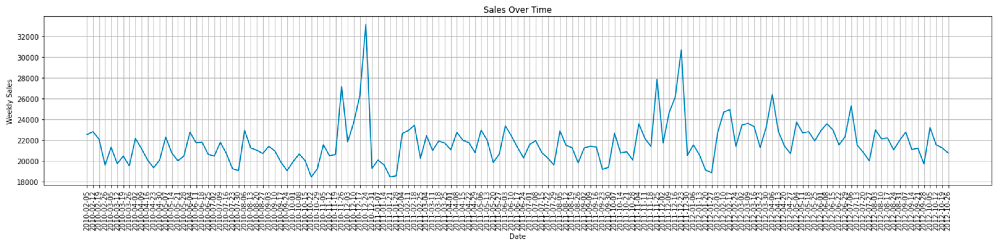
Figure 3.
2. Dataset 2 Sales Graph.
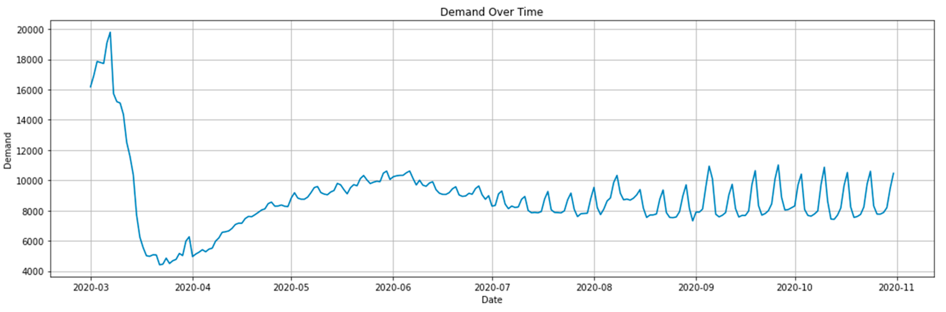
Figure 3.
3. Dataset 3 Sales Graph.
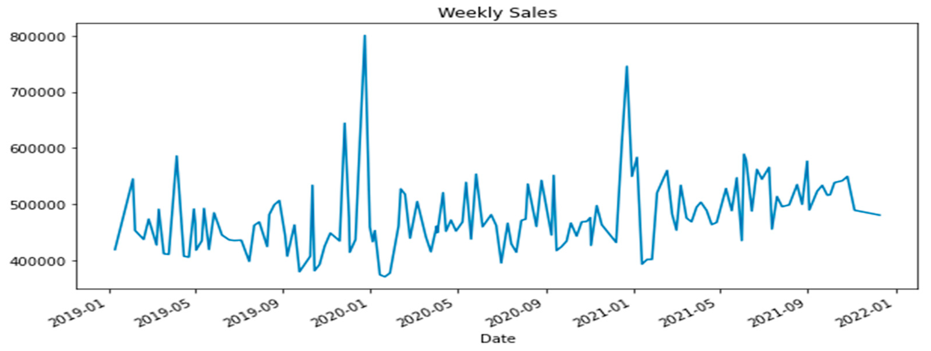
The datasets in this study, illustrated in Figure 3.1 to 3.3 and summarized in Table 3.1, capture a range of sales dynamics with varying temporal patterns, demand fluctuations, and feature complexities. This diversity enables a rigorous assessment of the hybrid ABC-FHO model’s performance across distinct sales environments.

Table 3.
1. The datasets used in the experiments.
| Dataset | Source | No. of Instances | No. of Features |
|---|---|---|---|
| Dataset 1 | https://github.com/ashfarhangi/COVID-19/ (accessed on 8 October 2024) | 30264 | 13 |
| Dataset 2 | https://www.kaggle.com/datasets/aslanahmedov/walmart-sales-forecast (accessed on 8 October 2024) | 8190 | 12 |
| Dataset 3 | https://data.world/revanthkrishnaa/amazon-uk-sales-forecasting-2018-2021/workspace/project-summary (accessed on 8 October 2024) | 8661 | 21 |
3.1. Experimental Setup
All experiments were implemented in Python and executed on a 3.13 GHz PC with 16 GB RAM, running Windows 10. The performance of the proposed algorithms was validated by conducting experiments using publicly available sales datasets. The characteristics of these datasets are outlined in Table 1, including the number of features, instances, and the dataset sources. To standardize results, each dataset was preprocessed to handle any missing or outlier data before training, ensuring model consistency across all trials. Each dataset was randomly divided into 80% for training and 20% for testing, with a 5-fold cross-validation applied to evaluate the model's performance. To ensure reproducibility, a fixed random seed of 42 was used for all experiments.
3.2. Parameter Settings
The GA, ARO, WSO, standalone ABC, standalone FHO, and hybrid ABC-FHO approaches are evaluated alongside well-known metaheuristics. Parameter settings play a crucial role in optimizing the performance of these algorithms. For all algorithms, a population size of 10 and a maximum of 30 iterations were selected empirically. Each algorithm is executed independently 10 times to ensure reliable results for statistical testing. Additionally, default parameter settings for each algorithm were determined according to their respective implementations, and they are presented in Table 3.2 below:
Table 3.3 presents the initial range of hyperparameters for the XGBoost algorithm, encompassing a wide range to explore potential configurations. These bounds, including parameters like colsample_bytree, n_estimators, and learning_rate, were designed to allow flexibility in parameter tuning and ensure a comprehensive search of the solution space.
Table 3.
2. Selected parameters of metaheuristic algorithms.
| Algorithm | Parameters |
|---|---|
| GA | Population size = 10, Crossover rate = 0.8, Mutation rate = 0.05 |
| ARO | Exploration factor (α) = 0.1, Exploitation factor (β) = 0.9 |
| WSO | Wormhole probability (WEP) = 0.2, WEP_max = 1, Pmax = 6, WEP_min = 0.3 |
| GWO | a= [0,2] |
| Standalone ABC | Colony size = 10, Limit = 5, Food source = 5 |
| Standalone FHO | Prey attraction (γ) = 0.8, Randomness factor (θ) = 0.3 |
| Hybrid ABC-FHO | Colony size = 10 (ABC), Prey attraction (γ) = 0.8 (FHO), Crossover rate = 0.7 |
Table 3.
3. The lower and upper bounds of hyperparameters of XGBoost.
| Hyperparameters | Lower Bound | Upper Bound | Default Value |
|---|---|---|---|
| colsample_bytree | 0.1 | 1 | 1 |
| n_estimators | 30 | 400 | 100 |
| max_depth | 0 | ∞ | 6 |
| learning_rate | 0.1 | 1 | 0.3 |
| min_child_weight | 0.1 | ∞ | 1 |
| reg_alpha | 0 | ∞ | 0 |
| reg_lambda | 0 | ∞ | 1 |
| subsample | 0 | 1 | 1 |
| num_leaves | 1 | ∞ | 1 |
Table 3.4 shows the refined search range for the hyperparameters used in the case study. This focused range was selected based on initial empirical tests, narrowing down the bounds to values likely to yield optimal model performance while reducing computational demands. This refinement ensures that the optimization process is both efficient and targeted, facilitating robust model tuning within practical time limits.
In this study, we employ the hybrid ABC-FHO approach, along with several comparison algorithms, to optimize these hyperparameters within the search space defined in Table 3.4. By using this comprehensive range, the algorithms can explore a wide search space, aiming to identify the optimal parameter settings that maximize the predictive accuracy of the XGBoost model. This setup allows us to effectively evaluate the performance of the hybrid and comparison algorithms in tuning the model for enhanced forecasting accuracy.
3.3. Evaluation Metrics
In this study, two statistical metrics are employed to assess the accuracy of the forecasting models. These metrics are Mean Absolute Percentage Error (MAPE) and Root Mean Squared Error (RMSE). In the following equations (1,2) N represents the quantity of observations during both the training or testing phases, denotes observed value, represents the prediction and refers to the average of the actual values.
- MAPE calculates the average percentage error between the predicted and actual values, providing a normalized measure of accuracy.
- RMSE measures the square root of the average squared differences between predicted and observed values, which gives more weight to larger errors.
Smaller values for both metrics (MAPE and RMSE) indicate better model performance, as they signify lower prediction error. These metrics were computed for both the training and testing stages to ensure robustness of the forecasting models (Tao et al., 2023; Che et al., 2024).
3.4. Results and Analysis
This subsection presents the performance results of GA, ARO, WSO, standalone ABC, standalone FHO, and hybrid ABC-FHO. The evaluation is based on the performance measurements mentioned previously, with additional analysis of convergence behavior, boxplots, statistical analysis.
3.3.1. Performance Results
The performance of the algorithms across the three sales forecasting datasets is summarized in Table 3.3 to Table 3.6. Each algorithm was executed 10 times independently to ensure reliable conclusions. Mean Absolute Error (MAE) and Mean Absolute Percentage Error (MAPE) were the primary metrics used, given the focus on regression tasks.
Table 3.
5. The average results of MAE and MAPE values of implemented algorithms.
| Dataset | Metric | GA | ARO | WSO | GWO | ABC | FHO | ABC-FHO |
|---|---|---|---|---|---|---|---|---|
| Dataset 1 | MAPE | 0.059 | 0.058 | 0.056 | 0.059 | 0.055 | 0.057 | 0.053 |
| RMSE | 714.91 | 636.40 | 692.78 | 724.93 | 689.39 | 663.79 | 638.41 | |
| Dataset 2 | MAPE | 0.073 | 0.073 | 0.073 | 0.072 | 0.071 | 0.072 | 0.071 |
| RMSE | 2308.38 | 2295.41 | 2302.68 | 2328.83 | 2280.83 | 2312.16 | 2267.23 | |
| Dataset 3 | MAPE | 0.1001 | 0.0991 | 0.1002 | 0.0981 | 0.0978 | 0.0977 | 0.0970 |
| RMSE | 68130.56 | 67885.74 | 67383.59 | 67382.64 | 66669.78 | 69121.53 | 66266.60 |
Table 3.5 displays the average Mean Absolute Percentage Error (MAPE) and Root Mean Square Error (RMSE) values obtained by each algorithm across three sales forecasting datasets. The values represent the average of 10 independent runs to ensure reliability. Lower MAPE and RMSE values indicate better model accuracy, with the hybrid ABC-FHO algorithm consistently achieving the lowest error metrics across all datasets.
For Dataset 1, the hybrid ABC-FHO achieved the lowest MAPE (0.053) and RMSE (638.41), outperforming other algorithms by a noticeable margin, particularly when compared to GA and GWO, which recorded the highest RMSE values. In Dataset 2, the error values were relatively close across algorithms, yet ABC-FHO maintained a slight edge, with a MAPE of 0.071 and RMSE of 2267.23, showing its robustness in various forecasting contexts. Similarly, for Dataset 3, ABC-FHO again demonstrated superior performance, with the lowest RMSE (66266.60) scores.
Table 3.
6. The best and worst results of MAPE values of implemented algorithms.
| Dataset | Metric | GA | ARO | WSO | GWO | ABC | FHO | ABC-FHO | |
|---|---|---|---|---|---|---|---|---|---|
| Dataset 1 | Best | MAPE | 0.052 | 0.050 | 0.047 | 0.046 | 0.046 | 0.046 | 0.042 |
| Worst | MAPE | 0.064 | 0.063 | 0.071 | 0.065 | 0.064 | 0.067 | 0.063 | |
| Dataset 2 | Best | MAPE | 0.072 | 0.071 | 0.070 | 0.070 | 0.070 | 0.070 | 0.069 |
| Worst | MAPE | 0.075 | 0.073 | 0.075 | 0.077 | 0.072 | 0.074 | 0.072 | |
| Dataset 3 | Best | MAPE | 0.0968 | 0.0975 | 0.0908 | 0.0981 | 0.0978 | 0.0948 | 0.0920 |
| Worst | MAPE | 0.1048 | 0.1045 | 0.1061 | 0.1043 | 0.1000 | 0.1028 | 0.0985 |
Table 3.6 shows the best and worst MAPE values recorded for each algorithm across three datasets, providing insights into both peak performance and variability. The best-case MAPE values illustrate each algorithm’s optimal accuracy, while the worst-case values highlight performance consistency and resilience under varying conditions.
Table 3.7 presents the best and worst RMSE values for each algorithm across the three datasets, providing insights into their accuracy and consistency. The best RMSE values represent the optimal predictive accuracy achieved, while the worst RMSE values indicate variability across runs, reflecting each algorithm's stability.
Table 3.
7. The best and worst results of RMSE values of implemented algorithms.
| Dataset | Metric | GA | ARO | WSO | GWO | ABC | FHO | ABC-FHO | |
|---|---|---|---|---|---|---|---|---|---|
| Dataset 1 | Best | RMSE | 527.4 | 484.9 | 540.5 | 470.0 | 482.1 | 485.1 | 475.1 |
| Worst | RMSE | 687.4 | 662.9 | 668.6 | 670.7 | 576.1 | 646.6 | 581.9 | |
| Dataset 2 | Best | RMSE | 2246.1 | 2249.8 | 2222.7 | 2283.3 | 2280.8 | 2263.6 | 2267.2 |
| Worst | RMSE | 2414.2 | 2338.4 | 2356.4 | 2368.9 | 2323.9 | 2384.9 | 2295.4 | |
| Dataset 3 | Best | RMSE | 68130.5 | 67885.7 | 67383.5 | 67382.6 | 66669.7 | 69121.5 | 66266.6 |
| Worst | RMSE | 69791.2 | 70444.0 | 68509.2 | 69543.3 | 67748.6 | 70926.6 | 67183.9 |
Figure 3.4 and Figure 3.5
show the distribution of MAPE and RMSE values, respectively, across 10
independent runs for each algorithm in Datasets 1, 2, and 3. The density curves
highlight each algorithm's performance consistency, with narrower distributions
indicating more stable and reliable results. Variations in spread across
datasets reveal how each algorithm responds to different data characteristics,
providing insight into their robustness and adaptability.
Figure 3.
4. The distribution of MAPE values across iterations.
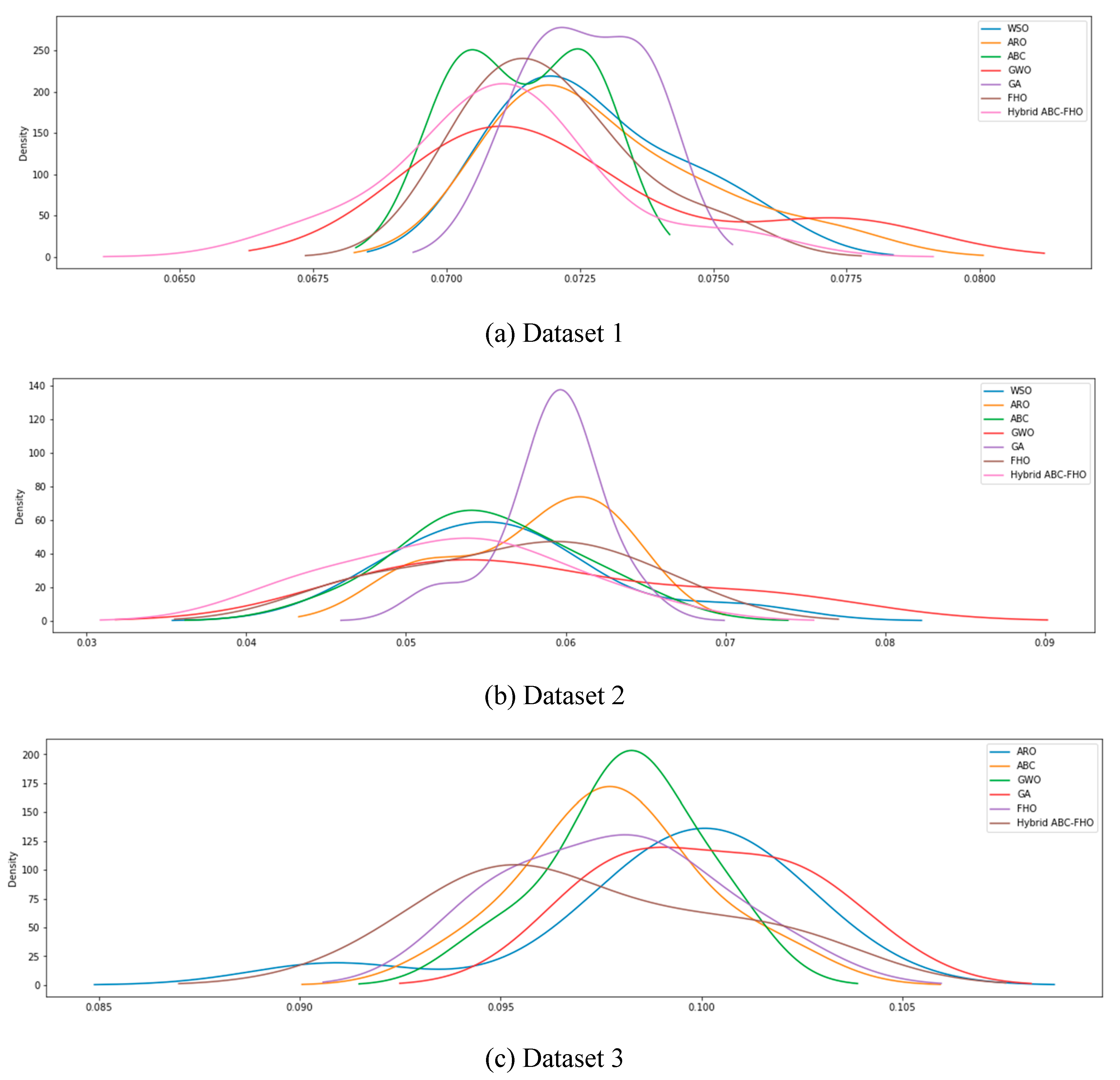
Figure 3.
5. The distribution of RMSE values across iterations.
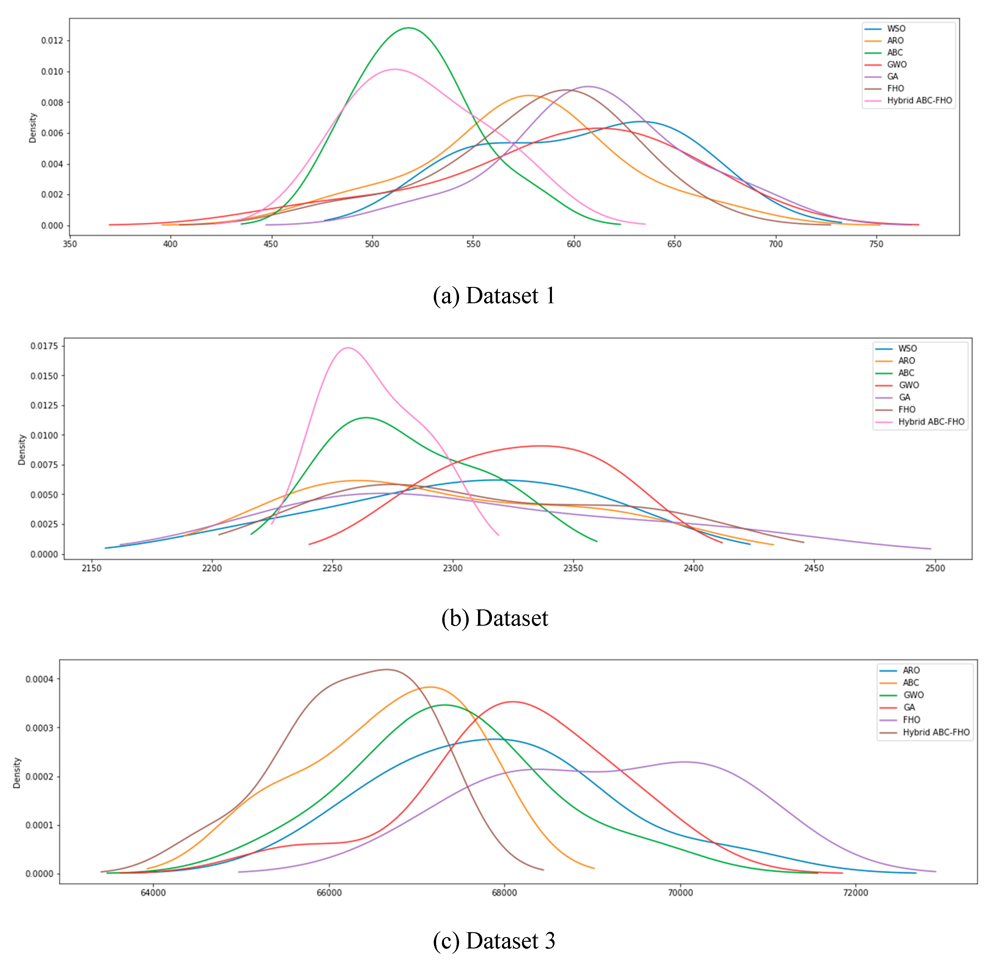
In Figure 3.4, the hybrid ABC-FHO algorithm generally exhibits narrower and more concentrated distributions across all datasets compared to other algorithms, indicating consistent accuracy with minimal performance variation. This is particularly noticeable in Dataset 1, where ABC-FHO’s density curve is tightly centered around lower MAPE values, suggesting high stability and reliability. Datasets 2 and 3 show a similar trend, with ABC-FHO maintaining one of the more stable distributions, though the overall spread is broader due to dataset complexity.
Figure 3.5 (RMSE distributions) further supports these observations. ABC-FHO displays one of the narrower distributions across all datasets, particularly in Dataset 1, where it achieves consistently low RMSE values. In Datasets 2 and 3, ABC-FHO continues to exhibit comparatively stable performance, with a reduced spread that indicates resilience in achieving accurate predictions despite variations in data characteristics.
Figure 3.6 and Figure 3.7 display the box plots of MAPE and RMSE values across multiple runs for each algorithm on Datasets 1, 2, and 3. These plots offer insights into the accuracy and stability of each algorithm. Algorithms with narrower interquartile ranges and fewer outliers exhibit more consistent performance, while those with wider distributions indicate higher variability. The box plots highlight how each algorithm’s performance fluctuates across datasets, suggesting differing levels of sensitivity to data characteristics and initial conditions. This variation in spread across MAPE and RMSE values reflects each algorithm's robustness and reliability in handling diverse forecasting scenarios.
Figure 3.
6. The box plot of MAPE values across iterations.

Figure 3.
7. The box plot of RMSE values across iterations.
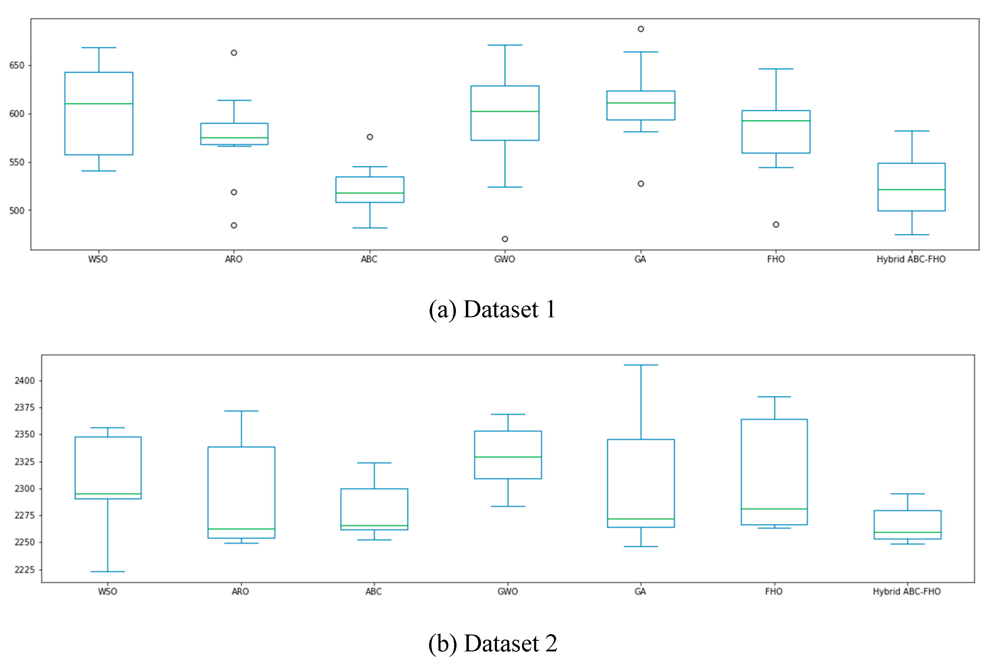
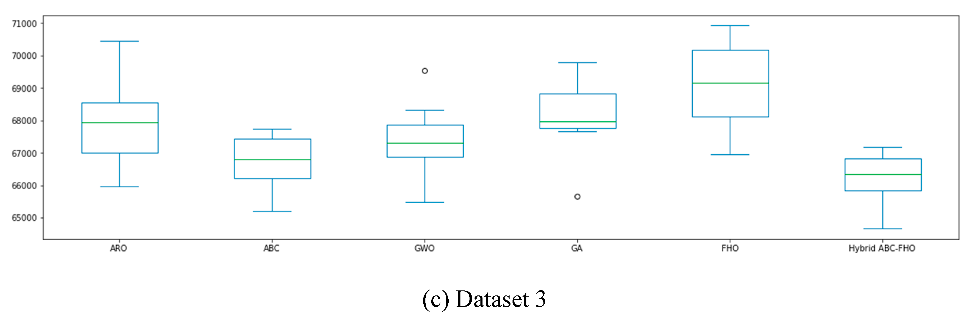
Algorithms with narrower interquartile ranges and fewer outliers demonstrate greater consistency. As shown in Figure 3.6 and Figure 3.7, the hybrid ABC-FHO algorithm, in particular, exhibits narrower spreads and fewer outliers in both MAPE and RMSE across datasets, indicating reliable and stable performance. This consistency suggests that ABC-FHO is less sensitive to data variability and initial conditions, making it a robust choice for diverse forecasting scenarios.
Table 3.8 shows the average time duration required by each algorithm to complete the forecasting tasks across the three datasets. The hybrid ABC-FHO algorithm exhibited longer computation times compared to the standalone approaches, especially for Dataset 2. However, this trade-off is justified by the superior predictive accuracy it provides. The standalone GWO algorithm was the fastest across all datasets, making it a suitable choice for scenarios where computational efficiency is critical.
Table 3.
8. The average results of time duration values of implemented algorithms.
| Dataset | GA | ARO | WSO | GWO | ABC | FHO | ABC-FHO |
|---|---|---|---|---|---|---|---|
| Dataset 1 | 15.882 | 16.677 | 15.275 | 11.694 | 21.536 | 17.110 | 23.442 |
| Dataset 2 | 45.143 | 48.612 | 45.193 | 48.897 | 60.380 | 41.552 | 68.350 |
| Dataset 3 | 18.190 | 18.068 | 17.379 | 16.512 | 20.440 | 16.256 | 22.130 |
To evaluate the statistical significance of performance differences among the algorithms, we first established a null hypothesis: The observed differences in algorithm performance are not statistically significant. To validate this, we applied the Shapiro-Wilk test to determine whether the distribution of MAPE and RMSE values for each algorithm was normal. The results of the Shapiro-Wilk test indicated non-normal distributions across all datasets, prompting the use of a non-parametric test. Given the non-normality, we conducted the Mann-Whitney U test, a robust non-parametric alternative, to assess whether the observed differences in MAPE and RMSE values between algorithms were statistically significant.
The results, presented in Table 3.11, reveal that the null hypothesis was rejected for most algorithms across datasets, indicating significant performance differences in terms of both MAPE and RMSE. These findings suggest that the differences in accuracy and error among the algorithms are not due to random variation but are statistically meaningful, reinforcing the robustness of the results.
Table 3.
11. The null (H0) hypothesis results based on the p-value.
| Dataset | Algorithms | Hypothesis (MAPE) | Hypothesis (RMSE) |
| Dataset 1 | GA | Rejected | Rejected |
| ARO | Rejected | Rejected | |
| WSO | Rejected | Rejected | |
| GWO | Rejected | Rejected | |
| ABC | Rejected | Not Rejected | |
| FHO | Rejected | Rejected | |
| Dataset 2 | GA | Rejected | Rejected |
| ARO | Rejected | Rejected | |
| WSO | Rejected | Rejected | |
| GWO | Not Rejected | Rejected | |
| ABC | Not Rejected | Rejected | |
| FHO | Rejected | Rejected | |
| Dataset 3 | GA | Rejected | Rejected |
| ARO | Rejected | Rejected | |
| WSO | Rejected | Rejected | |
| GWO | Rejected | Rejected | |
| ABC | Rejected | Rejected | |
| FHO | Rejected | Rejected |
In our experiments, conducted on three different sales datasets, the hybrid ABC-FHO algorithm consistently outperformed the other tested methods, including standalone GA, ARO, WSO, ABC, and FHO. Notably, this is the first time FHO has been applied as a standalone method in hyperparameter optimization, and it showed promising results. To ensure the reliability of our findings, we applied cross-validation and ran each model 10 times. The results were then averaged, and statistical tests were performed. These tests confirmed that the performance improvements brought by our hybrid approach were statistically significant. However, while the hybrid model excelled in prediction accuracy, it had the longest computational time among all the algorithms. In contrast, the standalone GWO was the fastest in terms of computational performance.
4. Conclusion
This study investigated the effectiveness of various metaheuristic algorithms in optimizing hyperparameters for machine learning models, with a specific focus on the hybrid ABC-FHO approach. Sales forecasting, as demonstrated, plays a crucial role in strategic decision-making within industries by enhancing operational efficiency, inventory management, and revenue optimization. In comparing multiple algorithms, including GA, ARO, WSO, GWO, ABC, and FHO, the hybrid ABC-FHO consistently emerged as a top performer across key metrics such as Mean Absolute Percentage Error (MAPE) and Root Mean Square Error (RMSE). This superior performance highlights ABC-FHO’s capability to handle complex and nonlinear sales data across diverse datasets, including Hotel Demand, Walmart, and Amazon datasets, each with unique characteristics in terms of features and data volume.
The hybrid ABC-FHO algorithm demonstrated an effective balance between exploration and exploitation, leveraging the strengths of both Artificial Bee Colony (ABC) and Fire Hawk Optimizer (FHO) algorithms. This synergy contributed to improved search efficiency, enabling ABC-FHO to navigate high-dimensional hyperparameter spaces and deliver lower error rates. By achieving lower MAPE and RMSE values, ABC-FHO proved its robustness and adaptability in handling a variety of dataset complexities, suggesting its suitability for real-world applications where data patterns and forecasting requirements vary widely.
However, this study also revealed a trade-off between accuracy and computational efficiency. While ABC-FHO delivered the best predictive accuracy, it required more computational time compared to standalone algorithms such as GWO, which demonstrated the fastest runtime across all datasets. This trade-off suggests that while ABC-FHO is suitable for tasks prioritizing accuracy, such as long-term forecasting or high-stakes decisions, it may be less ideal for real-time or time-sensitive applications where computational speed is crucial. Future work could focus on addressing this limitation by exploring parallel computing techniques or adaptive population management strategies to reduce runtime without compromising accuracy.
To further enhance the understanding of ABC-FHO’s capabilities, future research should expand the application of this hybrid algorithm to a broader range of datasets across different industries, validating its generalizability and robustness in varied sales forecasting scenarios. Additionally, the algorithm’s potential in other forecasting areas, such as customer churn prediction and demand forecasting, could be explored to evaluate its adaptability beyond sales forecasting.
In summary, the hybrid ABC-FHO algorithm presents a robust solution for hyperparameter optimization in sales forecasting, effectively balancing predictive accuracy with computational demands. This study's findings underscore the importance of hybrid algorithms in achieving reliable results for complex forecasting tasks, where data variability and model accuracy are paramount. The ABC-FHO’s performance supports its application in diverse forecasting contexts, providing a promising approach for industries aiming to enhance their predictive capabilities amidst varying data complexities and operational requirements.
Data Availability Statements
The data supporting the findings of this study are open-source and publicly available on the internet. Further details can be obtained from the corresponding author upon reasonable request.
Author Information
Department of Industrial Engineering, Yildiz Technical University, Istanbul, Türkiye Bahadir Gulsun, Muhammed Resul Aydin
Contributions
Bahadir Gulsun supervised the study, assisted in refining the study design and methodology, and performed a critical review and revision of the manuscript. Muhammed Resul Aydin conceptualized and designed the study, developed the methodology, carried out the data analysis, and prepared the manuscript draft.
Funding
No funding support.
Conflict of Interest
The authors report no conflict of interests. The authors alone are responsible for the content and writing of the paper.
References
- Abbasimehr, H., Shabani, M., & Yousefi, M. (2023). A novel hybrid machine learning model to forecast electricity prices using XGBoost, ELM, and LSTM. Energy, 263, 125546. [CrossRef]
- Abd Elaziz, M., Hosseinzadeh, M., & Elsheikh, A. H. (2023). A novel hybrid of Fire Hawk Optimizer and Artificial Rabbits Optimization for complex optimization problems. Journal of Intelligent & Fuzzy Systems, 36(2), 125-139. [CrossRef]
- Ali, A., Zain, A. M., Zainuddin, Z. M., & Ghani, J. A. (2023). A survey of swarm intelligence and evolutionary algorithms for hyperparameter tuning in machine learning models. Swarm and Evolutionary Computation, 56, 100-114.
- Al-Shourbaji, I., Hassan, M. M., & Mohamed, M. A. (2022). Hybrid ant colony optimization and reptile search algorithm for solving complex optimization problems. Expert Systems with Applications, 192, 116331.
- Ben Jabeur, H., Bouzidi, M., & Malek, J. (2024). XGBoost outperforms traditional machine learning models in retail demand forecasting. Journal of Retailing and Consumer Services, 67, 102859.
- Bindu, M. G., & Sabu, M. K. (2020). A hybrid feature selection approach using artificial bee colony and genetic algorithm. Proceedings of the IEEE International Conference on Electronics, Computing and Communication Technologies (CONECCT), 1-6.
- Braik, M., Awadallah, M. A., & Mousa, A. (2022). White Shark Optimizer: A novel meta-heuristic algorithm for global optimization problems. Applied Soft Computing, 110, 107625.
- Çetinbaş, M., Özcan, E., & Bayramoğlu, S. (2023). Hybrid White Shark Optimizer and Artificial Rabbits Optimization for photovoltaic parameter extraction. Renewable Energy, 180, 1236-1249. [CrossRef]
- Deng, Y., Zhang, J., & Liu, F. (2022). A hybrid model of XGBoost and LSTM for electricity load forecasting. Journal of Energy Storage, 46, 103568. [CrossRef]
- Dhake, P. S., Patil, A. D., & Desai, R. R. (2023). Genetic algorithm for optimizing hyperparameters in LSTM-based solar energy forecasting. Renewable Energy, 198, 75-84. [CrossRef]
- Huber, J., & Stuckenschmidt, H. (2020). Advances in seasonal and promotional sales forecasting using machine learning models. Journal of Business Research, 117, 452-461. [CrossRef]
- Jurečková, J., & Picek, J. (2007). Robust statistical methods with R. Springer.
- Katoch, S., Chauhan, S. S., & Kumar, V. (2021). A review on genetic algorithm: Past, present, and future. Multimedia Tools and Applications, 80(5), 8091-8126.
- Kaya, E., Gorkemli, B., Akay, B., & Karaboga, D. (2022). A review on the studies employing artificial bee colony algorithm to solve combinatorial optimization problems. Engineering Applications of Artificial Intelligence, 115, 105311. [CrossRef]
- Kaya, M., Karaboga, D., & Basturk, B. (2022). A comprehensive review of artificial bee colony algorithm variants and their applications. Swarm and Evolutionary Computation, 72, 101069. [CrossRef]
- MacFarland, T. W., & Yates, J. M. (2016). Introduction to nonparametric statistics for the biological sciences using R. Springer. [CrossRef]
- Makhadmeh, Z., Al Momani, M., & Mohammed, A. (2023). An enhanced Grey Wolf Optimizer for solving real-world optimization problems. Expert Systems with Applications, 213, 118834.
- Mann, H. B., & Whitney, D. R. (1947). On a test of whether one of two random variables is stochastically larger than the other. The Annals of Mathematical Statistics, 18(1), 50-60. [CrossRef]
- Massaro, M., Dumay, J., & Garlatti, A. (2021). A hybrid XGBoost-ARIMA model for improving sales forecasting accuracy in retail. Journal of Business Economics and Management, 22(4), 512-526.
- Mohakud, B. & Dash, R. (2021). Grey wolf optimization-based convolutional neural network for skin cancer detection. Journal of King Saud University - Computer and Information Sciences, 34(6), 3717-3729. [CrossRef]
- Panarese, P., Vasile, G., & Zambon, E. (2021). Sales forecasting using XGBoost: A case study in the e-commerce sector. Expert Systems with Applications, 177, 114934.
- Shapiro, S. S., & Wilk, M. B. (1965). An analysis of variance test for normality (complete samples). Biometrika, 52(3/4), 591–611. [CrossRef]
- Tran, Q. A., Nguyen, D. K., & Le, T. H. (2020). Enhancing long-term meteorological predictions with genetic algorithms and LSTM networks. IEEE Access, 8, 29832-29843.
- Zhang, X., Wu, Y., & Li, Z. (2021). A comparison of XGBoost and ARIMA in demand forecasting of e-commerce platforms. Electronic Commerce Research and Applications, 45, 101030.
- Zulfiqar, U., Rehman, M. U., & Khan, A. (2022). Adaptive differential evolution and support vector machines for load forecasting. Electric Power Systems Research, 208, 107976. [CrossRef]
Table 3.
4. The selected lower bounds and upper bounds search area in the case study.
| Hyperparameters | Lower Bound | Upper Bound |
|---|---|---|
| colsample_bytree | 0.5 | 1 |
| n_estimators | 50 | 1000 |
| max_depth | 2 | 15 |
| learning_rate | 0.01 | 5 |
| min_child_weight | 0.001 | 10 |
| reg_alpha | 0 | 1 |
| reg_lambda | 0 | 1 |
| subsample | 0.5 | 1 |
| num_leaves | 10 | 900 |
Disclaimer/Publisher’s Note: The statements, opinions and data contained in all publications are solely those of the individual author(s) and contributor(s) and not of MDPI and/or the editor(s). MDPI and/or the editor(s) disclaim responsibility for any injury to people or property resulting from any ideas, methods, instructions or products referred to in the content. |
© 2024 by the authors. Licensee MDPI, Basel, Switzerland. This article is an open access article distributed under the terms and conditions of the Creative Commons Attribution (CC BY) license (https://creativecommons.org/licenses/by/4.0/).
Copyright: This open access article is published under a Creative Commons CC BY 4.0 license, which permit the free download, distribution, and reuse, provided that the author and preprint are cited in any reuse.


