
Submitted:
07 November 2024
Posted:
11 November 2024
You are already at the latest version
Abstract
In this paper, we have developed an explicit symmetric six-step method. This new method is phase-fitted and incorporates a free coefficient as a parameter. Using a wide range of values for this parameter, we computationally define the periodicity interval. Numerical outcomes guided us toward identifying optimal values for the parameter, establishing the new method’s high efficiency. The efficiency of the new method is demonstrated through its application to oscillatory problems, comparing it with well-known phase-fitted methods.
Keywords:
Linear multistep methods
; Ordinary differential equations
; Initial value problems
; Phase-lag
1. Introduction
This paper focuses on the numerical solution of the initial value problem (IVP) characterized by the following form
whose solutions display a notable oscillatory nature. This kind of problem is commonly encountered across a wide spectrum of scientific disciplines, such as quantum mechanical scattering problems, celestial mechanics, and elsewhere.
Several authors have derived numerical methods of a single step, such as Runge-Kutta or Runge-Kutta-Nyström, which are based on properties such as phase-lag or trigonometric / exponential fitting (see [1,2,3,4,5,6]), while others use these properties for the development of multistep methods (see [7,8,9,10,11,12,13,14,15,16,17,18,19,20]). All of these methods incorporate frequency-dependent coefficients and demonstrate high efficiency in numerical solution of second-order IVPs with oscillating solutions.
In this research work, a new explicit parametric symmetric linear six-step method is produced. The new method is of sixth algebraic order with zero phase-lag and is used for the numerical solution of oscillatory problems. The approach of this study is based on the procedure of Anastassi and Simos [12] for the derivation of a linear four-step method, and should be considered as a technique which gives the opportunity to choose the appropriate value for the free parameter in order to numerically solve an IVP, depending on whether it needs a fast low accurate solution or a solution of high accuracy.
In particular, in Section 2, the basic theory of linear multistep methods is provided. In Section 3, the development of the new parametric method is presented, as well as the local truncation error and periodicity analysis for the new method. Furthermore, in Section 4, the results of the application to three well-known problems are demonstrated. Finally, the conclusions of this research article are presented in Section 5.
2. Theory of Linear Multistep Methods
The linear k-step method for the numerical integration of the initial value problem (1) is of the form
The general method (2) it is known that is associated with the linear difference operator which is given from the expression
where
Definition 1.
At this point, we consider the scalar test equation
By applying a 2k-step symmetric method to equation (4), the difference equation below is produced
where are polynomials in v of the form and .
The characteristic equation which is associated with (5) is
The following definitions are derived from Lambert and Watson [21].
Definition 2.
A symmetric 2k-step method with characteristic equation of the form (6) has interval of periodicity , if the characteristic roots should satisfy the following conditions:
and ,
where and is a real function of s.
Definition 3.
For any method corresponding to the characteristic equation (6), the phase-lag is defined as the term .
If the quantity as , the order of phase-lag is q, where the characteristic roots are of the form and satisfy the conditions of Definition (2)
Theorem 1.
The symmetric 2k-step method with characteristic equation given by (6) has phase-lag q and phase-lag constant c given by
3. Development of the New Symmetric Method
This section outlines the derivation approach for an explicit symmetric linear six-step method featuring frequency-dependent coefficients.
With this objective in mind, we examine the following scheme
The linear method we are about to formulate is of sixth algebraic order and incorporates a variable coefficient as a parameter. This coefficient will be utilized to explore both accuracy and the interval of periodicity. If we apply the six-step method (8) on the scalar equation (4), we generate the polynomials , with , where represents the primary frequency of the problem and h denotes the integration step size. Subsequently, using Theorem (1), we derive the expression for the method’s phase-lag (PL).
To attain both zero phase-lag and the highest achievable algebraic order p for method (8), the following conditions must be satisfied
Upon solving the aforementioned system, we obtain the expressions for the method’s coefficients.
As , instead of using the above expressions, we use the Taylor series expansions.
3.1. Local Truncation Error and Periodicity Analysis
Using the expressions (13) into the method (8), we derive the principal error for the test equation (4). This error arises from the Taylor series expansion of the difference between both sides of Equation (8) and its expression is as follows.
At this point, we computationally determine the interval of periodicity. Following the application of method (8) using the coefficients outlined in (12) to address the test problem (4), we calculate the characteristic equation for the new parametric method as defined in Equation (6). The characteristic equation obtained is expressed as follows.
where:
We perform computational analysis on the characteristic equation (15) over a broad spectrum of coefficient values, . In this process, we ascertain the periodicity interval by assessing the conditions stipulated in Definition 2 for the set , where and . The results of this investigation are illustrated in Figure 1.
It is important to emphasize that the method exhibits a non-zero periodicity interval exclusively when falls within the range of . Furthermore, the method displays convergence within this identical interval due to its inherent consistency. As depicted in Figure 1, the reduction in the value of , corresponds to an expansion of the periodicity interval. In addition, a similar behavior is observed in the case of the local truncation error, evident from Equation (14), and notably from the expression . This expression reaches its maximum value as approaches and its minimum value as tends towards . Therefore, the objective is to identify the optimal value of that simultaneously minimizes the error and ensures the stability of the method.
4. Numerical Results
4.1. The Problems
The recently introduced method, described above, was applied to three widely recognized oscillatory problems.
- The Schrödinger equation - Resonance problem
- The "almost" periodic orbit problem by Stiefel and Bettis
- The Duffing equation
The description of these problems is given below.
4.1.1. Schrödinger Equation - Resonance Problem
The one-dimensional or radial Schrödinger equation has the form
where
,
E is the energy,
is the centrifugal potential,
the electric potential
The function is the effective potential, where and so . Furthermore, there is the boundary condition and a second boundary condition, which is determined by physical considerations for large values of x.
For our numerical illustration, we will consider the integration domain as , applying the Woods-Saxon potential
For positive energies , the potential dies away faster than the centrifugal potential , so for large values of x, Schrödinger equation effectively reduces to
Equation has two linearly independent solutions. These are and , where and represent the spherical Bessel and Neumann functions, respectively. As , the solution to equation takes the following asymptotic form.
where is the scattering phase shift, which may be approximated by the following expression.
where and both exist in the asymptotic region.
In the case of positive energies () and for , we approximate based on (20) and then compare its value to the exact value . For this eigenvalue problem the boundary conditions are and for large x.
We use the eigenenergy and for the frequency we use the suggestion of Ixaru and Rizea [22]
4.1.2. Orbit problem by Stiefel and Bettis
Stiefel and Bettis (1969) [23] studied the "almost" periodic orbit problem, which is given below.
where .
The analytical solution of the problem (21) is
Equivalently, the problem (21) can be described from the system
The analytical solution of the system (22) is
The estimated frequency for this problem is .
4.1.3. Duffing equation
The Duffing equation can be described by
where
The analytical solution of (23) is
where
,
,
,
and
The estimated frequency for this problem is .
4.2. The Compared Methods
To evaluate the efficiency of the new method, we compare it with five well-known sixth algebraic order phase-fitted explicit methods with variable coefficients. The methods used in the comparison are
- Method A: The new phase-fitted parametric method which was derived in Section 3 (for a wide range of parameter ).
- Method B: The 4-step phase-fitted method, developed by Simos [9].
- Method C: The Numerov-type hybrid method, developed by Konguetsof [14].
- Method D: The Runge-Kutta type hybrid method, developed by Alolyan and Simos [11].
- Method E: The zero-dissipative hybrid method, developed by Ahmad et. al [10].
- Method F: The high order method of the Runge-Kutta-Nyström pair, developed by Anastassi and Kosti [1].
4.3. Effectiveness and Optimal Values for the New Parametric Method
In Figure 2 - Figure 4, we visualize the evaluation of the novel parametric approach, which is represented as , relative to the coefficient . The error in this context is determined differently for distinct scenarios: in the case of known accurate solutions such as the Stiefel-Bettis problem and the Duffing equation, the error corresponds to the maximum absolute error value of the integration interval. In the case of Schrödinger equation, the error is defined as .
Each of these figures illustrates the accuracy of the new method, represented by small dots (appearing as solid lines) across all values of the parameter and for various integration step sizes h. As expected, smaller integration steps result in higher accuracy. The variety of colors in the graphs corresponds to different integration step lengths, as indicated in the figures’ legends. The dashed line, shown in a specific color, signifies the highest level of accuracy achieved by alternative methods in the comparative analysis (see Section 4.2) while requiring the same computational effort — measured as of the number of function evaluations — as the new parametric method.
For instance, in the case of the Stiefel and Bettis problem (Figure 4), when the new method is employed with a step size of , its initial accuracy is relatively low () for values of . However, it progressively improves, surpassing an accuracy level of 8 as . Among the other methods subjected to the same number of function evaluations required by the new method (for ), the most efficient demonstrates an accuracy of approximately , denoted by the same color dashed horizontal line (as accuracy for the other methods does not depend on the coefficient ). The intersection points reveal that the new parametric method consistently outperforms the other methods under consideration for all values of exceeding approximately . Points where the graph lacks small dots indicate that the parametric method exhibits instability. This typically occurs when employing large step-size values (h) and for high values of the coefficient ().
Furthermore, in terms of effectiveness, there exists a substantial range of values for the coefficient , where the new method consistently delivers the highest level of accuracy. These specific intervals commence at the point of intersection between the small dots and the dashed line. For the Schrödinger equation, this interval begins at approximately , for the Duffing equation at , and for the Stiefel-Bettis problem it starts at .
Regarding the upper limit of this interval, it varies depending on whether our priority is to obtain a highly accurate solution or a faster, albeit less accurate one. In pursuit of enhanced accuracy, our objective is to choose a value for that closely approaches the upper limit of this interval. When our aim is to achieve a quicker solution with reduced accuracy, for example, an accuracy level of 1 or 2, it becomes necessary to adjust the upper limit of the interval within which operates in order to maintain method’s stability. Specifically, these adjusted upper limits are as follows: for the Schrödinger equation and for the rest of the problems.
The new method’s accuracy exhibits occasional spikes across different combinations of h and values. These spikes are a result of resonances triggered by the presence of spurious roots within the characteristic equation of the method. It’s essential to recognize that these resonances vary for different values of , and this phenomenon is inherent in all linear multistep methods comprising more than two steps. Quinlan’s extensive investigation of this behavior, with further details available in [24], sheds light on the matter. Fortunately, when considering the recommended optimal values outlined below, the new method consistently outperforms the compared methods.
Considering the examination presented in the preceding paragraphs, the recommended values for the coefficient are presented in Table 1.
4.4. Comparison of the New Parametric Method with Other Phase-Fitted Methods Based on Optimal Values and Upper Limits for
At this point, we demonstrate the accuracy of the new method against the phase-fitted methods described in Section 4.2 by choosing a value for the coefficient based on the upper limits discussed in Section 4.3. We choose to measure the efficiency of the method by computing the accuracy in the decimal digits, which is (maximum error through the integration intervals) versus the computational effort measured by the (number of function evaluations required).
Following the analysis preceded in Section 4.3, we choose for the parameter the value , which is the upper limit of the interval for the Schrödinger equation. In Figure 5 - Figure 7, we display the results. According to the results, the proposed method demonstrates superior effectiveness in all three problems, achieving higher accuracy than the other methods in the comparison.
5. Conclusions
This study introduces a six-step parametric phase-fitting method with frequency-dependent coefficients for the numerical solution of oscillatory problems. We evaluated the efficiency of our new method across a wide spectrum of parameter’s value and conducted a comparative assessment against established methods in the existing literature. The numerical results guided us toward identifying optimal values for the parameter, establishing the high efficiency of the new method.
Funding
This research received no external funding.
Institutional Review Board Statement
Not applicable.
Informed Consent Statement
Not applicable.
Data Availability Statement
Not applicable.
Acknowledgments
The publication fees of this manuscript have been financed by the Research Council of the University of Patras.
Conflicts of Interest
The authors declare no conflicts of interest.
References
- Anastassi, Z.A.; Kosti, A. A 6(4) optimized embedded Runge–Kutta–Nyström pair for the numerical solution of periodic problems. Journal of Computational and Applied Mathematics 2015, 275, 311–320. [Google Scholar] [CrossRef]
- Monovasilis, T.; Kalogiratou, Z. High order two-derivative runge-kutta methods with optimized dispersion and dissipation error. Mathematics 2021, 9, 232. [Google Scholar] [CrossRef]
- Papadopoulos, D.F.; Simos, T.E. A new methodology for the construction of optimized Runge–Kutta–Nyström methods. International Journal of Modern Physics C 2011, 22, 623–634. [Google Scholar] [CrossRef]
- Papadopoulos, D.F.; Anastassi, Z.A.; Simos, T.E. A phase-fitted Runge–Kutta–Nyström method for the numerical solution of initial value problems with oscillating solutions. Computer Physics Communications 2009, 180, 1839–1846. [Google Scholar] [CrossRef]
- Papadopoulos, D.F.; Anastassi, Z.A.; Simos, T.E. The Use of Phase-Lag and Amplification Error Derivatives in the Numerical Integration of ODEs with Oscillating Solutions. International Conference on Numerical Analysis and Applied Mathematics. AIP Conference Proceedings, 2009, pp. 547–549.
- Tsitouras, C.; Famelis, I.T.; Simos, T.E. Phase-fitted Runge–Kutta pairs of orders 8(7). Journal of Computational and Applied Mathematics 2017, 321, 226–231. [Google Scholar] [CrossRef]
- Simos, T.E. Dissipative trigonometrically fitted methods for the numerical solution of orbital problems. New Astronomy 2003, 9, 59–68. [Google Scholar] [CrossRef]
- Simos, T.E. An explicit four-step method with vanished phase-lag and its first and second derivatives. Journal of Mathematical Chemistry 2014, 52, 833–855. [Google Scholar] [CrossRef]
- Simos, T.E. An explicit four-step method for the numerical integration of second-order initial-value problems. Journal of Computational and Applied Mathematics 1994, 55, 125–133. [Google Scholar] [CrossRef]
- Ahmad, S.; Ismail, F.; Senu, N.; Suleiman, M. Zero-dissipative phase-fitted hybrid methods for solving oscillatory second order ordinary differential equations. Applied Mathematics and Computation 2013, 219, 10096–10104. [Google Scholar] [CrossRef]
- Alolyan, I.; Simos, T.E. A new high order two-step method with vanished phase-lag and its derivatives for the numerical integration of the Schrödinger equation. Journal of Mathematical Chemistry 2012, 50, 2351–2373. [Google Scholar] [CrossRef]
- Anastassi, Z.A.; Simos, T.E. A parametric symmetric linear four-step method for the efficient integration of the Schrödinger equation and related oscillatory problems. Journal of Computational and Applied Mathematics 2012, 236, 3880–3889. [Google Scholar] [CrossRef]
- Anastassi, Z.A.; Simos, T.E. New Trigonometrically Fitted Six-Step Symmetric Methods for the Efficient Solution of the Schrödinger Equation. MATCH 2008, 60, 733–752. [Google Scholar]
- Konguetsof, A. Two-step high order hybrid explicit method for the numerical solution of the Schrödinger equation. Journal of Mathematical Chemistry 2010, 48, 224–252. [Google Scholar] [CrossRef]
- Medvedeva, M.A.; Simos, T.E. A multistep method with optimal phase and stability properties for problems in quantum chemistry. Journal of Mathematical Chemistry 2022, 60, 937–968. [Google Scholar] [CrossRef]
- Panopoulos, G.; Anastassi, Z.A.; Simos, T.E. Two optimized symmetric eight-step implicit methods for initial-value problems with oscillating solutionsn. Journal of Mathematical Chemistry 2009, 46, 604–620. [Google Scholar] [CrossRef]
- Psihoyios, G.; Simos, T.E. A New Trigonometrically-Fitted Sixth Algebraic Order P-C Algorithm for the Numerical Solution of Radial Schrödinger Equation. Mathematical and Computer Modelling 2005, 42, 887–902. [Google Scholar] [CrossRef]
- Raptis, A.; Allison, A. Exponential-fitting methods for the numerical solution of the schrödinger equation. Computer Physics Communications 1978, 14, 1–5. [Google Scholar] [CrossRef]
- Wang, Z. P-stable linear symmetric multistep methods for periodic initial-value problems. Computer Physics Communications 2005, 171, 162–175. [Google Scholar] [CrossRef]
- Coleman, J.; Ixaru, L. P-stability and exponential-fitting methods for y” = f (x, y). IMA Journal of Applied Mathematics 1996, 16, 179–199. [Google Scholar] [CrossRef]
- Lambert, J.D.; Watson, I.A. Symmetric multistep methods for periodic initial values problems. IMA Journal of Applied Mathematics 1976, 18, 189–202. [Google Scholar] [CrossRef]
- Ixaru, L.; Rizea, M. A numerov-like scheme for the numerical-solution of the Schrödinger-equation in the deep continuum spectrum of energiess. Computer Physics Communications 1980, 19, 23–27. [Google Scholar] [CrossRef]
- Stiefel, E.; Bettis, D.G. Stabilization of Cowell’s Method. Numer. Math. 1969, 13, 154–175. [Google Scholar] [CrossRef]
- Quinlan, G. Resonances and instabilities in symmetric multistep methods. arXiv:astro-ph/9901136v1, 1999. [Google Scholar]
Figure 1.
Method’s periodicity interval with respect to the coefficient
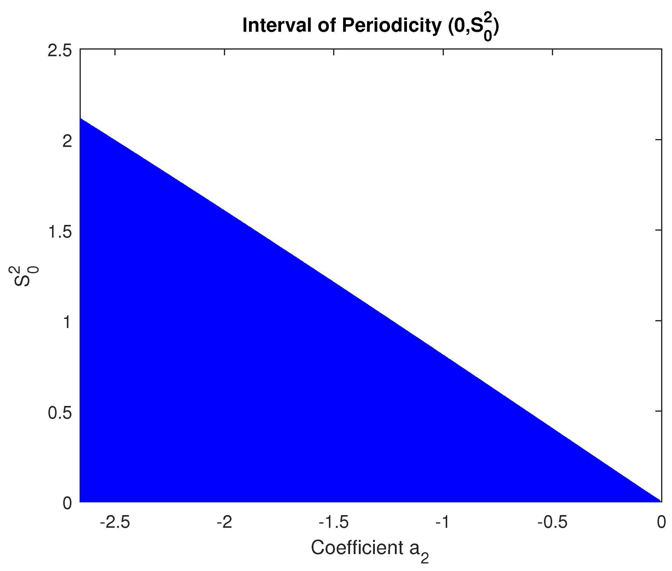
Figure 2.
Efficiency of the new method for all values of - Schrödinger equation
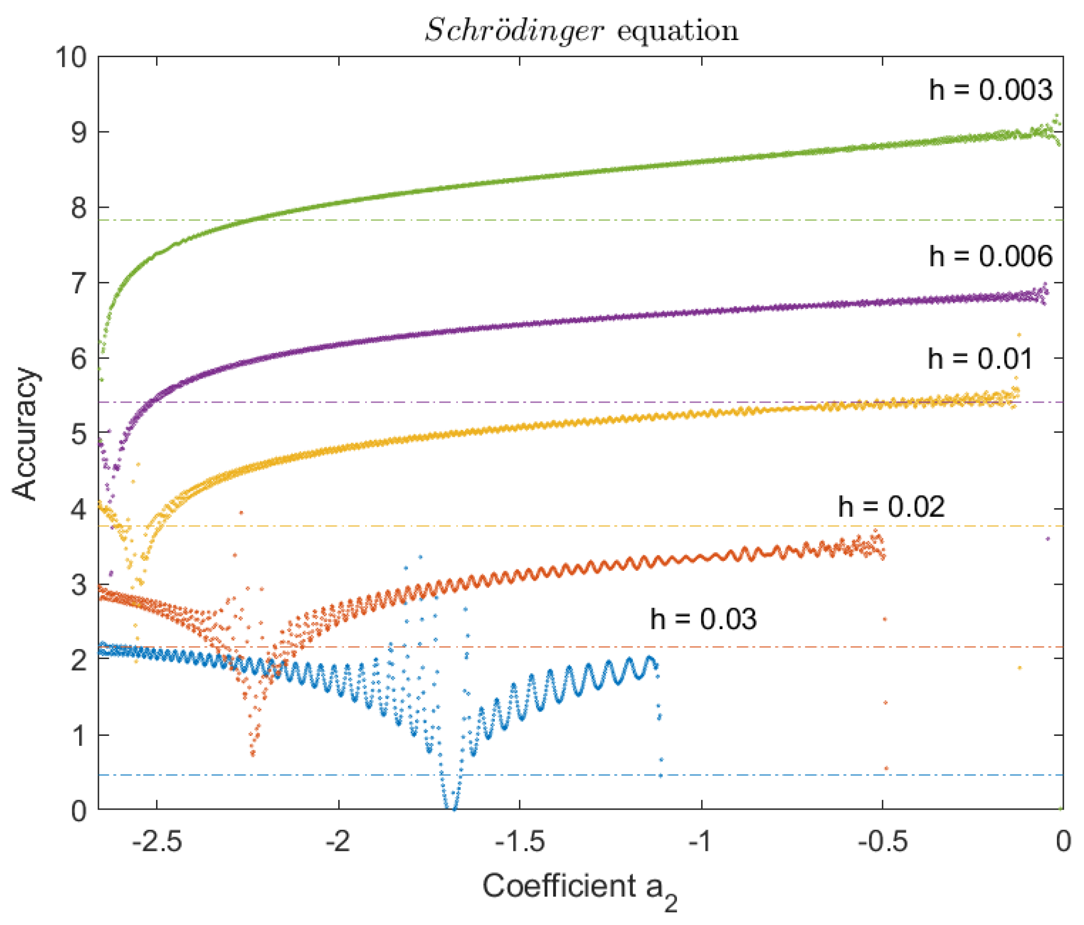
Figure 3.
Efficiency of the new method for all values of - Duffing equation
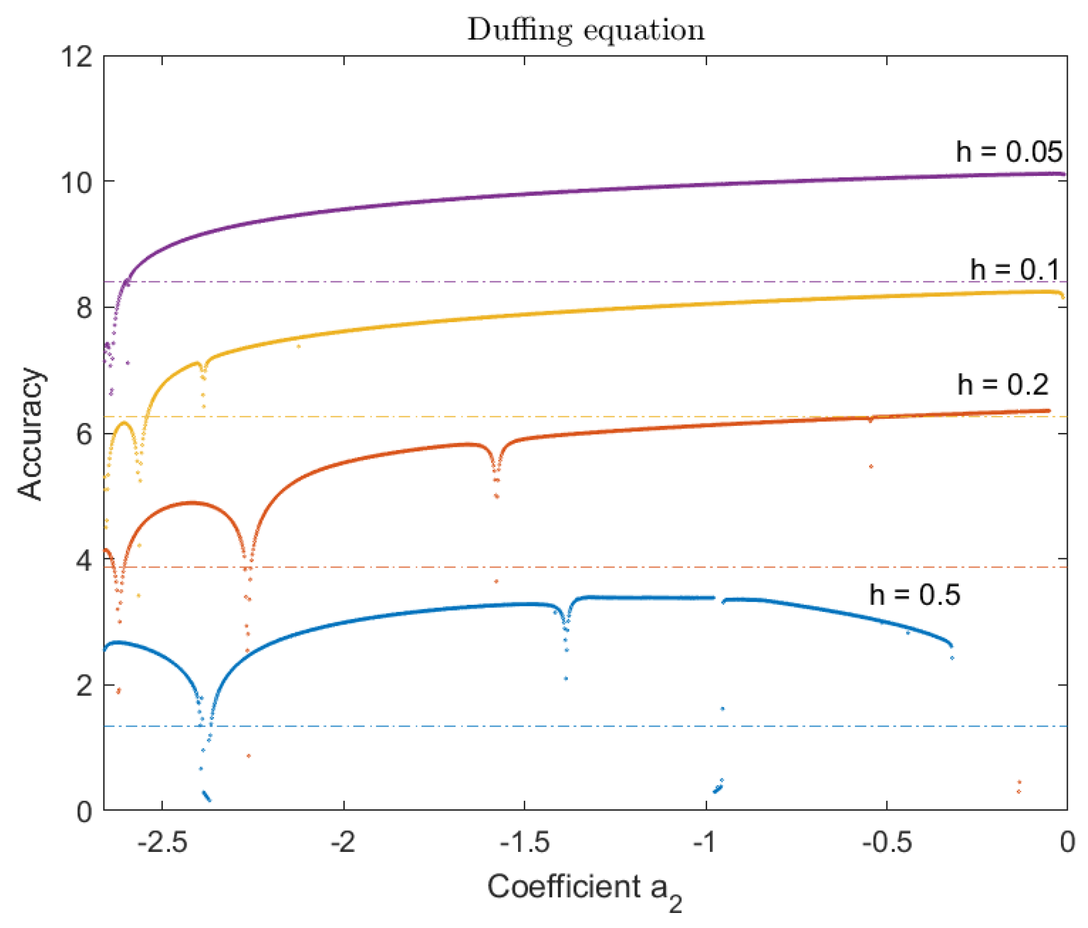
Figure 4.
Efficiency of the new method for all values of - Stiefel-Bettis problem
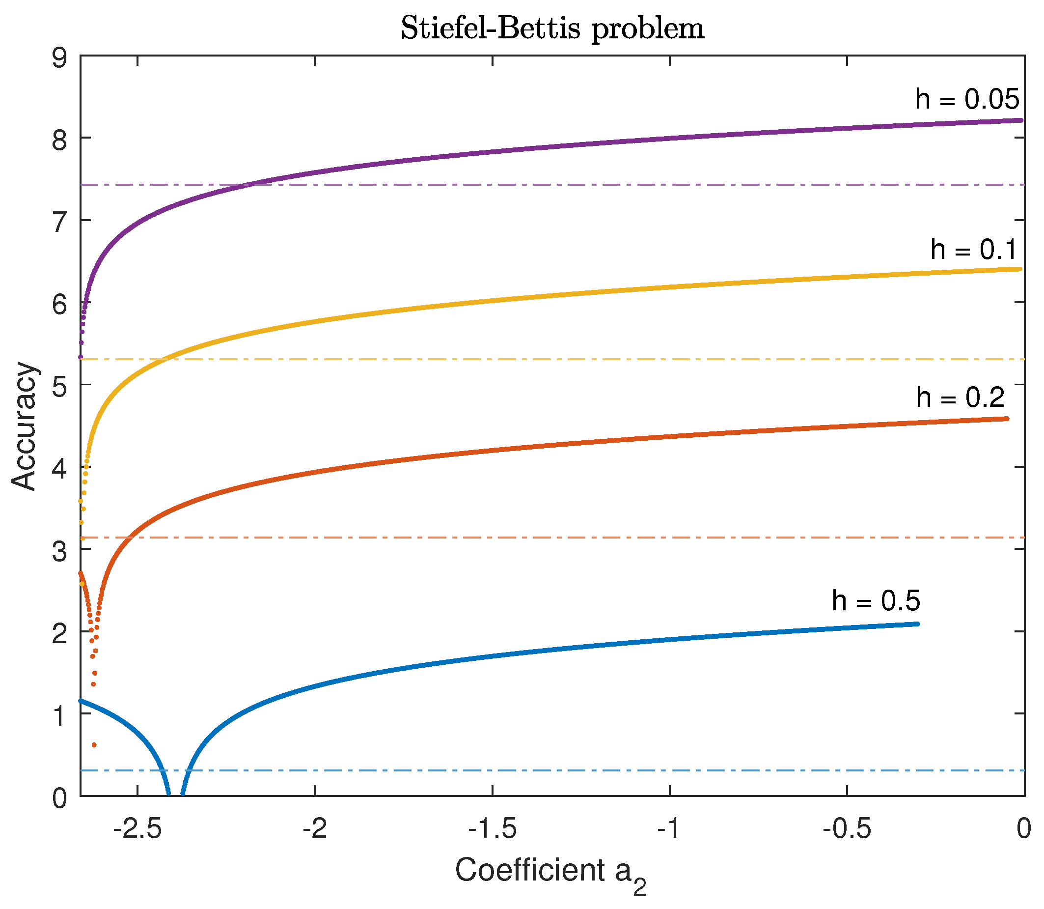
Figure 5.
Comparison for the Schrödinger equation
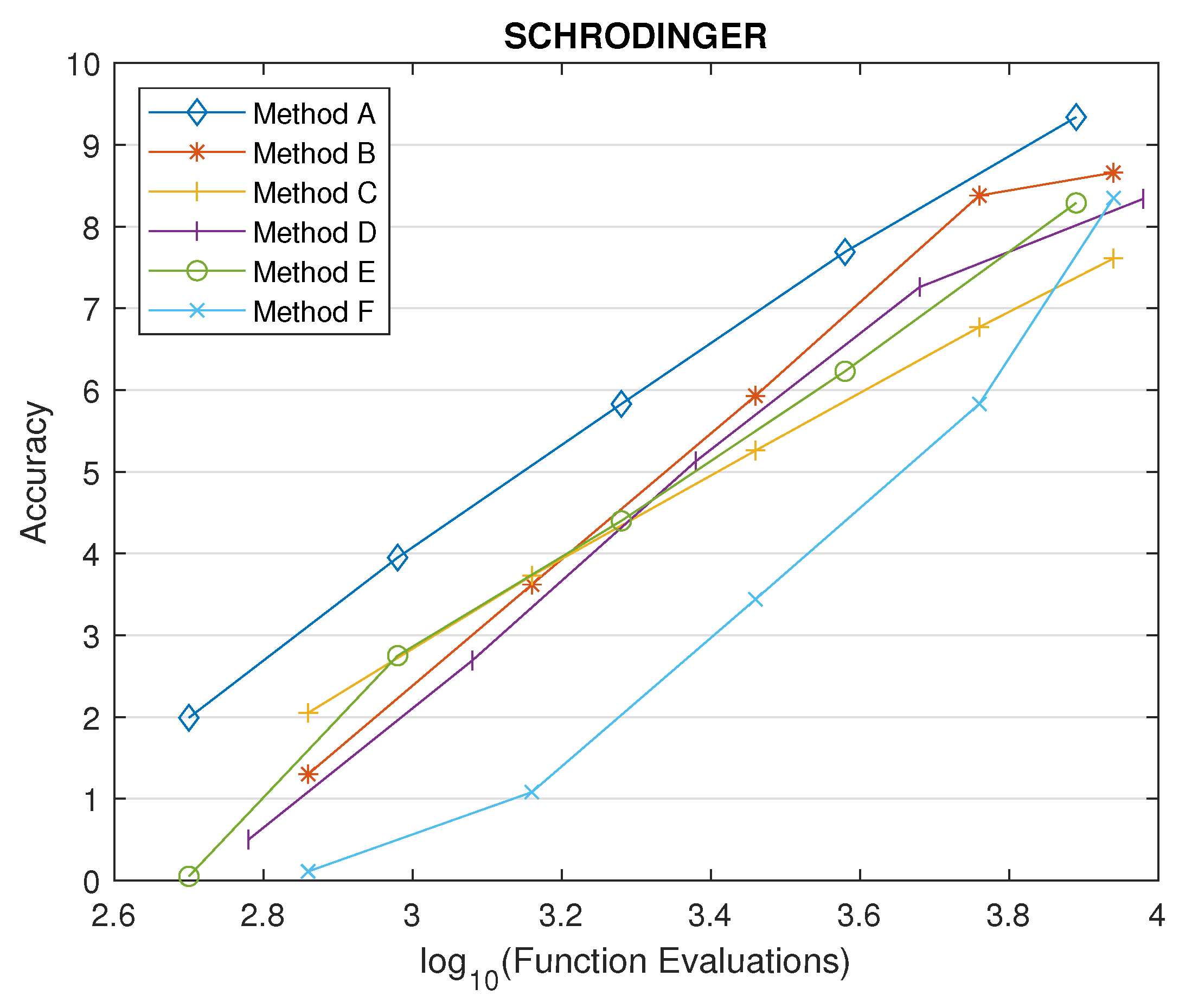
Figure 6.
Comparison for the Duffing equation
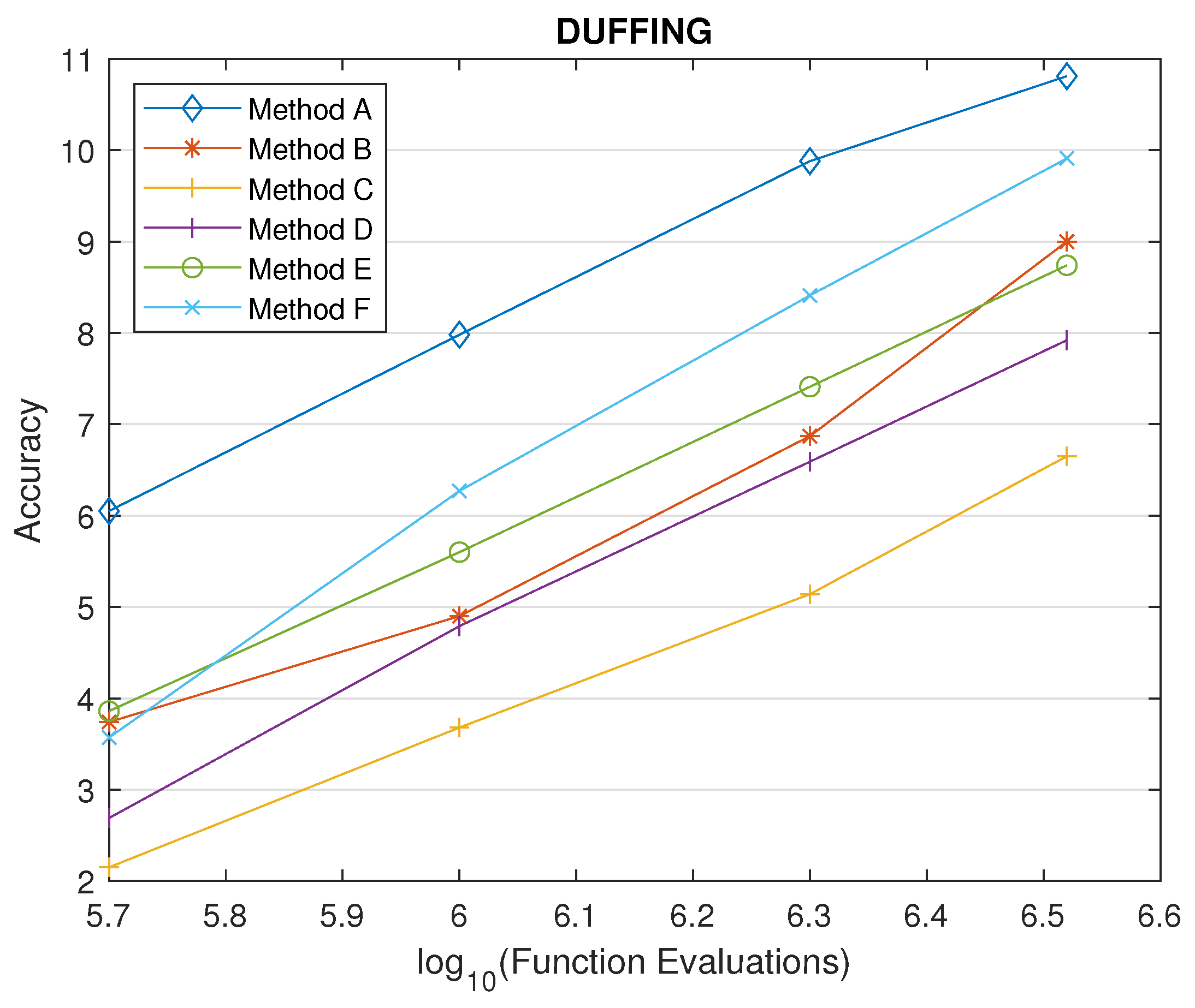
Figure 7.
Comparison for the Stiefel-Bettis problem
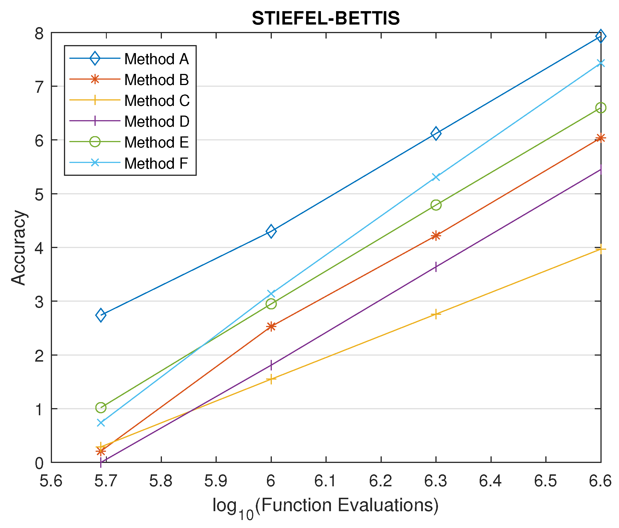

Table 1.
Optimal values of the parameter .
| Value of | Accuracy |
|---|---|
| for high accuracy () | |
| for fast solution with low accuracy () | |
| for medium accuracy |
Disclaimer/Publisher’s Note: The statements, opinions and data contained in all publications are solely those of the individual author(s) and contributor(s) and not of MDPI and/or the editor(s). MDPI and/or the editor(s) disclaim responsibility for any injury to people or property resulting from any ideas, methods, instructions or products referred to in the content. |
© 2024 by the author. Licensee MDPI, Basel, Switzerland. This article is an open access article distributed under the terms and conditions of the Creative Commons Attribution (CC BY) license (https://creativecommons.org/licenses/by/4.0/).
Copyright: This open access article is published under a Creative Commons CC BY 4.0 license, which permit the free download, distribution, and reuse, provided that the author and preprint are cited in any reuse.


