
Submitted:
06 November 2024
Posted:
11 November 2024
You are already at the latest version
Abstract
A flood is defined as a relatively high flow rate or water level in a river or body of water, characterized by an elevation above the norm, leading to the inundation of low-lying areas or bodies of water that are not normally submerged. Almost every year, floods of significant magnitude impact the Nokoue lake basin, endangering nearby populations as they greatly affect the economy and infrastructure development. The unresolved issue of flooding in Nokoue lake necessitates a thorough study and analysis of specific flow models, particularly those concerning the frequency, probability, and scale of flooding. In this context, the present article on threshold determination and flood frequency analysis is highly valuable in mitigating the chronic flooding problem of Nokoue lake. Flood frequency analysis involves interpreting the historical flood data and predicting future probabilities. Annual data on the maximum water level of Nokoue lake over 27 years, from 1997 to 2022, was used for this purpose. The peak water level indices of Nokoue lake and classification were used to characterize flood thresholds. The Gumbel extreme value distribution method, the generalized extreme value distribution method, and the generalized Pareto method were used to test the probability of flood occurrence. The analysis results indicate that flood hazard thresholds are defined as follows: from negative infinity up to below 3.94 m for limited risk, from 3.94 m up to 4.04 m for moderate risk, from above 4.04 m to 4.14 m for significant risk, and from above 4.14 m to 4.95 m for critical risk. Among the flood frequency analysis methods, the Gumbel extreme value distribution is considered more effective and suitable for estimating flood occurrence probabilities and for designing flood control measures for Nokoue lake with a root mean square error (RMSE) of 0.0724, compared to 0.0754 and 0.0761 for the GEV and GPA distributions, respectively. The position and scale parameters (φ; α) of the Gumbel distribution were estimated to be 3.802 and 0.249, respectively. This allows for the calculation of the probability of an extreme water level occurring within a return period in a single day. Thus, the extreme water levels (flood quantiles) associated with return periods of 10, 50, and 100 years, as determined by the Gumbel distribution, are 4.36m, 4.77m, and 4.95m, respectively. Exceptional and very exceptional hydrological events have return periods of 100 and 150 years, corresponding to peak flow levels ranging from 4,95m and 5,05m respectively. These values are of crucial importance for the design of flood prevention structures (infrastructure) intended to mitigate flood risk.
Keywords:
flood hazard thresholds
; flood risk
; frequency analysis
; statistical distributions
; probability
; water level peaks
1. Introduction
Floods are currently the most frequent and damaging natural risk in West Africa. [1], [2,3,4]. They have harmful effects on the activities and populations living along the banks and involve significant security challenges for the most exposed areas. They are natural phenomena that are integral to the natural regime of water bodies (lakes) and watercourses (rivers), and protection against them requires prevention and forecasting [5,6,7]. Unlike the management approaches of the 1960s, current policies tend to better account for the significant role of floods and the means of managing the flood risk of a water body or a watercourse. Flood risk is particularly complex to understand due to its random nature associated with climate change, especially in highly developed and urbanized areas such as urban and peri-urban zones [8,9,10]. This issue is also present in the Nokoue lake watershed. The basin is indeed subject to high rainfall intensities that can be potentially devastating due to the rapid urban growth along its banks. Scientific literature has shown that, regardless of the nature of the floods, hydrological studies are often overlooked, and flood prevention structures are poorly designed due to the use of outdated empirical formulas [11,12,13]. Therefore, to reduce anxiety about the threat of flooding from Nokoue lake in Benin, the estimation of extreme water level is used in the context of public policy implementation for risk prevention or coastal management, particularly through the characterization of flood hazards. The purpose of these estimations is to provide a high level of safety in flood risk prevention. In this study, we apply probabilistic models to estimate extreme water level up to a 100-year return period for Nokoue lake. The estimates are made using an extreme value statistical analysis method. The choice of a 100-year return period is driven by political rather than scientific reasons. However, the estimation of extreme surcharges (quantiles) for return periods close to 100 years is useful for analyzing rare extreme events. The results of this study could provide valuable insights for evaluating the extreme scenarios referenced by public policies in flood risk prevention for Nokoue lake.
2. Materials and Methods
2.1. Study areas
Nokoue lake is located in southern Benin between 6°38' and 6°50' North latitude, and 2°35' and 2°55' West longitude. It extends between 150 and 170 km², respectively, during the low water period and the high-water period (Figure 1).
2.2. Statistic Description of Water Level Peaks Values
This study focuses on the statistical analysis of annual water level peaks of Nokoue lake, sourced from the Institute of Hydrology and Oceanology Research of Benin (IRHOB). An annual water level peak is defined as the maximum observed value within a year. These values were extracted from a daily data collecting covering the period from 1997 to 2022.
2.3. Standaedized Water Level Peaks Indices Calculation and Categorization of Flood Hazard
The identification of flood hazard thresholds is based on three steps: the calculation of standardized water level index, the representation of standardized index based on annual water level peaks, and the projection of normalized water level index on to the x-axis showing the annual water level peaks. The categorization of flood risk alert thresholds for Nokoue lake is based on the standardized water leval index inspired by McKee's study. By normalizing the annual water level peaks series of nokoue lake, these thresholds were determined [15,16,17]. The formula for the water level index is as follows.
Where is the water level index, is the observed annual maximum value, the mean of the annual peak water level values, the standard deviation of the annual water level peaks values. The different risk categories such as: limited, moderate, significant, and critical are shown in Table 1.
2.4. Implementation of Frequency Models
Extreme water levels are estimated using a method of statistical fitting and extrapolation of extremes. Only the main points of the method are outlined here. For more information, please refer to [14]. The calculations were performed using the R environment because it is well known nowadays well. The methodology for establishing frequency fitting curves consists of three main steps: (i) statistical tests (stationarity, independence, and homogeneity), (ii) Selection and calculation of empirical probabilities of the extracted annual water level peak values and (iii) fitting to estimate parameters of the distribtuion and quantiles corresponding to several specified return periods associated with exceedance frequencies.
- Hypothesis testing.
The Mann-Kendall, Wald-Wolfowitz, and Wilcoxon tests were used respectively for stationarity, independence, and homogeneity. The p-value represents the risk of error if we consider that the null hypothesis (the hypothesis that the sample is stationary, homogeneous, and independent) is not true. The maximum acceptable value for the risk of error is set at 5%. If the p-value is less than 5%, there is less than a one in five chance of being wrong in considering that the series of annual water level peaks is not independent, stationary, and homogeneous [19].
- ✓
- Stationarity test
A series of random variables is said to be stationary if its statistical characteristics (mean, variance, or moments) remain invariant over time [19]. The Mann-Kendall test was used to verify stationarity, allowing us to test the following hypotheses:
- -
- H0: The statistical characteristics of the random variables are constant over time.
- -
- H1: The statistical characteristics of the random variables are not constant over time.
Given random variables arranged in chronological order, the test statistic is expressed as follows:
Under hypothesis , the statistic asymptotically follows a normal distribution with a mean of zero and a variance . The closer the test statistic is to zero, the more the observations are considered to be stationary.
- ✓
- Independence test
A data series is said to be independent if one data point is not influenced by the preceding data point [20]. For the implementation of this test, we used the Wald-Wolfowitz test. It allows us to verify the following hypotheses:
- -
- H0: the series is independent.
- -
- H1: the series is not independent.
When the series is sufficiently large, the Wald-Wolfowitz statistic follows a normal distribution with mean and variance . Let be random variables, then:
- ✓
- Homogeneity
A sample of a random variable is said to be homogeneous when its data points come from the same distribution (collected under the same conditions). Several statistical tests (Mann-Whitney, Kruskal-Wallis, Wilcoxon tests, etc.) are used to ensure the homogeneity of a statistical series. The homogeneity test introduced by [20] was selected for this study. It is a non-parametric test that uses the ranks of observations instead of the actual values. Mathematically, the problem is formalized as follows: Given a series of observations of length , from which two samples and are drawn, let and be the sizes of these samples, with and. The values in the series are then ranked in ascending order. We then focus only on the rank of each element in the two samples within this series. If a value appears multiple times, it is assigned the corresponding average rank. Next, we calculate by the formula equation 4:
The sum of the ranks of the elements from the first sample in the combined series.
- Selection and calculation of empirical probabilities of water level peaks values
The experimental probabilities associated with the observations were calculated using formula in the equation 5 with the Weibull formula, which aims to obtain unbiased exceedance probabilities for all distributions. [18].
Where is the exceedance probability of the annual water level peak, it is the rank of the peak in the series, and is the size of the series consisting of the annual water level peaks.
- Fitting distributions to the sample of annual water level peaks values
A parametric distribution is fitted to the annual water level peaks. Adopting a distribution to study and describe annual water level peaks is undoubtedly the most critical step, introducing the greatest uncertainties [20,21]. It is wise to test other distributions within the asymptotic domain of extreme events. Various approaches have helped guide this choice, but unfortunately, no universal or foolproof method exists [22]. It is prudent to test other distribution belonging to the asymptotic domain of extreme events. Various approaches can help facilitate this choice, but unfortunately, there is no universal and infallible method. [23]. The annual water level peaks values were fitted to different probability distributions to determine the quantiles (estimated values assigned to events with a desired frequency or return period) for various return periods. We then selected the distributions that best fit the entire dataset. RStudio software was used for this part. In this study, the Generalized Extreme Value (GEV) distribution, the Gumbel distribution and the Generalized Pareto (GPA) distribution are all types of generalized extreme value that are often used to model extreme events, such as river or lake floods. A comparative study of the performance of these recommended distributions by [24] is the best approach for justifying the choice of a distribution. The linear moments method available in the (lmomco) package, based on negative logarithmic likelihood, was used for parameter estimation. The three distributions functions used in this article are as follows in these equation 6, 7 & 8:
Where for the Gumbel distribution, where is the scale parameter and is the location parameter.
Where:
: Positive, non-zero shape parameter
: Location parameter
: Scale parameter
In the case where , this distribution simplifies to the Gumbel distribution.
GPA : Let be a random variable with distribution function and be a threshold value. The random variable pour follows the conditional distribution function:
The linear moments used to estimate the parameters of the distribution in this study are linear combinations of weighted probability moments. The estimators are derived from solving a system of equations that equates the sample linear moments with those of the theoretical distribution to be fitted. For the linear moment method [24], which proposes numerous distributions ranging from 1 to 5 parameters, the method is formalized as follows:
Let be a random variable with distribution function , and let , , , …., . represent the order statistics for a sample of size . The order statistics for a sample of size are given in the equation 9:
with Where representing the mean of the random variable , the moment and representing the order of moments.
2.5. Model Performance Metrics
The quality of the statistical extrapolation of extreme events is assessed using linear moments diagrams, Taylor diagrams, cumulative distribution functions, and the root mean square error (RMSE), as these methods are more practical and powerful compared to the χ² test, Bayesian Information Criterion (BIC), and Akaike Information Criterion (AIC).
- Root Mean Square Error criterion
The root mean square error (RMSE) is a method for objectively evaluating the performance of models. It provides a measure of the average magnitude of prediction errors, with lower values indicating better model accuracy. It is formulated as follows in the equation 10:
- Linear moments diagram
par la formule de The linear moments diagram is based on the combination of skewness coefficients () and kurtosis coefficients () to graphically assess which distribution best fits the sample observations. Constructing the diagram requires knowledge of the function relating to through the formula in the equation 11:
With aj : polynomial approximation coefficient. The linear moments package in the R programming language was used to represent the kurtosis coefficients as a function of skewness coefficients and the experimental characteristic of the sample.
- Taylor diagram
It is a two-dimensional diagram that visualizes the relationship between observed and simulated data using three concise statistical parameters: the correlation coefficient , the root mean square error , and the standard deviation (). To create this, we used the plotrix package with its taylor.diagram function in R, which evaluates both the correlation and the RMSE between the empirical and theoretical distributions. Let and be the observed values and model predictions with respective means and standard deviations and , where and N is the number of observations. The statistical parameters and are given by the following equations 12 & 13:
3. Results
3.1. Description of the Annual Water Level Peaks Values
3.2. Results of Standardized Water Level Index
The Figure 3 shows the different categories flood hazard based on the standardized water level peaks index and the interannual evolution of the annual water level peaks index in the Nokoue lake watershed. The analysis of Figure 3 reveals that the water level peaks index for Nokoue lake exhibit variability throughout the entire series. Additionally, a positive index characterizes wet years, ranging from 0.3 to 3.3 in the Nokoue lake watershed. Eight years are considered extremely wet across the watershed based on standardized water level index that exceeds +Similarly, three hydrological phases emerge from the examination of Figure The first phase corresponds to the period 1997-2001, characterized by a high frequency of positive indices; among the eight extremely wet years, three (1997, 1998, and 1999) fall within this phase. The second phase spans from 2002-2008, marked by a decline in annual peak water levels and a predominance of negative index (not covered in this study). The final phase covers the period from 2003 to 2022, characterized by a slight recovery in peak water level with positive index. This resurgence in water level peaks is accompanied by extreme rainfall events, which can cause floods and socioeconomic and environmental damages within the study area. This was the case in 2018, 2020, and 2022, during which the Nokoue lake watershed recorded positive index of +3.3.
Figure 5 shows the identified alert thresholds for water levels in the Lake Nokoué watershed.
The analysis of Figure 4 indicates that the water level thresholds classes are as follows: limited hazard classes between negative infinity and 3.94 m, moderate risk between 3.94 and 4.04 m, significant hazard classes between 4.04 and 4.14 m, critical hazard classes between 4.14 and 4.95 m. At the moderate risk threshold, flooding may occur if the watershed receives a certain amount of rainfall, with the extent of flooding being moderate. The significant and critical hazard thresholds are more prominent in the Nokoue lake watershed, helping to characterize hydrologically wet years when flood events are predominant as the watershed experiences rainfall. This is not without socioeconomic and ecological consequences in the study area.
3.3. Results of Hypothesis Tests
The results of statistical tests conducted on the extracted annual peak water level data indicate a rejection of the alternative hypothesis () in each test (Table 3). Given that if the p-value is greater than 0.05, the null hypothesis () is accepted, this outcome implies homogeneity, independence, and stationarity among the annual peak water levels.
- The hypothesis that the data series of annual peak water level is independent is accepted with a 95% confidence level. There is no correlation between the data in the series.
- The absolute value of the Mann-Kendall statistic is evaluated at 0.The hypothesis that there is no trend in data series is accepted at a 5% significance level.
- The absolute value of the Wilcoxon statistic is evaluated at 0.The mean of the two sub-samples (1997-2015 and 2016-2022) is statistically equal, meaning the series is homogeneous. Thus, the null hypothesis is accepted at a 5% significance level.
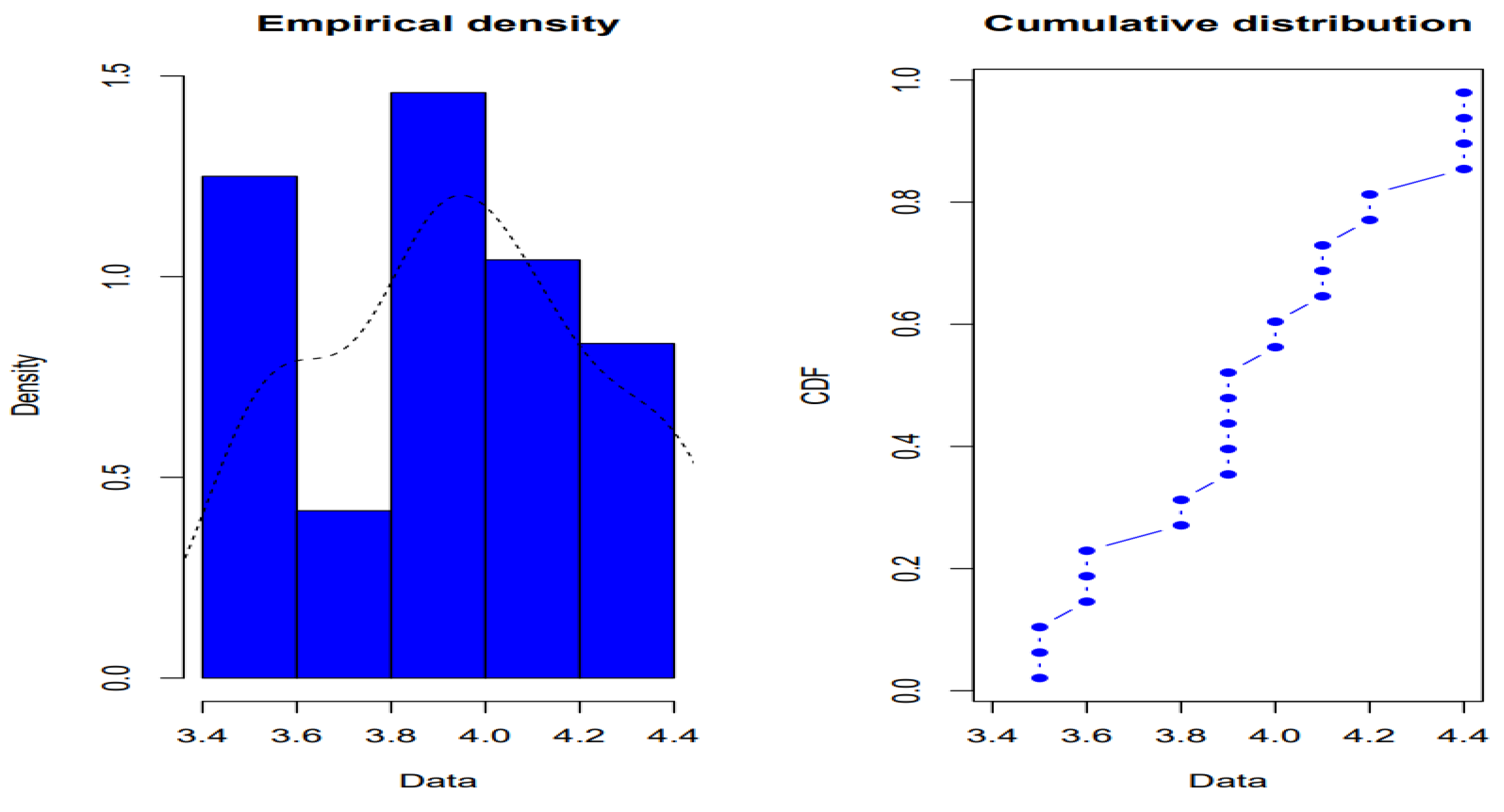
3.4. Results of Empirical Probability
The empirical probability density is composed of two phases: a rising phase from 0.3 to 1.2 and a declining phase from 1.25 to 0.The peak water level with the highest empirical probability densities are between 3.8 meters and 4.0 meters (Figure 5)
Figure 5.
Empirical probability density of annual water level peaks.
3.5. Results of the Fitting to Statistical Distributions
The L-moments estimation method applied to determine the parameters of the three best distributions such as Gumbel, GEV, and GPA fitted to the annual peak water level of Nokoue lake yielded the following results (Table 4, Figure 6, Figure 7, Figure 8, Figure 9) are presented below.
The plots of annual peak water level of Nokoue lake as a function of return period, created on a semi-logarithmic scale, do not perfectly follow the shapes of the various distribution curves. Figure 9 below shows the results of the fitting performed for each of the three best statistical distributions such as Gumbel, GEV, and GPA. The graphical analysis indicates that the scatter plot is best represented by the Gumbel distribution. The result in the root mean square error (RMSE) of the Gumbel distribution is estimated at 0.0724 (Figure 9). It is the smallest value of the observed root mean square error, indicating that the Gumbel distribution best represents the annual peak water level of Nokoue lake. It is important to note that the performance evaluation focused on the ability of different theoretical distributions to replicate the sample of peak water level values for Nokoue lake. For this purpose, cumulative distribution function curves, L-moment diagrams, and Taylor diagrams were constructed to identify the best-fitting distributions. The comparison of the cumulative distribution function of the Gumbel distribution with those of the GEV and GPA distributions fitted to the annual peak water level revealed different root mean square errors (RMSE). The Gumbel distribution performed best, with an RMSE of 0.0724, compared to RMSEs of 0.0754 for the GEV and 0.0761 for the GPA distributions, respectively (Figure 10a, Figure 10b). Recall that the L-moment diagram is a graphical representation of the coefficients of kurtosis against the coefficients of skewness. These were plotted to compare the distributions that align with the sample of annual peak water level for Nokoue lake. This representation showed that the L-moment diagrams of both the Gumbel and GEV distributions closely approximate the annual peak water levels of Nokoue lake (Figure 10d). The Taylor diagram was used to evaluate the root mean square error (RMSE), correlation coefficient, and standard deviation for the generalized extreme value (GEV) distribution applied to the sample of annual peak water level of Nokoue lake. The comparison of these coefficients revealed that the Gumbel model has the highest correlation coefficient, estimated at 97%, and the lowest values of RMSE and standard deviation (), estimated at 1 and 0.45, respectively (Figure 10c).
3.6. Results of the Water Level Peaks Estimates for the Gumbel, GEV, and GPA Distributions
For the preliminary determination of flood quantiles at extreme frequencies and the return period (RP) of the reference flood, the three best distributions were selected based on their superior performance in the model selection tests (Table 5, Table 6). The Gumbel distribution appears to fit the tail of the distribution better. For exceedance probabilities ranging from 0.85 to 0.01, the quantiles estimated with the Gumbel distribution closely approximate the empirical quantiles (Table 5). The quantiles associated with return periods (RP) of 2, 3, 5, 6, 7, 8, 9, 10, 15, 20, 25, 30, 35, 40, 45, 50, 55, 60, 65, 70, 75, 80, 85, 90, 95, and 100 years are provided in Table The reference flood for the Nokoue lake station is the highest recorded quantile value, corresponding to 5.05 m/day with the Gumbel distribution, with an associated return period of 150 years. This implies that the reference flood has a 0.66% chance of occurring annually. The annual peak water level for the 100-year return period is 4.95 m/day. The box plot (Figure 11) shows that most of the annual peak water level of Nokoue lake estimated with the Gumbel distribution are below the mean.
4. Discussion
The standardized water level index for Nokoue lake, ranging from to , allow for the categorization of hydrological thresholds, corresponding respectively to the limited, moderate, significant, and critical hazard classes [25,26,27]. This categorization of hydrological thresholds helps define the extent of flooding in the Nokoue lake watershed. Flood hazard water level thresholds vary according to the risk level, as shown in Figure The analysis of Figure 3 indicates that the periods and were characterized by a high frequency of positive index in the Nokoue lake watershed. This suggests that the study area experienced hydrologically wet conditions, marked by floods during these years. These periods of significant water level increases in the Nokoue lake watershed result from the inflows from the lake's tributaries, combined with excess rainfall over the corresponding periods. This return to a wet state aligns with previous studies conducted in West Africa, specifically in Benin by [25,28], [51] and in Burkina Faso by [26,27] and elsewhere [29,30], [52,53]. The results of the statistical fitting show that for the sample of annual water level peaks of Nokoue lake, the Gumbel, GEV, and GPA distributions are the three best fits for the data. The fitting curves for these three distributions are quite similar. The plot of annual water level peaks against the logarithm of the return period displays a concave shape with indefinite growth. This concavity is dictated by the sign of the shape coefficient for each distribution, which influences the curvature in the distribution tails. Beyond the 10-year return period, the Gumbel distribution shows higher concavity compared to GEV and GPA. From an asymptotic perspective, the Gumbel distribution provided the best fit for the sample, making it the selected model for annual water level peaks. This could be explained by its asymptotic behavior [31]. This could be partly explained by the fact that the Gumbel distribution provides acceptable results when using the robust L-moment estimation method [32,33,34], [35,36,37]. Additionally, it is supported by extreme value theory. The Fisher-Tippett-Gnedenko theorem states that for a series of independent and identically distributed observations following a common distribution , the limit of their linearly normalized maxima as approaches infinity converges toward a Gumbel distribution [38,39], [40,41,42], who studied around thirty hydrometric stations in Wallonia, also demonstrated that the Gumbel distribution was suitable for determining flood flows in 95% of basins when using the annual peak flow method. The authors of this reference [43,44,45,46], [47] demonstrated that the GPA distribution was much more suitable for a series composed of values exceeding a threshold. It confirms that the tail of the GPA distribution is thicker as the value of the parameter increases. Our results corroborate with those of [48,49], [50]. These authors, in their study, demonstrated that the Gumbel distribution was more efficient than the GEV and GPA distributions. They recommended that the estimation of parameters using the maximum likelihood method for the GEV distribution and the generalized Pareto distribution (GPA) can be carried out very effectively and accurately using a global optimization tool that can bypass various local optima.
5. Conclusions
The Gumbel model correctly reproduces the curves of peak flood water heights for Nokoue lake. The return period of the largest flood experienced by Nokoue lake is 150 years. The Gumbel model will be used for the preliminary determination of the peak water heights related to floods in the Nokoue lake watershed. The main limitation of this work lies in the choice of probability distributions and the method of parameter estimation. Indeed, there is no universal and infallible method for choosing the distributions suited to different situations. However, this case study of the Nokoue lake watershed serves as a basis for all flood prevention structures in the Nokoue lake basin and the determination of alert thresholds.
ACKNOWLEDGMENTS
This work is supported in part by the World Bank and the French Development Agency through Centre d’Excellence pour l’Eau et l’Assainissement en Afrique (C2EA) of University of Abomey-Calavi in Benin. The authors would like to thank the reviewers for their constructive comments, which have certainly improved the quality and readability of the article.
Conflicts of interest
The authors declare that there are no conflicts of interest.
References
- S. Yue et P. A. Pilon. Comparison of the power of the test, Mann–Kendall and bootstrap tests for trend detection. Hydrol. Sci. J. 2004,49(1), pp.21 - 38.
- Dabire, N.; Ezin, E.C.;Firmin, A.M. Forecasting Nokoue lagon Water Levels Using Long Short-Term Memory Network. Hydrology journal 2024,.
- Namwinwelbere, D., Eugène, E. C., & Firmin, A. M. Current State of Flooding and Water Quality of Nokoue Lake in Benin (Ouest Africa). European Journal of Environment and Earth Sciences 2022, 3(6), pp.75–81.
- N. Dabire, E.C. Ezin and A.M. Firmin. Water quality index of nokoue lagon prediction using random forest and artificial neural network Int. J. of Adv. Res 2024, pp.610-624.
- N. Dabire, E. C. Ezin and A. M. Firmin. Water Quality Assessment Using Normalized Difference Index by Applying Remote Sensing Techniques: Case of Nokoue lagon. 2024 IEEE 15th Control and System Graduate Research Colloquium (ICSGRC), Shah Alam, Malaysia, 2024, pp.-6, doi:.
- Meylan, P. et Musy, A. Hydrologie fréquentielle. Editions H.G.A Bucarest, 1999, p.413.
- Paturel J. E. et Servat E. Variabilité du régime pluviométrique de l'Afrique de l'Ouest non sahélienne entre 1950 et 1989 : Hydrological Sciences Journal 1998, 43, 921-935.
- Liang Peng and A.H. Welsh. Robust estimation of the generalized pareto distribution. Extremes 2001, 4(1), pp.53–65. [CrossRef]
- Smith R. L Multivariate Threshold Methods. Kluwer, Dordrecht.
- Meylan, P., Favre, A.C, Musy, A. Hydrologie fréquentielle : Une science prédictive. Presses Polytechniques et Universitaires Romandes, 2008, pp.168.
- Édition : Édition du millénaire, p.265.
- Coles S. An Introduction to Statistical Modelling of Extreme Values. Springers Series in Statistics, London, 2001.
- Laborde J.P. Eléments d'hydrologie de surface. L’Université de Nice-Sophia Antipolis, Edition Centre National de la Recherche Scientifique (C.N.R.S), 2000, pp.137.
- Hosking J.R.M. and J.R. Wallis. Parameter and quantile estimation for the generalized pareto distribution. Technometrics 1987, 29(3), pp.339–349.
- Kluppelberg C. and A. Bivariate extreme value distributions based on polynomial dependence ¨ functions. Math Methods Appl Sci 2006, 29(12),pp.1467–1480. [CrossRef]
- B. T. Goula, A. Konan, T. Brou, Y. Issiaka, S. V. Fadika et B Srohourou. Estimation des pluies exceptionnelles journalières en zone tropicale: cas de la Côte d'Ivoire par comparaison des lois log normale et de Gumbel. Hydrological sciences journal 2007, 52 (1), pp.49 -67.
- Habibi, M. Meddi et A. Boucefiane. Analyse fréquentielle des pluies journalières maximales : Cas du Bassin Chott-Chergui. Nature et Technology 2013, (8), pp.41.
- N. Soro, T. Lasm, B. H. Kouadio, G. Soro, K. E. Ahoussi. Variabilité du régime pluviométrique du Sud de la Côte d'Ivoire et son impact sur l'alimentation de la nappe d'Abidjan. Rev. Sud Sciences et technologies 2006, (14), pp.30-40.
- Mises, R., von. La distribution de la plus grande de n valeurs. Selected papers, 1954,2, pp.271-294.
- Bortot P. and S. Coles. The multivariate gaussian tail model: An application to oceanographic data. Journal of the Royal Statistical Society. Series C: Applied Statistics 2000, 49(1), pp.31–49. [CrossRef]
- Coles, J. Heffernan, and J. Tawn. Dependence measures for extreme value analyses. Extremes 1999, 2(4), pp.339–365.
- Fisher R.A. and L.H. Tippett. Limiting forms of the frequency distribution of the largest or smallest member of a sample. In Proceedings of the Cambridge Philosophical Society 1928, 24, pp.180–190. [CrossRef]
- Fréchet M. Sur la loi de probabilité de l’écart maximum. Annales de la Société polo-naise de Mathématique 1927, Cracovie.
- Gumbel É.J. Statistical theory of extreme values and some practical applications. National Bureau of Standards 1954, Washington. [CrossRef]
- Jenkinson A. F. The frequency distribution of the annual maximum (or minimum) values of meteorological events. Quaterly Journal of the Royal Meteorological Society 1955, 81,pp.158–172.
- D. H. Koumassi. Risques hydroclimatiques et vulnérabilité des écosystèmes dans le bassin-versant de la Sota. Thèse de Doctorat de l’Université d’Abomey-Calavi, 2014, pp.244.
- T. P. Zoungrana. Les stratégies d’adaptation des producteurs ruraux à la variabilité climatique dans la cuvette de Ziga, au centre du Burkina Faso". Anales de l’université de Ouagadougou – Série A, Vol. 011, 2010, pp.585 -606.
- S. Rouamba. Variabilité climatique et accès à l’eau dans les quartiers informels de Ouagadougou. Thèse de doctorat de géographie, Université Ouaga I Pr Joseph Ki-Zerbo, 2017, pp.283.
- V. S. H. Totin, E. amoussou, L. Odoulami, M. boko, B. A. Blivi. Seuils pluviométriques des niveaux de risque d’inondation dans le bassin de l’Ouémé au Benin (Afrique de l’ouest) . XXIXe Colloque de l’Association Internationale de Climatologie, Lausanne -Besançon, 2016, pp.369 - 374.
- M. Hache, L. Perreault, L. Remillard et B. Bobee. Une approche pour la sélection des distributions statistiques: application au bassin hydrographique du Saguenay-Lac St-Jean. Canadian Journal of Civil Engineering 1999, 26 (2), pp. 216 -225.
- Habibi, M. Meddi et A. Boucefiane. Analyse fréquentielle des pluies journalières maximales : Cas du Bassin Chott-Chergui. Nature et Technology, 2013, 3(8), pp.41.
- Jowitt, P.W. The extreme-value type 1 and the principal of maximums entropy. J. Hydrol 1979, 4(2), pp.23-38.
- Juarez S.F. and W.R. Schucany. Robust and efficient estimation for the generalized pareto distribution. Extremes 2004, 7(3), pp.237–251. [CrossRef]
- Pickands J. Multivariate extreme value distributions. In Proceedings 43rd Session International Statistical Institute 1981.
- Pickands J. III. Statistical inference using extreme order statistics. Annals of Statistics, 1975, 3, pp.119–131.
- CIEH. Courbes hauteur de pluie-fréquence Afrique de l‘Ouest et Centrale pour des pluies de duràe 5 mn à 24 h. 1984.
- Christophe Ancey. Risques hydrologiques et aménagement du territoire. École Polytechnique Fédérale de Lausanne, Ecublens, CH-1015 Lausanne, Suisse,2011.
- Cunnane C. Note on the poisson assumption in partial duration series model. Water Resour Res, 1979, 15(2), pp.489–494. [CrossRef]
- Matthew J. Purvis, Paul D. Bates, Christopher M. Hayes. A probabilistic methodology to estimate future coastal flood risk due to sea level rise,Coastal Engineering 2008, 5(12), pp.1062-1073. [CrossRef]
- Courtney M. Thompson, Tim G. Frazier, Deterministic and probabilistic flood modeling for contemporary and future coastal and inland precipitation inundation, Applied Geography 2014, 50,. [CrossRef]
- ,pp.1-14.
- Roman Krzysztofowicz. Probabilistic flood forecast: Exact and approximate predictive distributions, Journal of Hydrology 2014, 5(17), pp.643-651. [CrossRef]
- Pascal Lardet, Charles Obled. Real-time flood forecasting using a stochastic rainfall generator,. [CrossRef]
- Journal of Hydrology1994, 1(6), pp. 391-408.
- Shien-Tsung Chen, Pao-Shan Yu. Real-time probabilistic forecasting of flood stages,. [CrossRef]
- Journal of Hydrology2007, 3(4), pp.63-77.
- Roman Krzysztofowicz. The case for probabilistic forecasting in hydrology,. [CrossRef]
- Journal of Hydrology2001, 2(4), pp. 2-9.
- Kupfer, S., MacPherson, L. R., Hinkel, J., Arns, A., & Vafeidis, A. T. A comprehensive probabilistic flood assessment accounting for hydrograph variability of ESL events. Journal of Geophysical Research: Oceans, 2024 , pp.129. [CrossRef]
- Karl-Erich Lindenschmidt, Prabin Rokaya, Apurba Das, Zhaoqin Li, Dominique Richard. A novel stochastic modelling approach for operational real-time ice-jam flood forecasting, Journal of Hydrology 2019, 5(7), pp.381-394. [CrossRef]
- S. I. Resnick. Extreme Values, Regular Variation and Point Processes. New–York: Springer–Verlag, 1987.
- R Development Core Team. R: A Language and Environment for Statistical Computing. R Foundation for Statistical Computing, Vienna, Austria, 2006.
- C. Kluppelberg and A. May. Bivariate extreme value distributions based on polynomial dependence ¨ functions. Math Methods Appl Sci, 2006, 29(12), pp.1467–1480. [CrossRef]
- M. Falk and R.-D. Reiss. On pickands coordinates in arbitrary dimensions. Journal of Multivariate Analysis, 2005, 92(2), pp.426–453. [CrossRef]
- S. Coles. An Introduction to Statistical Modelling of Extreme Values. Springer Series in Statistics. Springers Series in Statistics, London, 2001.
- Izinyon, N. Ihimekpen et G.E. Igbinoba. Analyse de la fréquence des inondations du bassin versant de la rivière Ikpoba à Benin City à l’aide de la distribution Log Pearson de type III. Journal des tendances émergentes en génie et en sciences appliquées 2011, 2(1), pp.50–55.
- .Mujere N. Flood frequency analysis using the Gumbel distribution. Int J Comput Sci Eng 2011, 3(7), pp.2774–2788.
- Mukherjee MK. Flood frequency analysis of River Subernarekha, India, using Gumbel’s extreme value distribution. Int J Comput Eng Res 2013, 3(7), pp.12–19.
- Singo LR, Kundu PM, Odiyo JO, Mathivha FI, Nkuna TR. Flood frequency analysis of annual maximum stream flows for Luvuvhu River catchment, Limpopo Province, South Africa. University of Venda, Department of Hydrology and Water Resources, Thohoyandou, South Africa 2013, pp. 1–9.
- E. Haque. Flood Frequency Analysis of the Kaljani River of West Bengal: A Study in Fluvial Geomorphology. In: Das, J., Halder, S. (eds) New Advancements in Geomorphological Research. Geography of the Physical Environment 2024 Springer, Cham,.
Figure.
Location of the study area.
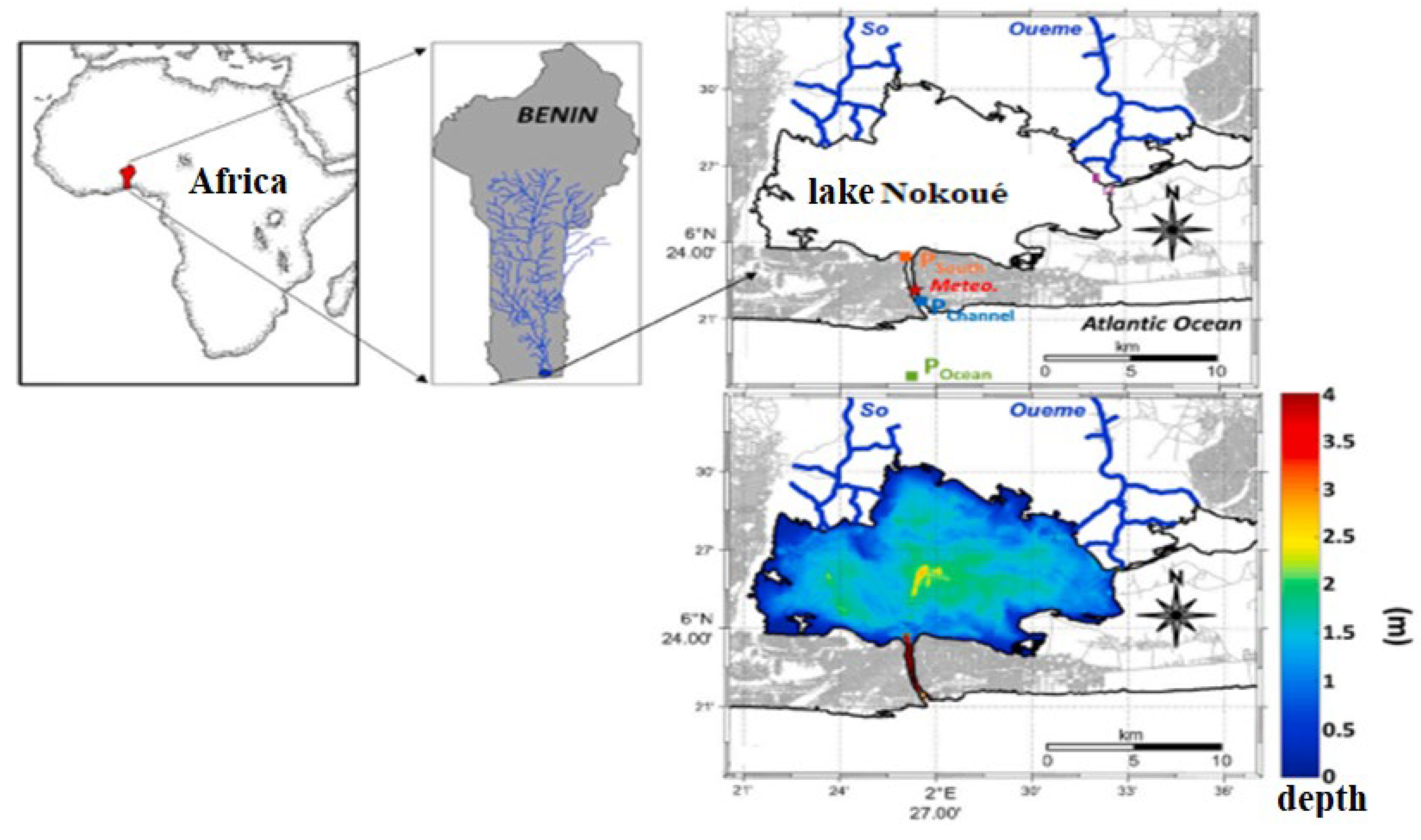
Figure 2.
Annual water level peaks.
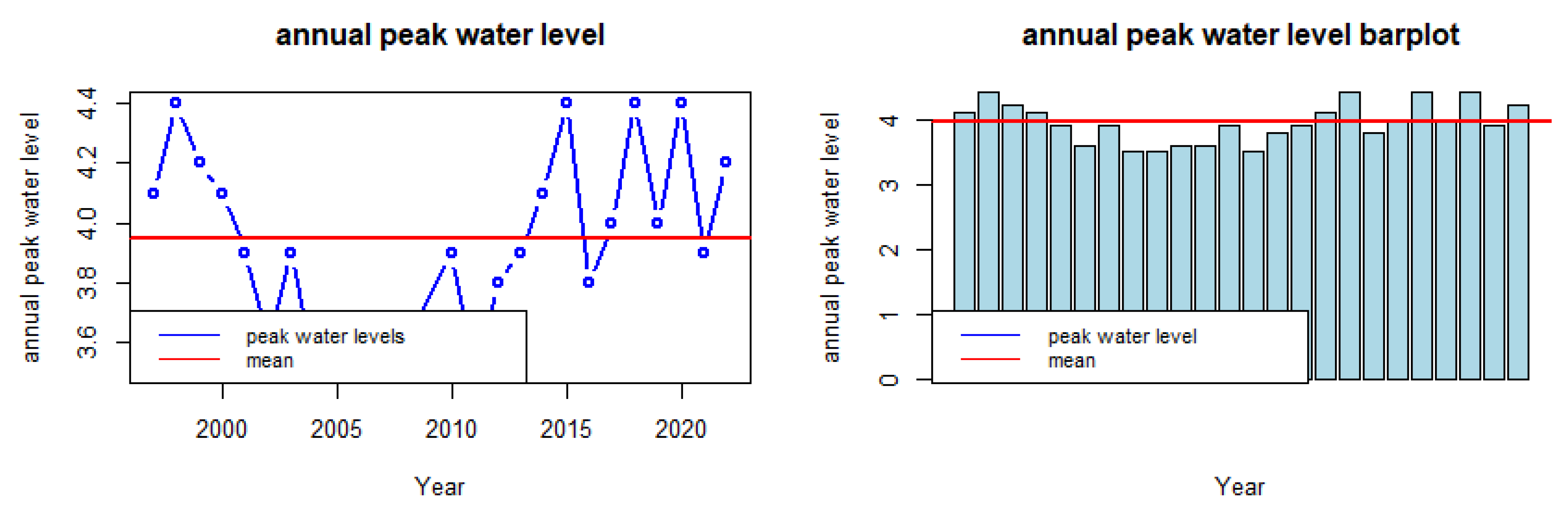
Figure 3.
Standardized index of water level peak.
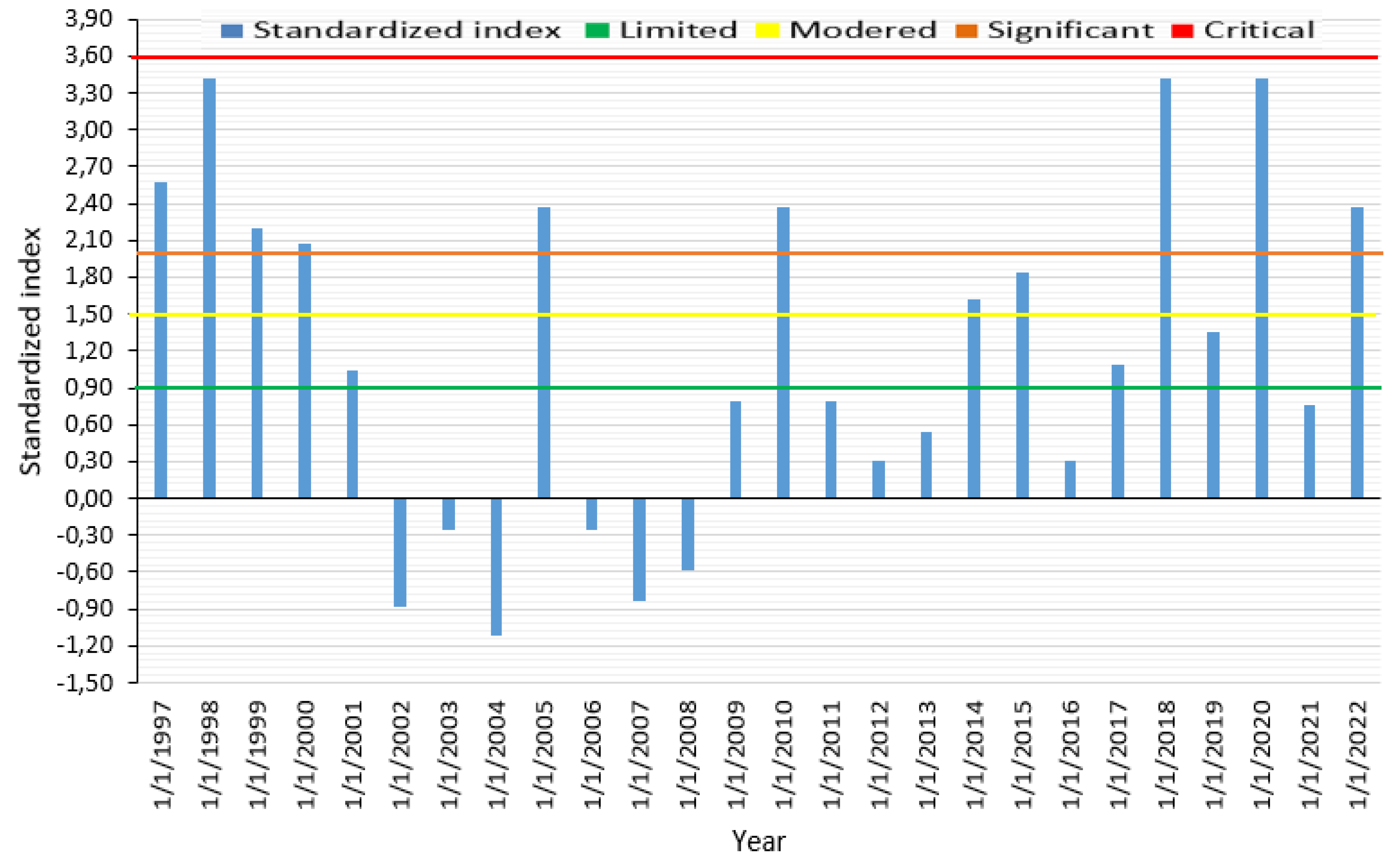
Figure 4.
Water level Peak thresholds for Nokoue lake.
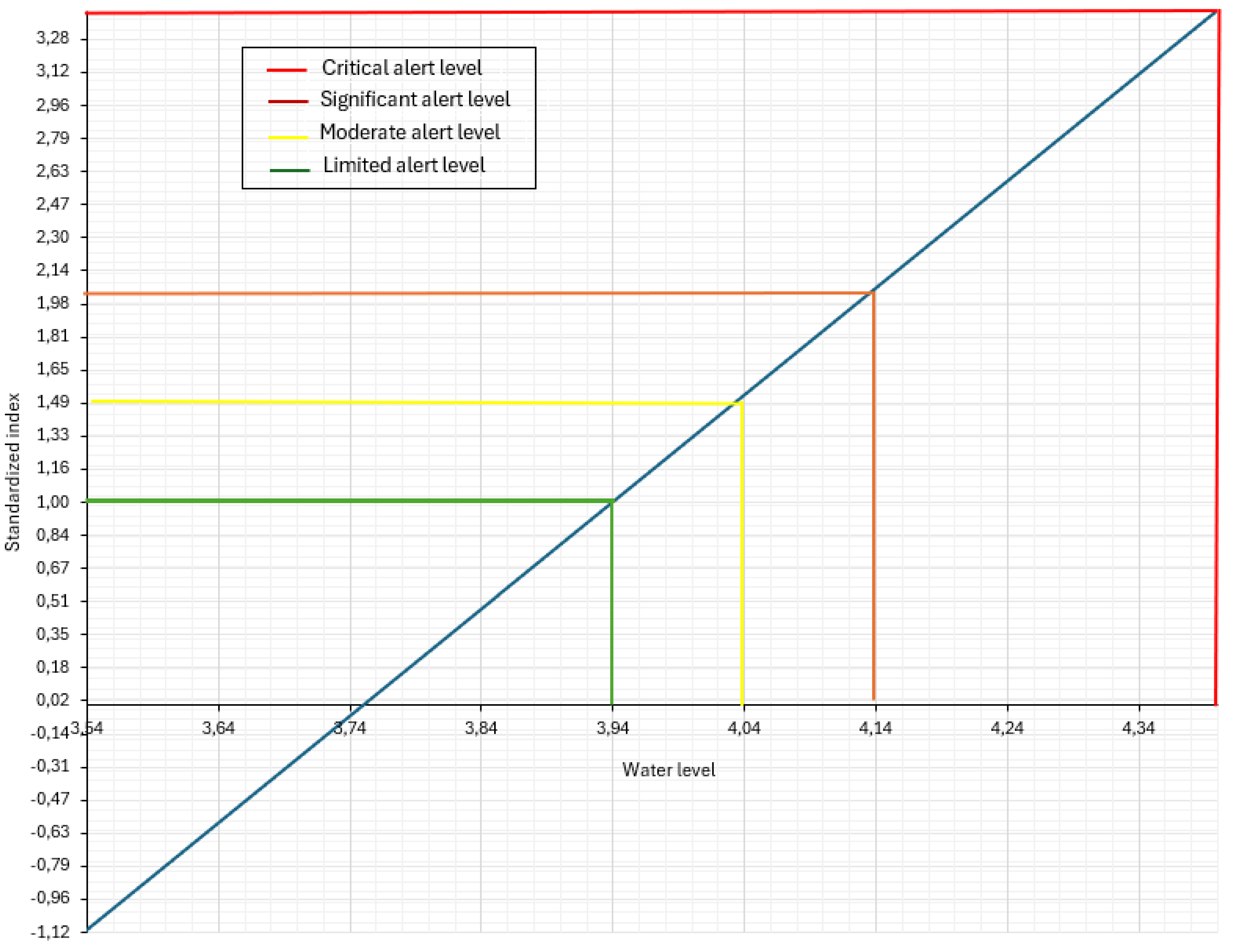
Figure 6.
Parameters of the Generalized Extreme Value (GEV) distribution.
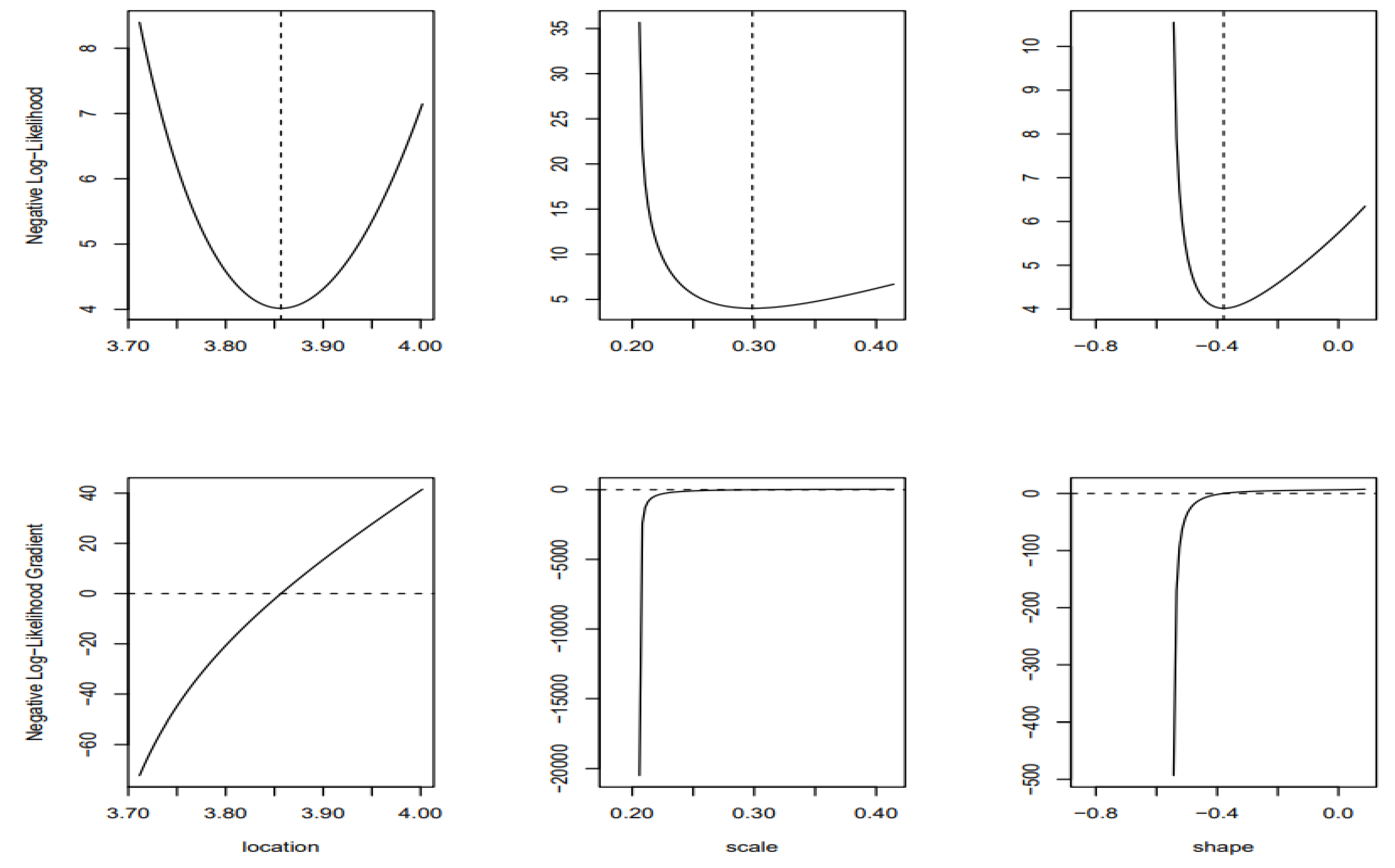
Figure 7.
Parameters of the Gumbel distribution.
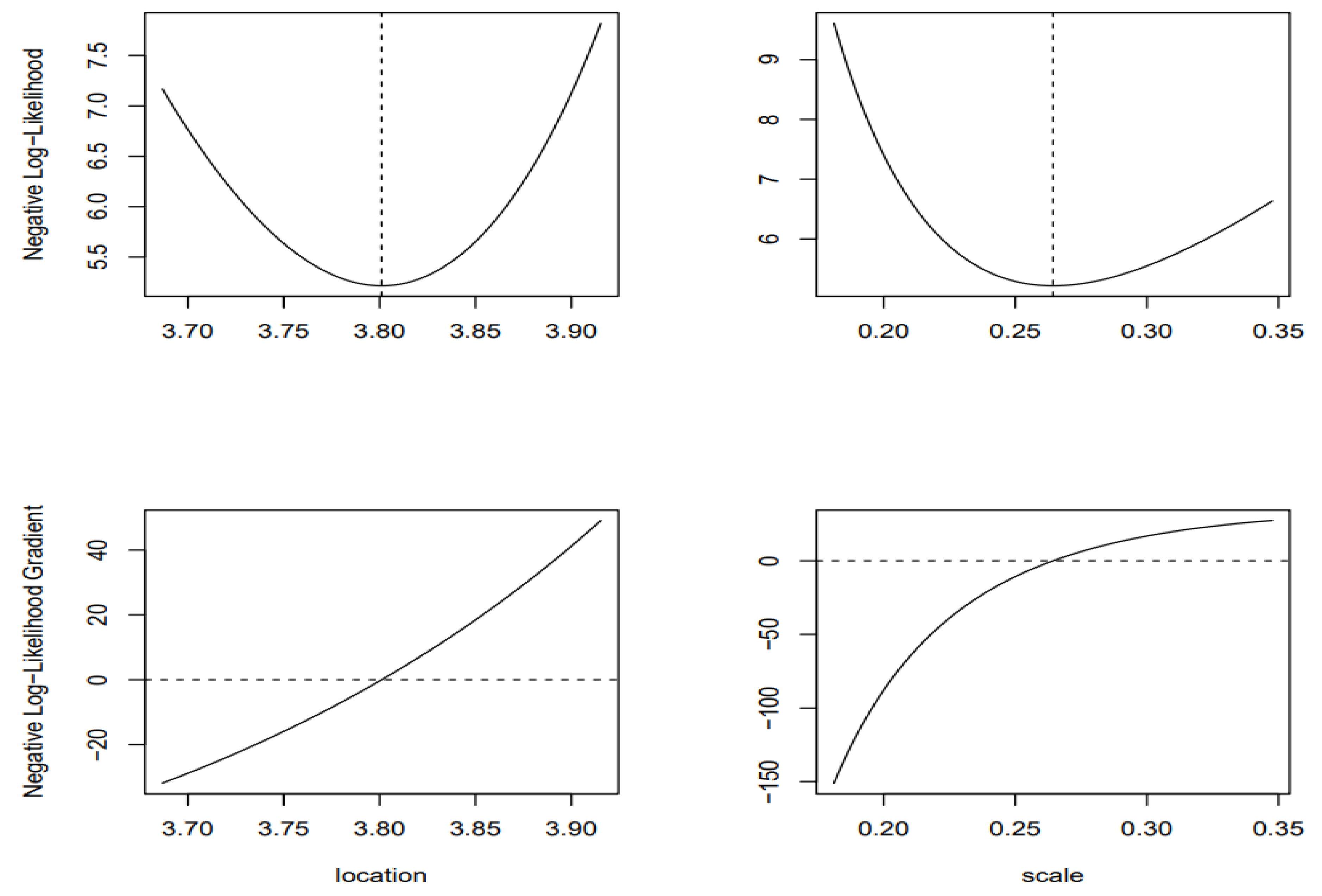
Figure 8.
Parameters of the Generalized Pareto (GPA) distribution.
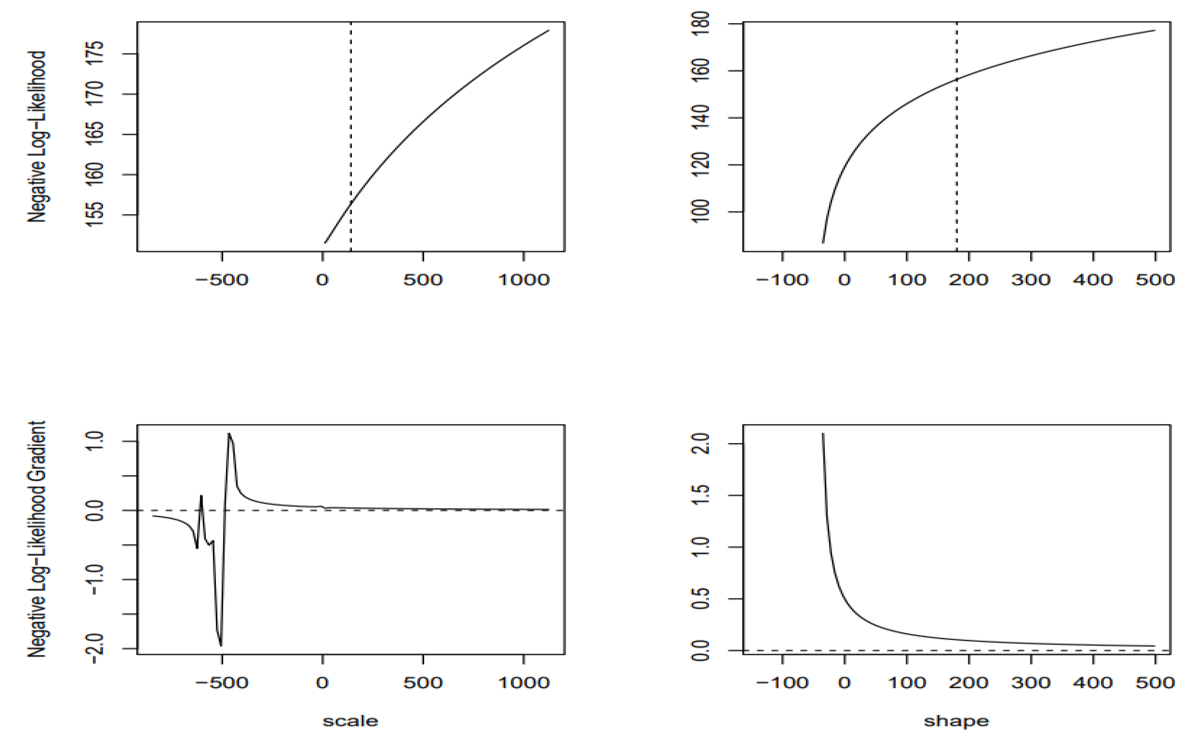
Figure 9.
Comparison of the quality of distribution fittings.
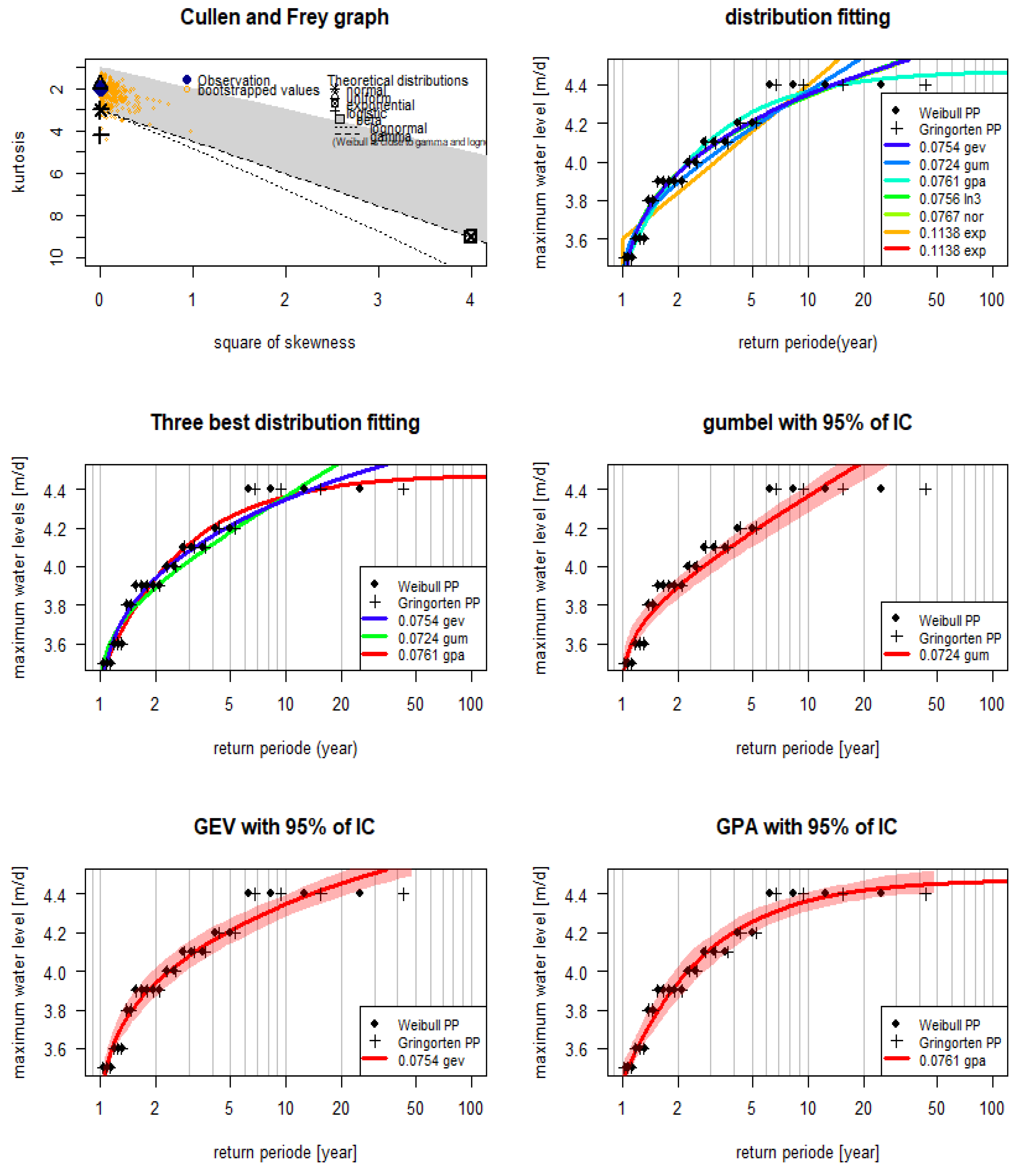
Figure 10.
Performance of distributions in the frequency analysis of annual peak water level of Nokoue lake: (a) Probability density function; (b) Cumulative distribution function; (c) Taylor diagram; and (d) L-moment diagrams..
Figure 10.
Performance of distributions in the frequency analysis of annual peak water level of Nokoue lake: (a) Probability density function; (b) Cumulative distribution function; (c) Taylor diagram; and (d) L-moment diagrams..
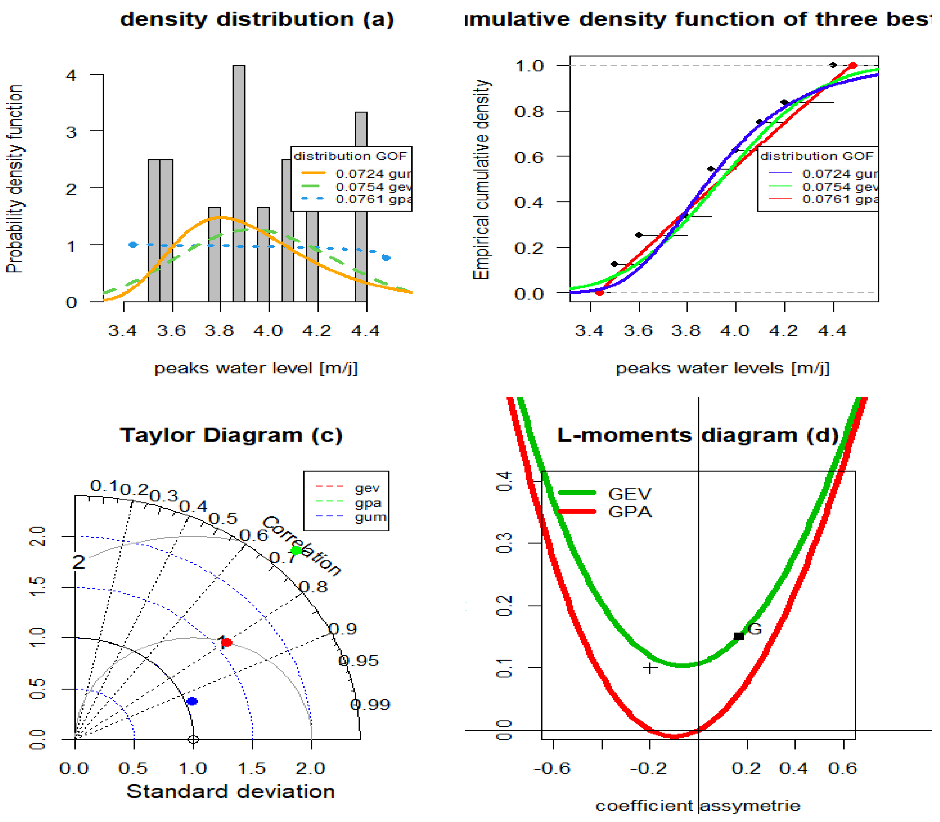
Figure 11.
Box plots of the estimated quantiles from the distribution.
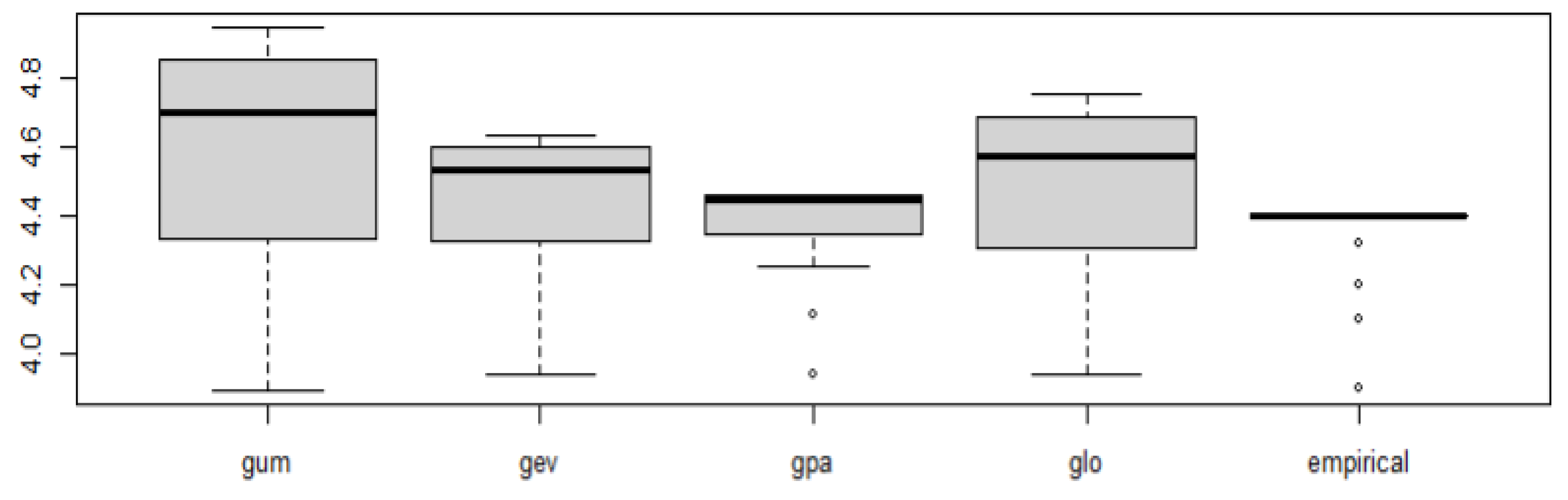

Table 1.
Categorization of flood risk alert thresholds.
| Risk Level | Risk categories |
|---|---|
| Critical | ≥ 2.0 |
| Significant | < 2 |
| Moderate | < 1.5 |
| Limited | < 1 |
Table 2.
Summary statistics of annual peak water level values.
| min | 25% | 50% | 75% | max | Standard diviation |
|---|---|---|---|---|---|
| 3.5 | 3.75 | 3,95 | 4.13 | 4,4 | 0.2 |
Table 3.
Results of the statistical tests.
| Statistical tests | p-value | Status |
|---|---|---|
| independance | 0.12 | accepted |
| Homogeneity | 0.14 | accepted |
| Stationarity | 0.14 | accepted |
Table 4.
Results of the parameters for the Gumbel, GEV, and GPA distributions.
| Statistical distributions | Parameters | ||
|---|---|---|---|
| lois de Gumbel | 3.80 0.25 | ||
| lois GEV | 0.30 0.3 | 0.27 | |
| Lois GPA | 3.43 1.003 | 0.96 | |
Table 5.
Exceedance probability associated with the estimated quantiles and the RMSE of the distributions.
Table 5.
Exceedance probability associated with the estimated quantiles and the RMSE of the distributions.
| 0.85 | 0.75 | 0.5 | 0.25 | 0.2 | 0.1 | 0.01 | RMSE | |
|---|---|---|---|---|---|---|---|---|
| Gumbel | 3.642573 | 3.720708 | 3.893353 | 4.112385 | 4.175660 | 4.362572 | 4.947841 | 0.07238795 |
| GEV | 3.625181 | 3.732998 | 3.941547 | 4.156290 | 4.209517 | 4.347250 | 4.636763 | 0.07543231 |
| GPA | 3.585419 | 3.686597 | 3.941998 | 4.202556 | 4.255658 | 4.363591 | 4.465037 | 0.07610624 |
| Empirical | 3.598333 | 3.683333 | 3.900000 | 4.158333 | 4.200000 | 4.400000 | 4.400000 | |
| Quantiles mean | 3.592593 | 3.663426 | 3.900000 | 4.134954 | 4.200000 | 4.400000 | 4.400000 |
Table 6.
Quantile values associated with return periods.
| RP.2 | RP.3 | RP.6 | RP.7 | RP.8 | RP.9 | RP.10 | |
|---|---|---|---|---|---|---|---|
| Gumbel | 3.893353 | 4.026908 | 4.225984 | 4.267789 | 4.303554 | 4.334811 | 4.362572 |
| GEV | 3.941547 | 4.078418 | 4.249350 | 4.280847 | 4.306698 | 4.328494 | 4.347250 |
| GPA | 3.941998 | 4.114921 | 4.291336 | 4.316985 | 4.336328 | 4.351446 | 4.363591 |
| Empirical | 3.500000 | 3.900000 | 4.200000 | 4.322222 | 4.400000 | 4.400000 | 4.400000 |
| Q mean | 3.500000 | 3.900000 | 4.200000 | 4.270988 | 4.384127 | 4.400000 | 4.400000 |
| RP.15 | RP.20 | RP.30 | RP.35 | RP.40 | RP.45 | RP.50 | |
| Gumbel | 4.468026 | 4.541862 | 4.645004 | 4.684007 | 4.717721 | 4.747411 | 4.773935 |
| GEV | 4.413629 | 4.455843 | 4.509497 | 4.528292 | 4.543918 | 4.557220 | 4.568751 |
| GPA | 4.400367 | 4.419004 | 4.437885 | 4.443340 | 4.447454 | 4.450669 | 4.453252 |
| Empirical | 4.400000 | 4.400000 | 4.400000 | 4.400000 | 4.400000 | 4.400000 | 4.400000 |
| Q mean | 4.400000 | 4.400000 | 4.400000 | 4.400000 | 4.400000 | 4.400000 | 4.400000 |
| RP.55 | RP.60 | RP.70 | RP.75 | RP.80 | RP.85 | RP.90 | |
| Gumbel | 4.797905 | 4.819768 | 4.858464 | 4.875768 | 4.891948 | 4.907140 | 4.921459 |
| GEV | 4.578894 | 4.587922 | 4.603390 | 4.610103 | 4.616268 | 4.621961 | 4.627242 |
| GPA | 4.455374 | 4.457148 | 4.459948 | 4.461073 | 4.462060 | 4.462933 | 4.463711 |
| Empirical | 4.400000 | 4.400000 | 4.400000 | 4.400000 | 4.400000 | 4.400000 | 4.400000 |
| Q mean | 4.400000 | 4.400000 | 4.400000 | 4.400000 | 4.400000 | 4.400000 | 4.400000 |
| RP.95 | RP.100 | ||||||
| Gumbel | 4.934999 | 4.947841 | |||||
| GEV | 4.632162 | 4.636763 | |||||
| GPA | 4.464408 | 4.465037 | |||||
| Empirical | 4.400000 | 4.400000 | |||||
| Q mean | 4.400000 | 4.400000 |
Disclaimer/Publisher’s Note: The statements, opinions and data contained in all publications are solely those of the individual author(s) and contributor(s) and not of MDPI and/or the editor(s). MDPI and/or the editor(s) disclaim responsibility for any injury to people or property resulting from any ideas, methods, instructions or products referred to in the content. |
© 2024 by the authors. Licensee MDPI, Basel, Switzerland. This article is an open access article distributed under the terms and conditions of the Creative Commons Attribution (CC BY) license (http://creativecommons.org/licenses/by/4.0/).
Copyright: This open access article is published under a Creative Commons CC BY 4.0 license, which permit the free download, distribution, and reuse, provided that the author and preprint are cited in any reuse.


