
Submitted:
31 October 2024
Posted:
01 November 2024
You are already at the latest version
Abstract
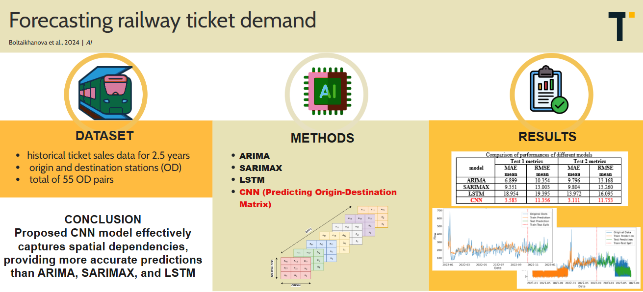
This research paper investigates methodologies for forecasting the demand for railway tickets, a crucial aspect of optimizing resource allocation, enhancing service quality, and increasing revenue in railway transportation systems. The study explores various time series analysis techniques, including ARIMA, SARIMAX, and neural networks such as LSTM and CNN, to predict ticket demand. Railway ticket sales data spanning several years was utilized to train and validate the models. The performance of each model was evaluated based on key metrics like Mean Absolute Error (MAE), and Root Mean Squared Error (RMSE). Demand is usually defined in Origin-Destination (OD) matrices, which represent movements from the origin station to the destination station for all OD pairs. The proposed CNN model predicts the OD matrix, whereas other models predict demand for each OD pair separately. Findings indicate that the CNN model gives more accurate predictions compared to ARIMA, SARIMAX, and LSTM models. Hence, interdependencies between various OD pairs allow for a more holistic and accurate prediction model.
Keywords:
railway system
; demand forecasting
; revenue management
; machine learning
; neural networks
; time series
; ARIMA
; SARIMAX
; origin-destination (OD) pairs
; OD matrix
; CNN
1. Introduction
Forecasting demand for railway passenger transportation is an important tool for decision-making in the sphere of railway transportation. It allows carriers to assess the market potential, identify the most promising areas, and develop an effective revenue management model. The revenue management system involves dynamic pricing through capacity management. It entails intelligently allocating offered seats to fare buckets based on demand at the origin-destination (OD) stations. This system operates by opening or closing fare buckets based on the rules set by the carrier as part of its revenue management strategy. Consequently, tickets in distinct fare buckets are marketed at varying rates. Usually, when tickets from the cheapest fare box sell out, that box closes, and the next box opens - with higher fares and more services [1]. Typically, cost-conscious passengers are willing to purchase more affordable tickets in advance, while corporate travelers are willing to pay a premium for last-minute bookings. Carrier companies worldwide monitor demand and dynamically respond by opening low-cost options to promote purchases or closing them earlier if demand is excessive. Usually, fares within segments remain constant, although they can be influenced by external factors such as weather conditions, competitive air and road transport markets, seasonality, and holiday periods [2].
Demand forecasting for railroad tickets holds significant importance due to its multifaceted benefits. Firstly, it can enhance revenue by enabling companies to optimize their pricing strategies, thereby providing passengers with more attractive conditions. Secondly, it aids in cost reduction by allowing carriers to utilize their resources more efficiently; for instance, through the optimization of train schedules and the allocation of rolling stock. Lastly, demand forecasting contributes to improving the quality of passenger service, as it enables carriers to accurately predict passenger needs and offer more convenient and comfortable transportation options.
Paper organization
The remainder of this paper is structured as follows: Section 2 provides a review of the existing literature on ticket demand prediction models. Section 3 details the methodology employed in this study, along with an in-depth analysis of the dataset. Section 4 presents the study's findings and offers a discussion of the results. Finally, Section 5 concludes the paper by summarizing its key findings and suggesting areas for future research.
2. Background and Related works
Currently, there are numerous studies investigating demand models, ranging from theoretical advancements in general cases to practical applications in private research. In the literature, various studies have employed machine learning, artificial neural networks, and statistical methods to predict passenger transportation demand. For instance, ARIMA (autoregressive integrated moving average) model was utilized for demand forecasting, alongside an exponential error smoothing model [3]. This research leveraged national-level data on rail passenger traffic in Poland from 2014 to 2019, concluding that the ARIMA model outperformed the exponential error smoothing model.
Similarly, the SARIMA (seasonal autoregressive integrated moving average) model was applied to forecast passenger transportation demand within the Serbian railway network [4]. This model developed using historical data from monthly passenger counts, demonstrated high accuracy in predicting demand with seasonal variations. However, it is noteworthy that this model only incorporated historical demand data, neglecting other potentially influential factors such as demographics, class preferences, and the timing of ticket purchases.
In other research, the influence of search queries on the accuracy of forecasting the demand for railroad tickets was investigated [5]. The demand for tickets is calculated as the difference between the maximum and the remaining number of seats before the train departure. The sum of demand by departure dates in a certain period is used for forecasting. Time series forecasting techniques such as ARIMA, SARIMA, and LSTM are applied in the paper. Experiments include forecasting variants with and without predictors (number of search queries).
The origin - destination flow was predicted in urban rail transit using a sophisticated CAS-CNN model [6]. The proposed model includes a split convolutional neural network for data compression, a channel-wise attention mechanism for feature extraction, and an inflow/outflow mechanism for combining outputs.
Statistical methods and machine learning algorithms were applied to forecast the demand for passenger rail transportation [7]. In line-by-line analysis, the simple averaging method shows better overall results than regression analysis. When analyzing and forecasting demand by railway stations, the decision tree method shows the best result among all including artificial neural networks.
Demand prediction for intercity bus tickets in Nairobi for 14 destinations is published in open source [8]. Three types of regression algorithms are used to solve the problem: random forest, gradient boosting, and extreme gradient boosting. Hyperparameter tuning and identification of important features have been conducted for each algorithm. As a result of the comparative analysis, the extreme gradient boosting algorithm shows the best result with an accuracy of about 86%.
The objective of the current study is to predict railway ticket demand based on the previous ticket sales data, therefore time series forecasting methods are considered in the study.
3. Methodology
a.Dataset
The models utilized data on passenger railway sales spanning the last 2.5 years (2021, 2022, and 2023) across Kazakhstan, provided by the railway ticket sales agent Nur-Kassa LLP. The dataset includes information on the date of ticket purchase, the origin and destination stations, and the date of train departure, encompassing a total of 55 OD pairs. The top 10 most popular OD pairs, along with the number of tickets sold during the period from 2021 to 2023, are presented in Table 1.
According to the ticket sales data, the most popular route is Almaty – Astana. The three graphs below (Figure 1, Figure 2 and Figure 3) illustrate the number of tickets sold for the Almaty-Astana route by months across the years 2021, 2022, and 2023. The number of tickets sold in 2021 fluctuates throughout the year. There is a noticeable peak in December, where the number of tickets exceeds 17 000, while the other months maintain relatively stable sales, ranging between 5 000 and 10 000. In 2022 ticket sales are generally higher compared to 2021, with the majority of months showing sales between 25 000 and 30 000 tickets. The highest sales are observed in July, August, and December. Conversely, 2023 shows a significant decline in ticket sales as the year progresses.
Figure 4 - Figure 6 illustrate ticket sales for Almaty – Astana route versus the number of days before departure for the years 2021, 2022, and 2023. Across all three years, ticket sales increase as the departure date approaches. Additionally, there is a notable rise in ticket sales approximately 42 to 45 days before departure in 2022 and 2023.
b.Predicting Timeseries using ARIMA and SARIMAX models
In this study, both ARIMA (AutoRegressive Integrated Moving Average) and SARIMAX (Seasonal AutoRegressive Integrated Moving Average with eXogenous variables) models were utilized to forecast ticket sales. The ARIMA model, a well-established statistical method, captures the linear dependencies in the time series data, providing a robust framework for short-term predictions by analyzing historical ticket sales data to identify underlying patterns and trends. The model is mathematically expressed as ARIMA(p, d, q), where p is the order of the autoregressive part (AR), d is the degree of differencing, and q is the order of the moving average part (MA). The equation for an autoregressive and moving average parts are presented in Eq1 and Eq2 subsequently [9]:
where is the predicting value, , and are AR coefficients, , and are MA coefficients, C is a constant and is an error term. Differencing term (d) is used to convert non-stationary time series to stationary and shows the number of times the data have had past values subtracted.
The SARIMAX model extends the model by incorporating seasonal effects and exogenous variables such as holidays, special events, and weather conditions, which are crucial for more accurate forecasting in the context of railway travel. Equations for the SARIMAX model are shown in Eq3 [10].
where and are additional sets of AR and MA components and term stands for exogenous variables.
c.Predicting Timeseries Using Long Short-Term Memory Network
Predicting railway ticket demand using Long Short-Term Memory (LSTM) networks offers a powerful approach to capturing complex temporal dependencies and patterns in ticket sales data. LSTM, a type of recurrent neural network (RNN) designed to overcome the vanishing gradient problem, is particularly effective in modeling time series data due to its ability to retain long-term information [11]. The architecture of the model consists of two LSTM layers with 25 neurons in each and two Dense layers with 10 and 1 neurons (Figure 7). Time step is equal to 7 days by revealing seasonal periodicity in the seasonality test conducted for the SARIMAX model.
d.Predicting Origin-Destination Matrix Using Convolutional Neural Network
The origin-destination matrix is a 3D array that represents the flow of passengers between various locations during a particular period. The flows between different OD pairs are often interdependent due to shared routes and transit hubs in the railway transportation system. By predicting the entire OD matrix, models can learn and exploit these spatial dependencies and interactions. This holistic approach allows for capturing patterns that may be missed when considering each OD pair in isolation and can lead to better accuracy [6]. The structure of the created OD matrix for 55 OD pairs is shown in Figure 8, where aij is the number of sold tickets for origin station i and destination station j. Passenger flow for the previous 7 days was considered in the model.
CNN for predicting OD matrix can be useful for handling spatial dependencies and capturing complex travel patterns. CNNs traditionally used in image processing. In the context of the research task, each element of the OD matrix can be treated as a pixel in an image, allowing the CNN to process the entire matrix as a 3D grid. The methodology involves constructing a CNN architecture with a 2D convolutional layer followed by a pooling layer to reduce dimensionality and extract relevant features and dense layers. Additionally, Dropout is added to overcome overfitting. The output layer is designed to predict the flow values in the OD matrix (Figure 9).
e. Key Performance Indicators
Mean Squared Error (MSE) and Root Mean Squared Error (RMSE) were computed to assess the performance of each model. The equations for MSE and RMSE are given in Eq. (4) and Eq. (5), which represent the actual demand value and denote the predicted value.
To evaluate the prediction quality, two distinct tests were conducted:
i.Test 1 comprised data from the year 2022, with 80% of the data (January to October) used for training and 20% (November to December) for testing.
ii.In the second test (Test 2), the dataset included data from January 2021 to August 2023, with models trained on 65% of the data (January 2021 to August 2022) and tested on the remaining 35% (September 2022 to August 2023). section.
4. Results and Discussion
a.ARIMA and SARIMAX models result
Before fitting the ARIMA and SARIMAX models, the Augmented Dickey-Fuller (ADF) test was conducted to check the stationarity of the demand time series for each OD pair. The results of the ADF test for the 10 popular OD pairs are presented in Table 2.
Non-stationary time series were transformed to stationary by applying differencing. The optimal values for AR, differencing, and MA orders (p, d, q) for the ARIMA model, as well as the AR, differencing, and MA orders (p, d, q) and their seasonal counterparts (P, D, Q) for the SARIMAX model, were determined using the pmdarima library. The seasonal order (S) was identified by decomposing the time series into trend, seasonal, and residual components and calculating the difference between the two minima and two maxima within the seasonal component. As described above procedure was applied to each OD pair. Results revealed that the seasonality is typically 7 days, however, some time series show a seasonality of 0 or 14 days.
ARIMA and SARIMAX models' performance for predicting demand for Almaty – Astana route during November-December 2022 (first test) is illustrated in Figure 10. The green line represents the ARIMA model's predictions. It shows a smoother trend compared to the actual test data, indicating the model’s tendency to generalize and smooth out variations. ARIMA model does not capture the local fluctuations seen in the test data. The red line represents the SARIMAX model's predictions. This model appears to follow the test data more closely, capturing the variations better than the ARIMA model.
On the other hand, when predicting demand for the longer period (September 2022 to August 2023, second test), both models perform poor (Figure 11). ARIMA and SARIMAX models provide a relatively flat forecast that fail to capture the sharp decline and subsequent stabilization in the actual test data.
b.LSTM model result
LSTM model expects input data to be a 3D tensor. The dataset was transformed into a 3D array with shapes (357, 7, 1) for test 1 and (948, 7, 1) for test 2, where the first dimension stands for the number of samples (days), the second dimension is the time step and last dimension is the number of features. The model architecture and the choice of time step (7 days) are described in the Methodology sector.
The predicted demand for Almaty – Astana route is shown in Figure 12 (test 1) and Figure 13 (test 2). According to Figure 12 LSTM model captured the general pattern and variability in the training and testing data. When predicting demand for September 2022 to August 2023 (Figure 13) LSTM model was able to predict rapid decline and subsequent stabilization of the demand. Overall, in forecasting demand for the Almaty–Astana route, the LSTM model more effectively captures the peaks and troughs compared to the ARIMA and SARIMAX models.
The model was trained in 10 epochs. Loss function plots for test 1 and test 2 are illustrated in Figure 14 and Figure 15. In both graphs, the training loss starts relatively high, as the epochs progress, the training loss steadily decreases, showing that the model is learning and improving its predictions. In Figure 14 validation loss begins lower than the initial training loss and fluctuates during the first few epochs. After an initial fluctuation, the validation loss starts to stabilize. The minimal difference between training and validation losses by 10th epoch suggests that the model has achieved good generalization, making it likely to perform reliably on new data. In Figure 15, the validation loss is initially higher than the training loss and shows a slight decrease by the third epoch. However, it subsequently exhibits fluctuations through the remaining epochs.
c.CNN model result
The input dataset for the CNN model consists of 357 samples of OD matrices with 7-day sequence for test 1 and 947 samples of OD matrices with 7-day sequence for test 2.
CNN model predictions for Almaty – Astana route are illustrated in Figure 16 (test 1) and Figure 17 (test 2). In predicting peaks and troughs, CNN model performs better than ARIMA, SARIMAX, and LSTM models. It can be noted that the predicted values in test data follow the general trend well. The model was able to capture the mid-spring downturn in passenger flow in 2023 (Figure 17).
The model was trained in 10 epochs. As illustrated in Figure 18 and Figure 19 the training loss in both tests decreases steadily across epochs, which suggests that the model is learning from the training data. Whereas validation loss initially decreases but then flattens out. This behavior suggests that while the model continued to improve its performance on the training data, its generalization to unseen data began to stabilize, possibly indicating the onset of overfitting or that the model had reached its optimal performance on the validation set.
The average performance metrics for the proposed models—ARIMA, SARIMAX, LSTM, and CNN—across all OD pairs are presented in Table 6. The evaluation metrics include the Mean Absolute Error (MAE) and Root Mean Squared Error (RMSE) for two test scenarios. The CNN model consistently exhibits the lowest MAE across both test scenarios, indicating its superior accuracy in predicting railway ticket demand for OD pairs. Despite its RMSE not being the lowest, the difference is minimal compared to the ARIMA model, which performs slightly better in RMSE in test 1. Therefore, it can be concluded that the CNN model generally outperforms the ARIMA, SARIMAX, and LSTM models in forecasting railway ticket demand.

Table 3.
Comparison of performances of different models.
| model | Test 1 metrics | Test 2 metrics | ||
|---|---|---|---|---|
| MAE mean | RMSE mean | MAE mean | RMSE mean | |
| ARIMA | 6.899 | 10.354 | 9.796 | 13.168 |
| SARIMAX | 9.351 | 13.003 | 9.804 | 13.260 |
| LSTM | 18.954 | 19.395 | 13.972 | 16.095 |
| CNN | 3.583 | 11.356 | 3.111 | 11.753 |
5. Conclusions
Ticket demand forecasting is crucial for the railway transportation system in terms of optimizing train schedules and pricing strategies. This study examines various machine-learning algorithms to predict demand for railway tickets. For ARIMA, SARIMAX, and LSTM models, predictions were made for each OD pair separately, whereas the CNN model predicts demand for all OD pairs (OD matrix) considering their interdependence due to shared routes and transit hubs in the railway transportation system. As a result, the proposed CNN model performs better than other algorithms in predicting demand during November-December 2022 (test 1) and during September 2022 - August 2023 (test 2). Considering spatial dependencies when predicting the OD matrix may have an impact on improving key performance metrics. The next steps of the research include developing more sophisticated CNN architecture to increase the quality of prediction, as well as identifying features that may affect the demand to test other machine learning algorithms for the current problem.
References
- Y. Li, A. Mahmoudzadeh, X. B. Wang, “Airlines Seat Pricing with Seat Upgrading”, Multimodal Transportation, vol. 1, i. 4, 2022. [CrossRef]
- “Fare buckets,” AltexSoft. Available online: https://www.altexsoft.com/glossary/fare-buckets/.
- Borucka, P. Guzanek, “PREDICTING THE SEASONALITY OF PASSENGERS IN RAILWAY TRANSPORT BASED ON TIME SERIES FOR PROPER RAILWAY DEVELOPMENT”, Transport Problems, vol. 17, no 1, pp. 51–61, March, 2022. [CrossRef]
- M. Milenković, L. Švadlenka, V. Melichar, N. J. Bojović, Z. Z. Avramović, “SARIMA modelling approach for railway passenger flow forecasting”, Transport, vol. 33, no 5, pp. 1113-1120, 2018. [CrossRef]
- Varshavskiy, E. Stavinova, P. Chunaev, “Forecasting railway ticket demand with search query open data”, Procedia Computer Science, vol. 212, pp. 132-141, Nov. 2022. [CrossRef]
- Zhang, H. Che, F. Chen, W. Ma, Z. He, “Short-term prediction of urban rail transit origin-destination flow: A channel- wise attentive split-convolutional neural network method”, Transportation Research Part C Emerging Technologies, Jan. 2021. [CrossRef]
- M. Nar, S. Arslankaya, “Passenger demand forecasting for railway systems”, Open Chemistry, vol. 20, no 1, pp. 105-119, March 2022.
- “History for Demand_Prediction_for_Public_Transport_Capstone_Project.ipynb - HariTarz/Transport_Demand_Prediction,” GitHub. Available online: https://github.com/HariTarz/Transport_Demand_Prediction/commits/main/Demand_Prediction_for_Public_Transport_Capstone_Project.ipynb (accessed on 5 June 2024).
- E. I. D. Team, “ARIMA Equations,” Oracle Help Center. Available online: https://docs.oracle.com/en/cloud/saas/planning-budgeting-cloud/csppu/prhist_arima_equations.html (accessed on 5 June 2024).
- Artley, “Time Series Forecasting with ARIMA , SARIMA and SARIMAX,” Medium, May 12, 2022. Available online: https://towardsdatascience.com/time-series-forecasting-with-arima-sarima-and-sarimax-ee61099e78f6.
- S. Hesaraki, “Long Short-Term Memory (LSTM),” Medium, Oct. 27, 2023. Available online: https://medium.com/@saba99/long-short-term-memory-lstm-fffc5eaebfdc.
Figure 1.
Ticket sales for Almaty – Astana route in 2021.
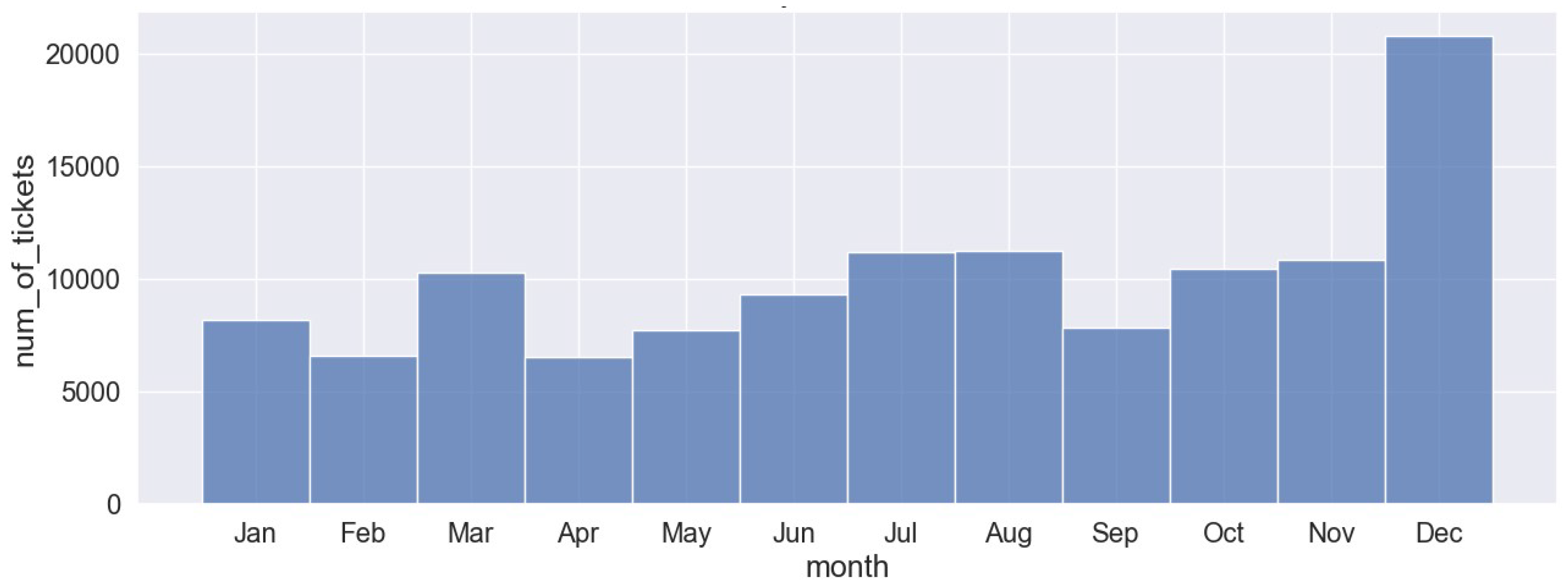
Figure 2.
Ticket sales for Almaty – Astana route in 2022.
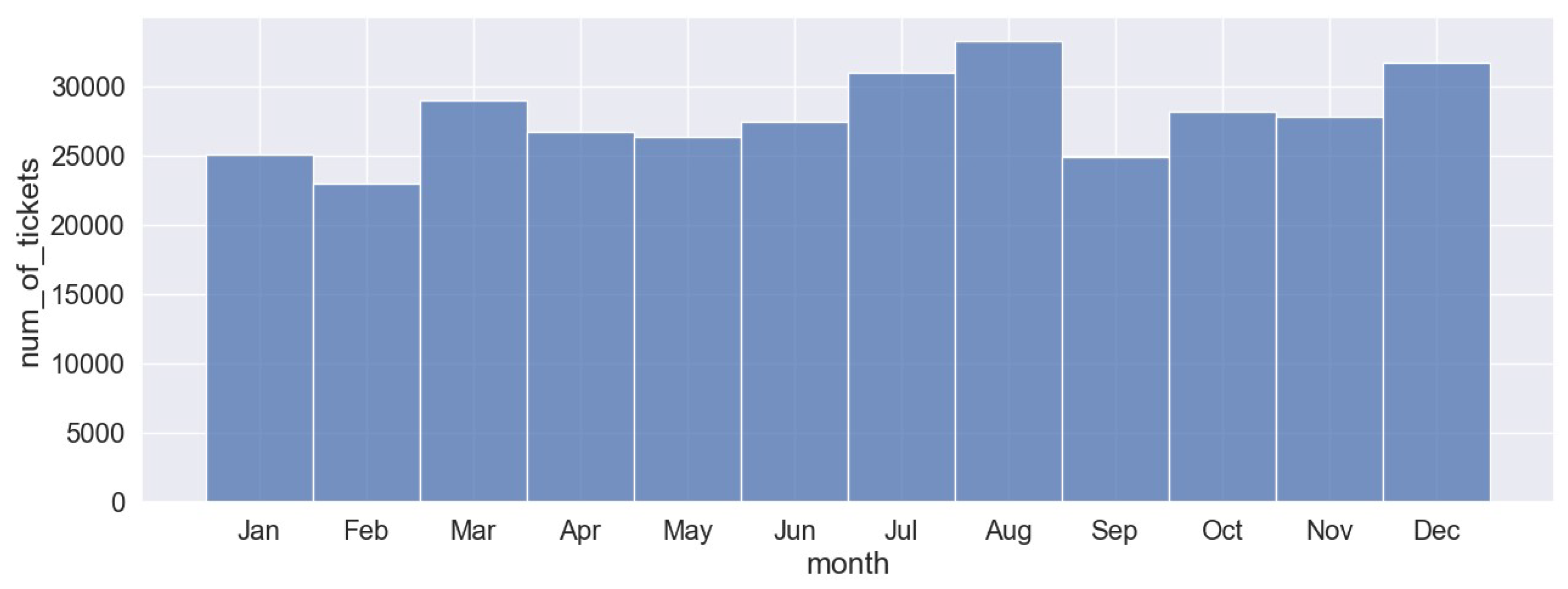
Figure 3.
Ticket sales for Almaty – Astana route in 2023.
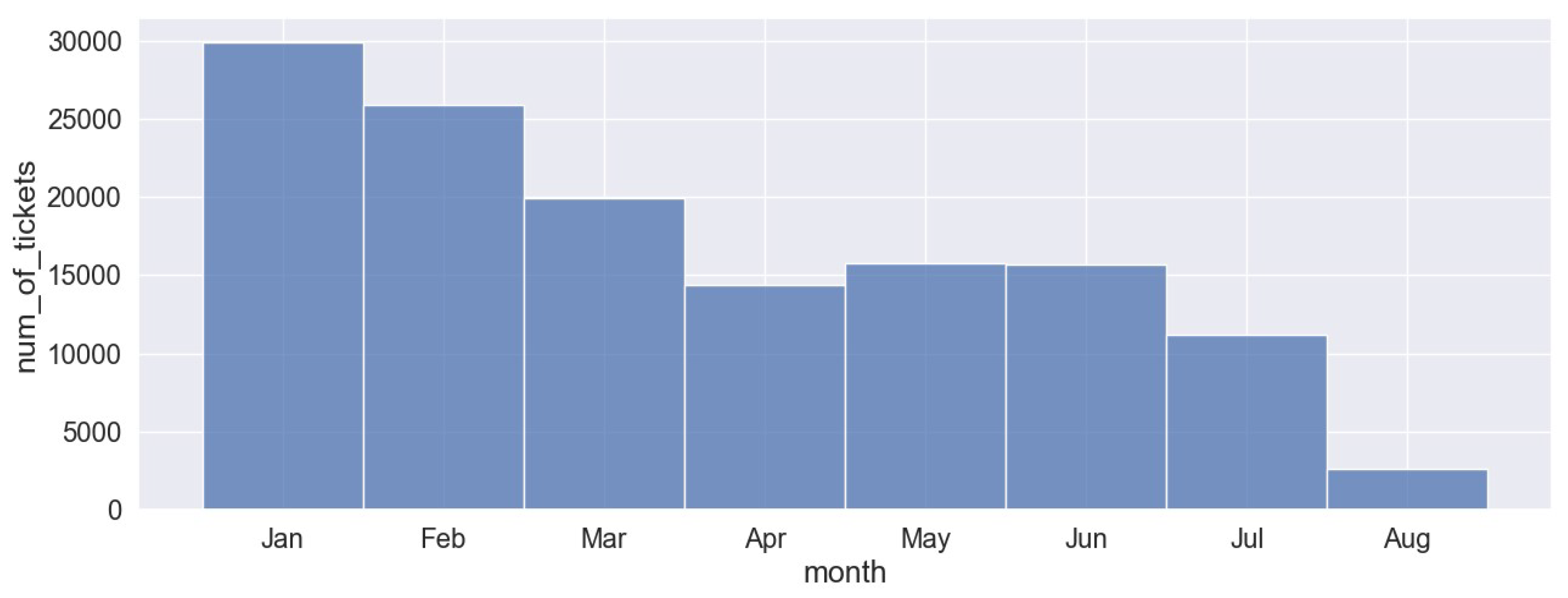
Figure 4.
Ticket sales versus the number of days before departure for Almaty – Astana route in 2021.
Figure 4.
Ticket sales versus the number of days before departure for Almaty – Astana route in 2021.
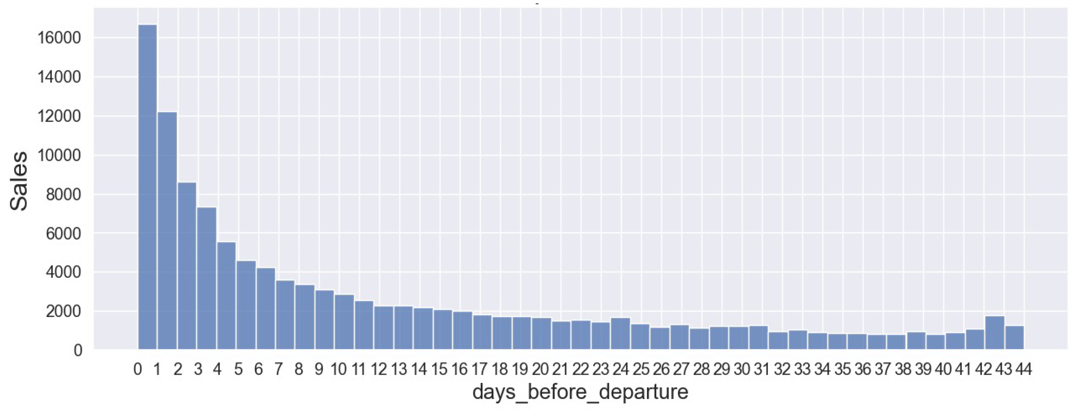
Figure 5.
Ticket sales versus the number of days before departure for Almaty – Astana route in 2022.
Figure 5.
Ticket sales versus the number of days before departure for Almaty – Astana route in 2022.
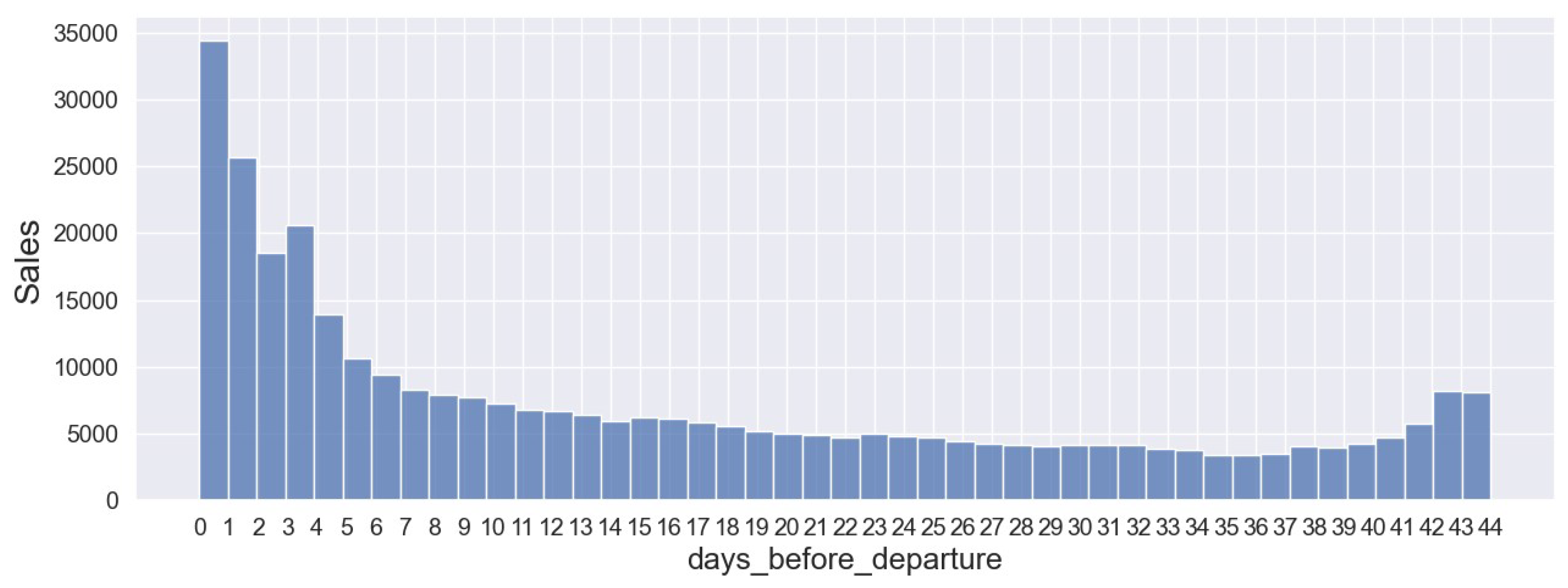
Figure 6.
Ticket sales versus the number of days before departure for Almaty – Astana route in 2023.
Figure 6.
Ticket sales versus the number of days before departure for Almaty – Astana route in 2023.
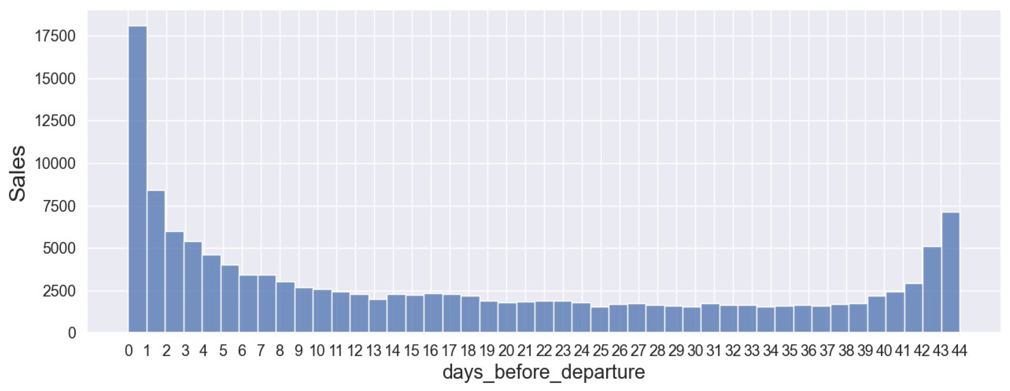
Figure 7.
LSTM model architecture.
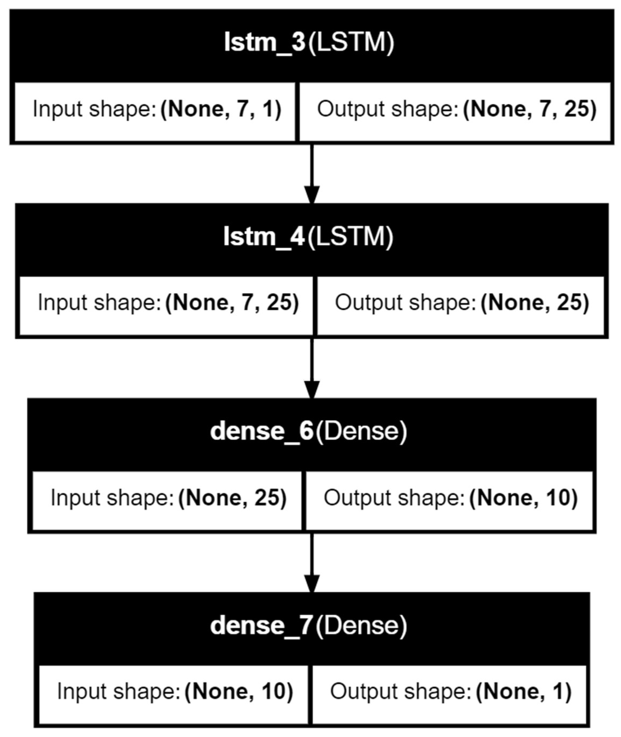
Figure 8.
Schematic representation of OD matrix.
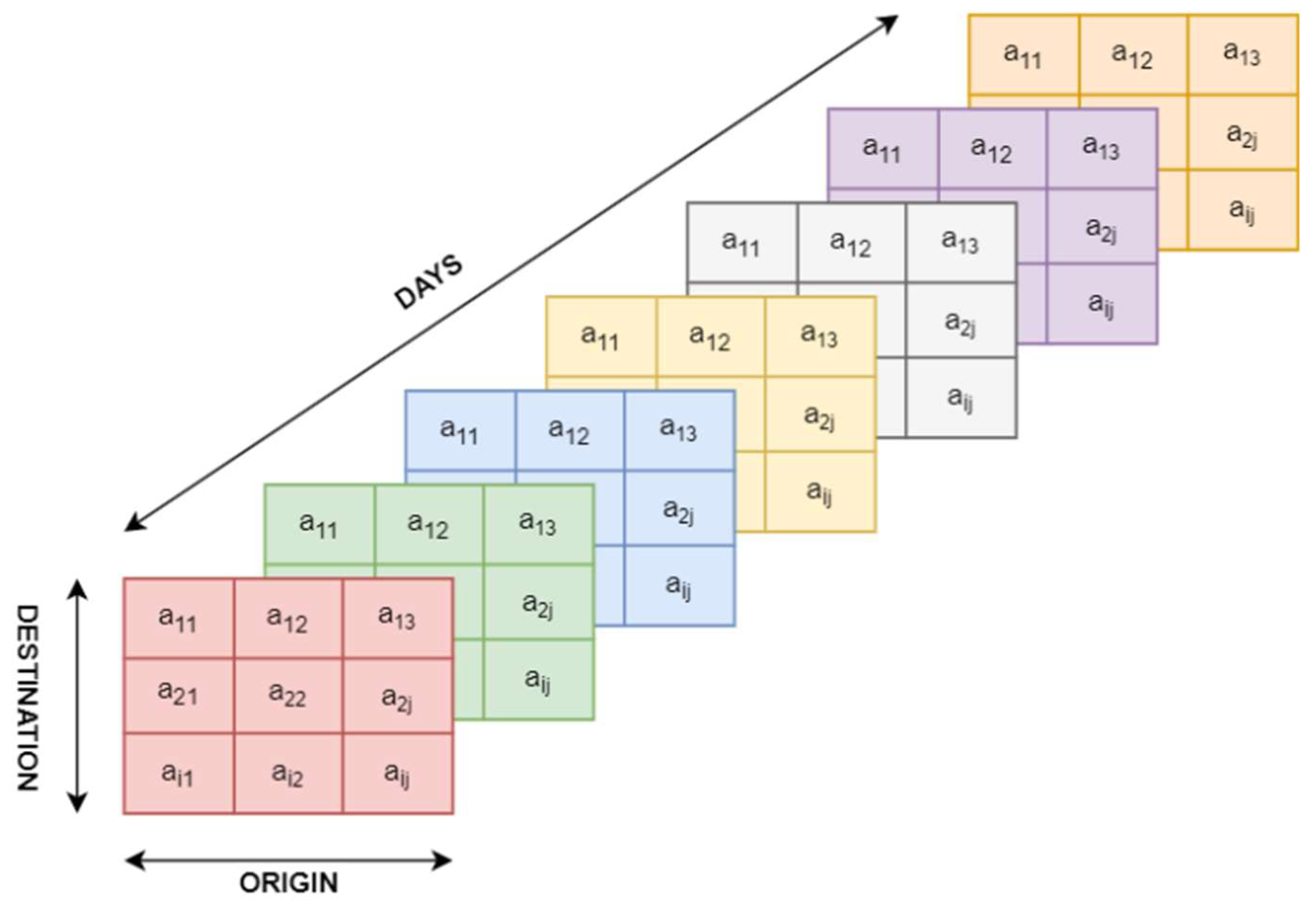
Figure 9.
CNN model architecture.
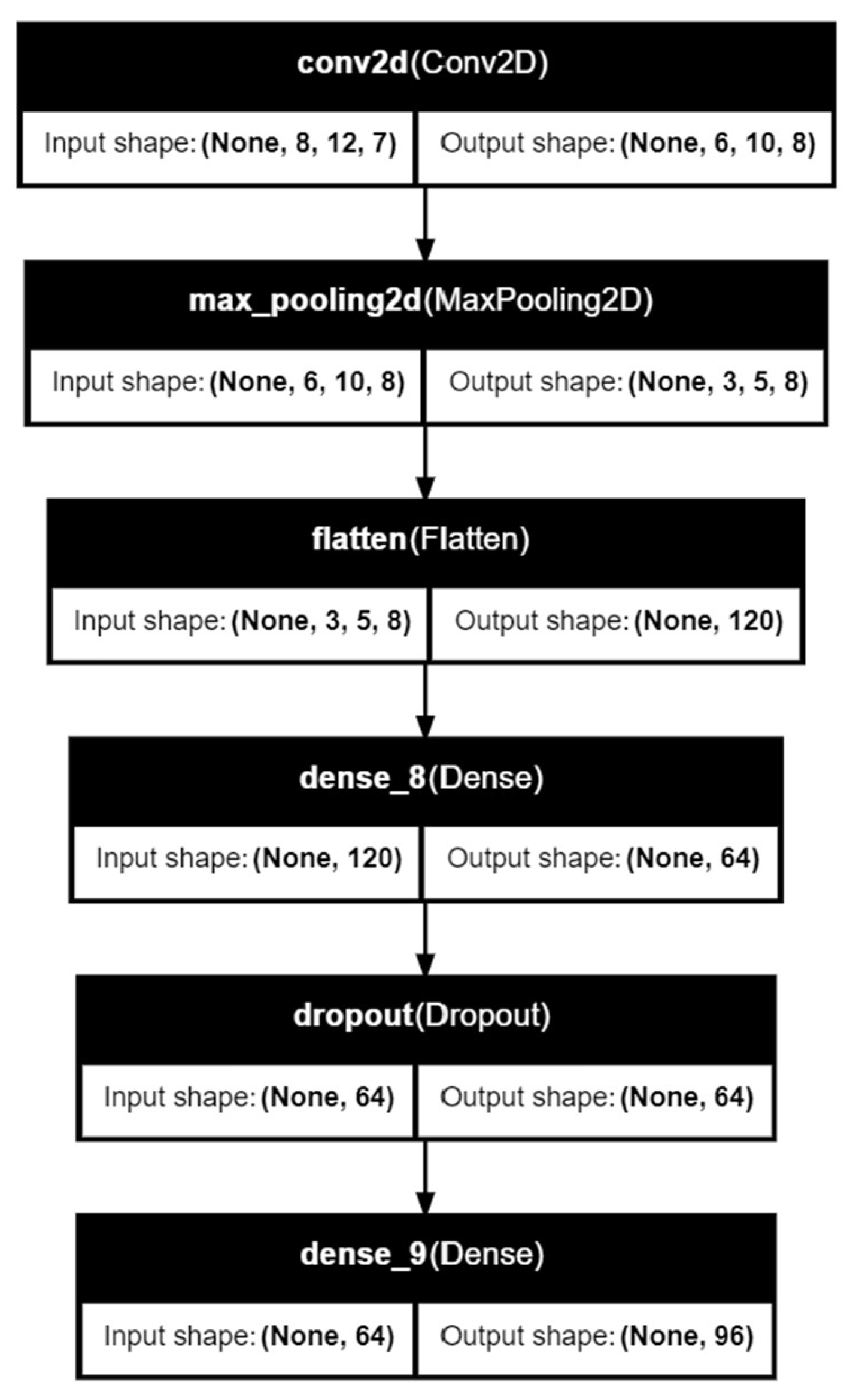
Figure 10.
ARIMA and SARIMAX models’ performance in predicting demand for Almaty – Astana route during November-December 2022.
Figure 10.
ARIMA and SARIMAX models’ performance in predicting demand for Almaty – Astana route during November-December 2022.
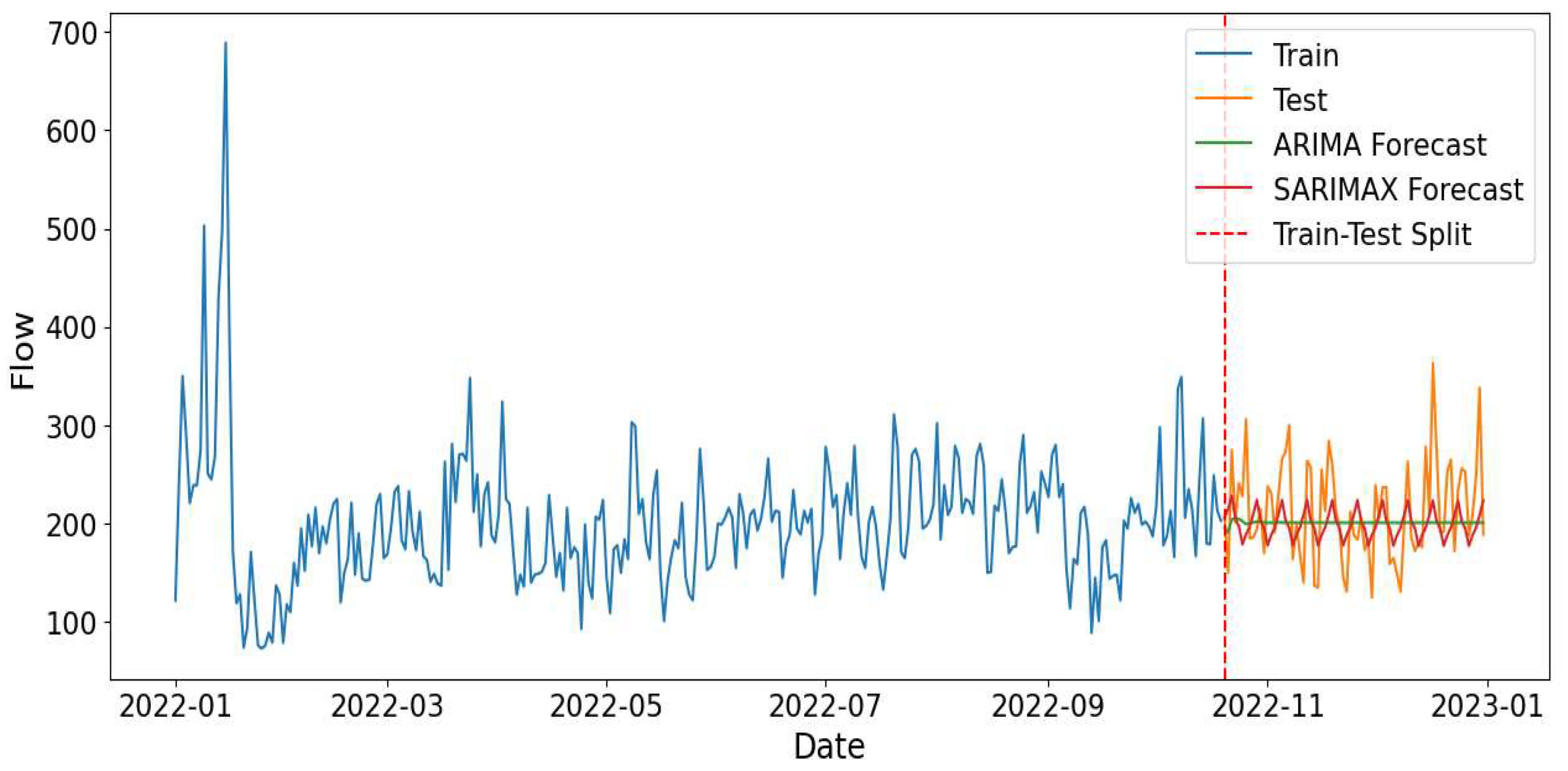
Figure 12.
LSTM model performance in predicting demand for Almaty – Astana route during November-December 2022 .
Figure 12.
LSTM model performance in predicting demand for Almaty – Astana route during November-December 2022 .
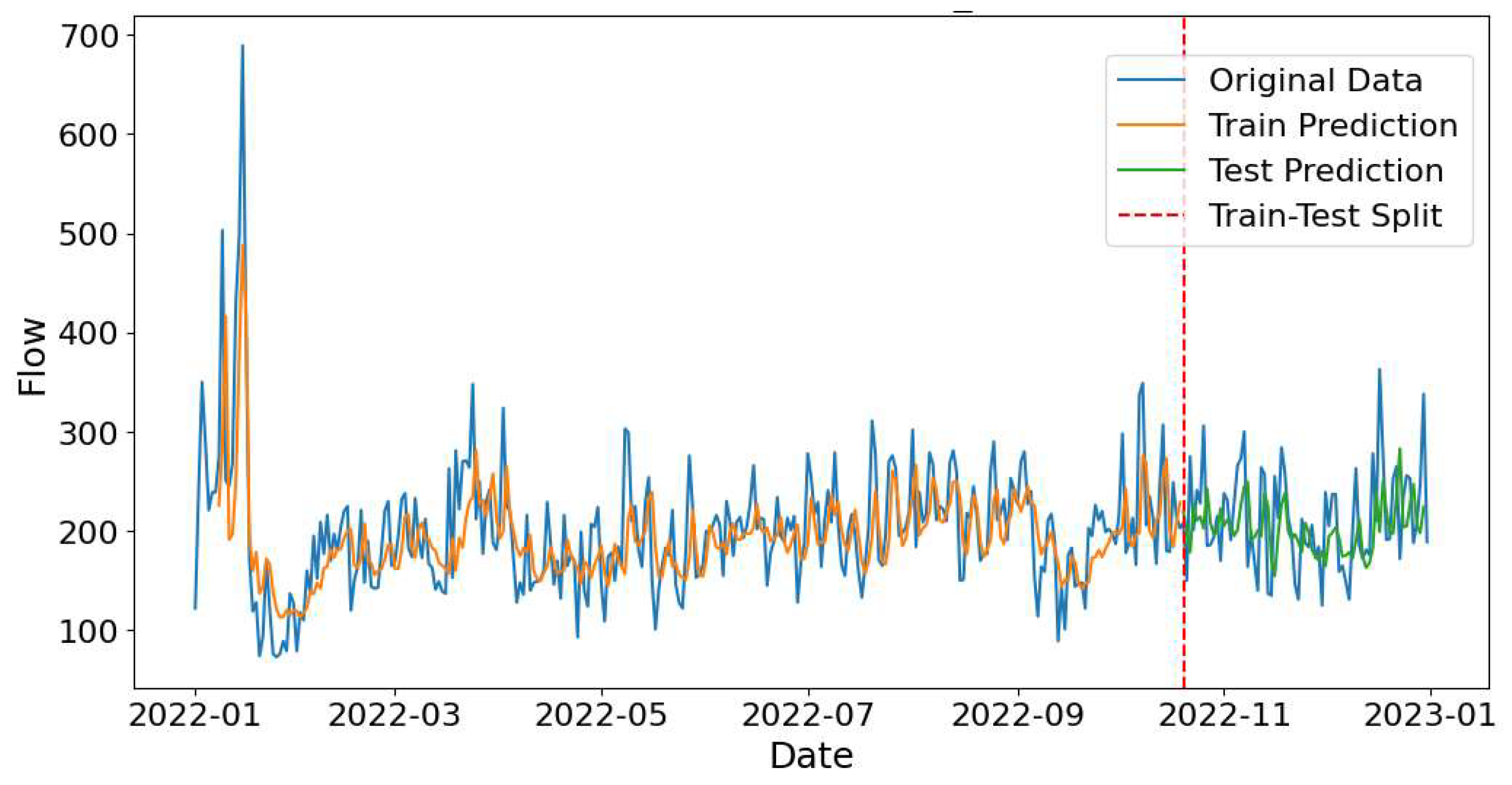
Figure 13.
LSTM model performance in predicting demand for Almaty – Astana route during September 2022 - August 2023.
Figure 13.
LSTM model performance in predicting demand for Almaty – Astana route during September 2022 - August 2023.
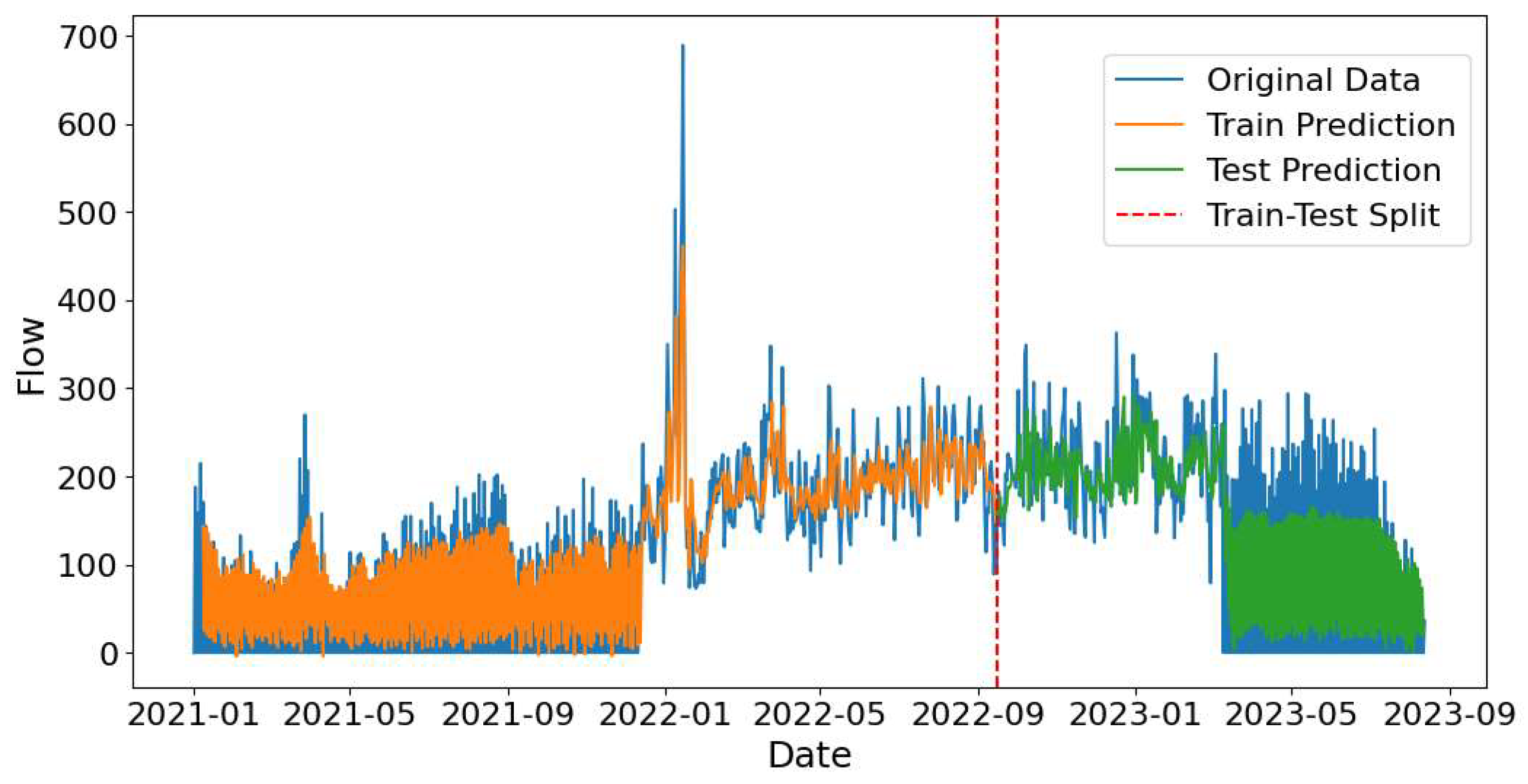
Figure 14.
Training and validation loss curves, LSTM model, test 1.
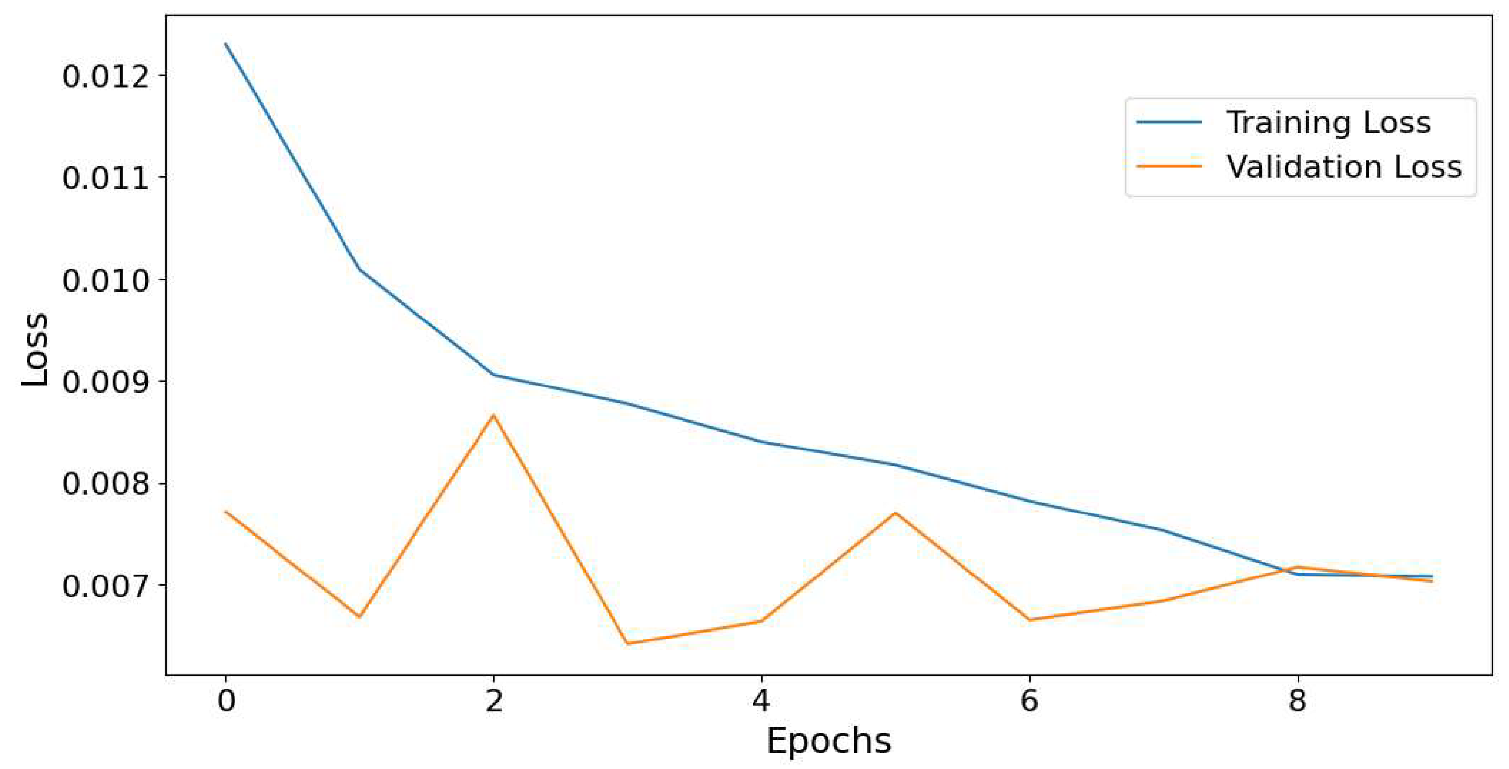
Figure 15.
Training and validation loss curves, LSTM model, test 2.
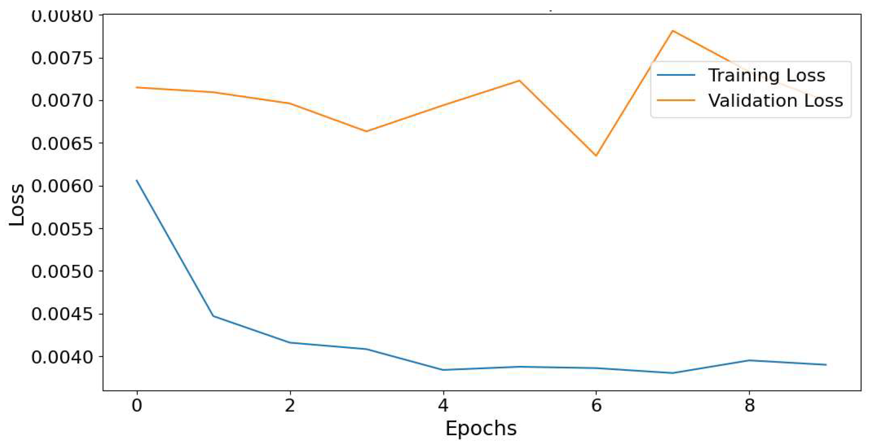
Figure 16.
CNN model performance in predicting demand for Almaty – Astana route during November-December 2022 .
Figure 16.
CNN model performance in predicting demand for Almaty – Astana route during November-December 2022 .
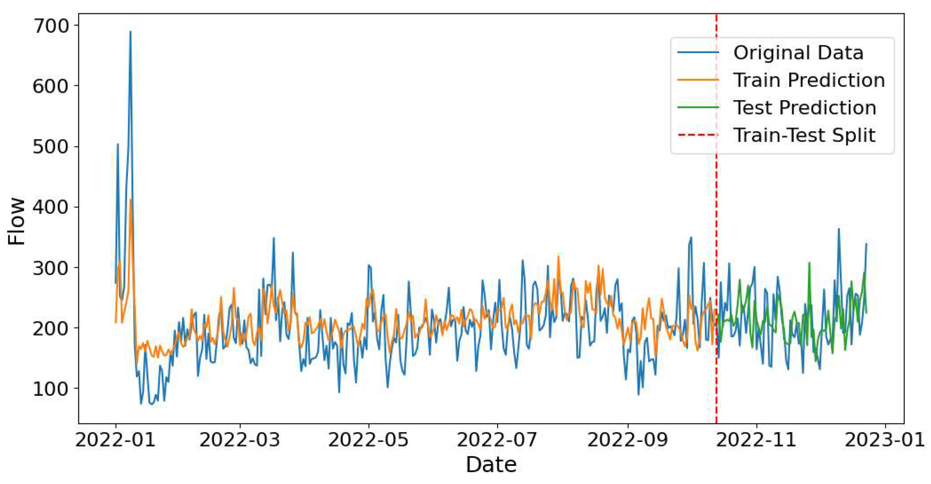
Figure 17.
CNN model performance in predicting demand for Almaty – Astana route during September 2022 - August 2023.
Figure 17.
CNN model performance in predicting demand for Almaty – Astana route during September 2022 - August 2023.
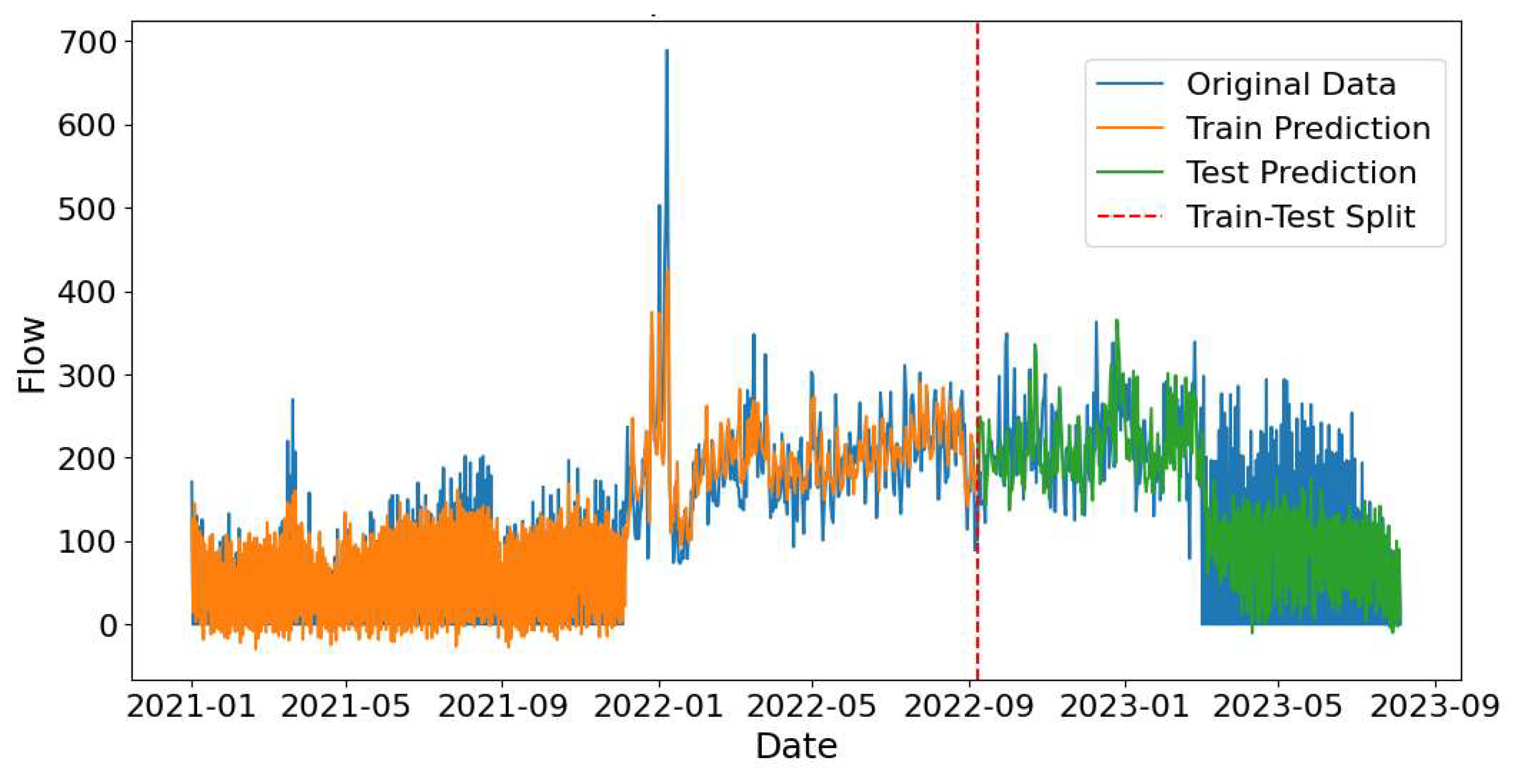
Figure 18.
Training and validation loss curves, CNN model, test 1.
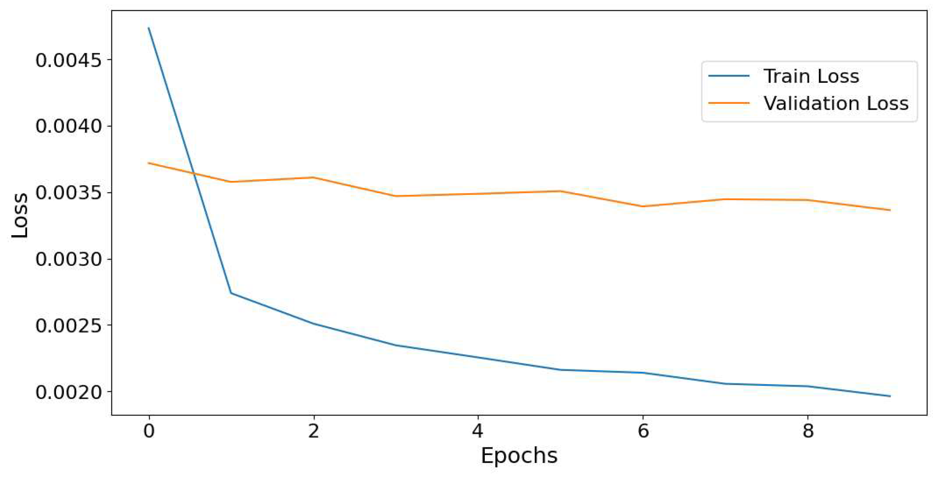
Figure 19.
Training and validation loss curves, CNN model, test 2.
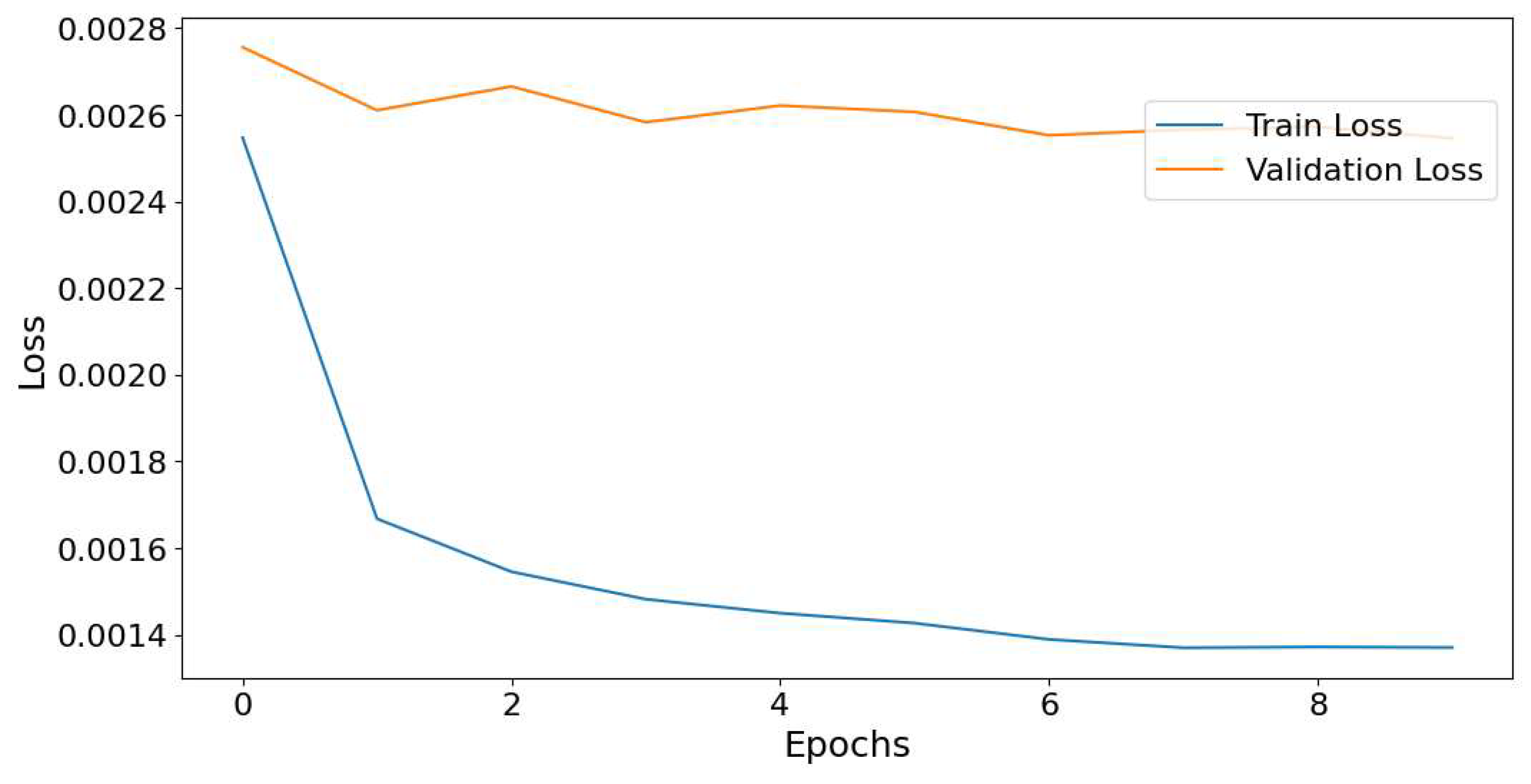
Table 1.
Ticket sales for popular routes from 2021 to 2023.
| OD pair | Number of tickets |
|---|---|
| Almaty – Astana | 127 362 |
| Almaty – Karaganda | 126 906 |
| Astana – Uralsk | 77 795 |
| Astana - Aktobe | 75 514 |
| Aktobe – Uralsk | 29 723 |
| Almaty – Uralsk | 22 600 |
| Karaganda – Astana | 16 675 |
| Astana – Tobol | 14 789 |
| Karaganda – Aktobe | 14 415 |
| Aktobe - Kazakhstan | 14 152 |
Table 2.
ADF test results for first 15 OD pairs.
| OD | p-value | ADF | Status |
|---|---|---|---|
| Almaty – Astana | 2.736E-06 | -5.444 | stationary |
| Almaty – Karaganda | 4.747E-04 | -4.283 | stationary |
| Astana – Uralsk | 0.163 | -1.989 | not stationary |
| Astana - Aktobe | 0.058 | -2.802 | not stationary |
| Aktobe – Uralsk | 0.097 | -2.579 | not stationary |
| Almaty – Uralsk | 0.496 | -1.575 | not stationary |
| Karaganda – Astana | 9.515E-04 | -4.105 | not stationary |
| Astana – Tobol | 0.163 | -2.329 | not stationary |
| Karaganda – Aktobe | 7.961E-07 | -5.694 | stationary |
| Aktobe - Kazakhstan | 0.045 | -2.900 | not stationary |
Disclaimer/Publisher’s Note: The statements, opinions and data contained in all publications are solely those of the individual author(s) and contributor(s) and not of MDPI and/or the editor(s). MDPI and/or the editor(s) disclaim responsibility for any injury to people or property resulting from any ideas, methods, instructions or products referred to in the content. |
© 2024 by the authors. Licensee MDPI, Basel, Switzerland. This article is an open access article distributed under the terms and conditions of the Creative Commons Attribution (CC BY) license (http://creativecommons.org/licenses/by/4.0/).
Copyright: This open access article is published under a Creative Commons CC BY 4.0 license, which permit the free download, distribution, and reuse, provided that the author and preprint are cited in any reuse.


