
Submitted:
31 October 2024
Posted:
01 November 2024
You are already at the latest version
Abstract
We study the Mean-Risk model, where risk is measured by the Modified CoVaR \[ \CoVaR^{\leq}_{\alpha, \beta}(X|Y) = VaR_\beta ( X \;| \; Y + VaR_\alpha (Y) \leq 0).\] We prove that in Gaussian setting, for sufficiently small $\beta$, such model has a solution.
Keywords:
Conditional Value at Risk (CoVaR)
; Porfolio selection
; Gaussian copula
1. Introduction
The question of optimal asset allocation is naturally as old as the history of investing itself, yet the pioneering work of Markowitz is barely over seventy years long and it was as recently as 1990 that the Alfred Nobel Memorial Prize in Economic Sciences was awarded for the theory of portfolio choice (Harry Markowitz), Capital Asset Pricing Model (William Sharpe) and theory of corporate finance (Merton Miller). There are still ample opportunities to explore interesting questions inside that complex field of portfolio analysis. We will pursue the path of investigating conditional value-at-risk, selected instead of variance as the risk measure in the Markowitz model. The task before us is to find the portfolio with the lowest risk while simultaneously retaining the chosen expected return.
To fix the notation, in this paper we will base on the Profit/Loss (P/L) approach as for example in [1,2,7,11,12,20].
We will study random variables X, Y, which are modelling for example: welfare of the financial institutions, financial positions, gains of the investments, or rates of returns of stock prices and indices. So generally
"The higher value of X the better".
The above can be expressed in terms of quantiles. Namely Value-at-Risk at a significance level is equal to minus upper quantile of X or lower quantile of the loss
We recall that for a given random variable X and a given level the set of quantiles is a closed interval , which might be reduced to a point. The end points of the interval are referred to as upper and lower quantiles.
To switch to the alternative Loss/Profit (L/P) approach (applied for example in [3,9,15]) when random variables are modelling losses of the financial investments, actuarial risks or high water levels in hydrology, it is is enough to change the sign of the variables
and remember that, by a convention, the subscript is changed. The significance level is replaced by the confidence level
Now assume, that we are measuring the risk given some stress event. For example, we want to determine how big bailout would be necessary to keep a financial institution X solvent with probability at least when a financial institution Y would perform badly. Conditional Value-at-Risk (CoVaR) introduced in 2008 by Adrian and Brunnermeier ([1]) and its later modifications proved to be very useful tools for measuring (quantifying) such phenomena.
Let X and Y be random variables modelling positions. CoVaR is defined as VaR of X conditioned by Y. In more details:
where a Borel subset of the real line E is modeling some adverse event concerning Y. Most often E consists of one point (a threshold) or is a half-line bounded by a threshold.
As we see, to deal with CoVaR, one has to model the dependence between X and Y. This can be achieved by means of copulas, as can be seen in [2,11,12].
Adrian and Brunnermeier ([1]) applied the construction with E consisting of one point. Such approach has a certain drawback, pointed out for example by Mainik and Schaanning in [15], which is due to the fact that the standard CoVaR is not compatible with the concordance ordering. Hence it is "breaking" the paradigm: more dependence, more systemic risk (see also [11]). To avoid this inconsistency a modified definition of CoVaR was introduced in 2013 and 2014 by Girardi and A.T. Ergün ([8]) and by Mainik and Schaanning ([15]), both in L/P setting.
The modified Conditional-VaR at a level , which is a main objective of this survey, is defined as VaR at level of X under the condition that .
In this survey we consider the portfolio optimization problem with risk measured by the modified CoVaR under the assumption of the normality of returns. It shows that the switch from "standard" CoVaR with one pointed E (see [20]) to modified CoVaR makes the problem more demanding. For example in the "modified" problem, it is not obvious that between portfolios with fixed value and expected value one can find a portfolio minimizing the risk.
The paper is organized in the following way:
In section 2, "Notation", we recall the basics about CoVaR and portfolio selection. In the next one, "The Mean-CoVaR model", we present our main results concerning the existence of optimal portfolios. The following one, "Proofs and auxiliary results", deals with Gaussian copulas and optimization problems. In the last section we provide numerical results concerning a given four-dimensional portfolio.
2. Notation
2.1. CoVaR in the Copula Setting
We present the definition after [2]
Definition .
which can be expressed in terms of quantiles:
We assume that the distribution functions of X and Y are continuous and their joint distribution is described by a copula C.1
From the same article ([2] ) we learn that, since
the following is valid:
Theorem .
where w is the maximal root of the equation:
When furthermore we assume that the pair is normally distributed then
where denotes a Gaussian copula with a parameter (correlation coefficient) and is a distribution function of a univariate standard normal probability law . Thus the impact of Y is encapsulated in the correlation coefficient. The implied significance level w is a function of and .
which is decreasing with .
Furthermore depends on X. For more details see Section 4.1.
2.2. Portfolio Selection
Portfolio (i.e. investment strategy) meets the natural condition of summing up to 1 and is defined as expected value of n-dimensional random variable of returns on risky assets, . Now we add the assumption of normality of R, to be held throughout the rest of the article. To obtain a non-degenerate problem, two more assumptions are made. First, , i.e. not every asset has the same expected return. Second, the covariance matrix of R, is positive definite.
We also define , the univariate random variable of return on the portfolio. Obviously the expected value and the variance are given by
The distribution of X is conditioned on one chosen variable , . Without loss of generality let that be . The correlation coefficient (provided ) is equal to the cosine of the angle between vectors x and in the metric in induced by the scalar product given by the matrix :
where .
We select portfolios with respect to two criteria. We maximize the expected value and minimize the risk measured by CoVaR.
We recall that a portfolio x, , is called efficient, if and only if it is maximal with respect to the generalized Markowitz ordering. Which means that there exists no portfolio y fulfilling the budget constraints , such that
and at least one inequality is strict.
3. The Mean-CoVaR Model
First, we want to find the portfolio x with fixed return which is minimizing CoVaR . The optimization problem presents itself as follows:
where .
The solution of the above problem is closely related to the classical Markowitz problem
We recall that this problem has a unique solution when:
• the symmetric matrix is positively defined i.e. is a matrix of a scalar product on ;
• the vectors and are linearly independent (i.e. not parallel);
•E is any real number.
The solution is given by a formula
where G is a Gram matrix of vectors and with respect to the scalar product defined by the matrix
where by we denote a matrix with columns and . For details see Section 4.2.2.
The existence of the solution of the optimization problem (8) depends on a portfolio , given by a formula:
We recall that , the first coefficient of the vector , is equal to . Note that is orthogonal to vectors and with respect to the standard scalar product and orthogonal to with respect to the scalar product associated to the matrix — for proofs see (52), (). Besides, if we define q in the following way:
then the vanishing of implies that the vectors are linearly dependent.
Theorem .
For linearly independent, the optimization problem (8)
1. has no solution when
2. has a solution when
where is a Gaussian copula with correlation parameter ρ. Moreover, if is a solution of the optimization problem (8), then the vector is parallel to .
where
The proof is provided in Section 4.2.
Remark 3.1.
For solution of the optimization problem (8) may not exist, see Example 5.1.
Next, we want to find the portfolio x which is minimizing CoVaR. The optimization problem presents itself as follows:
where .
Let the vector denotes the derivative of with respect to E. Then
and
Theorem .
For linearly independent, the optimization problem (16)
1. has no solution when
2. has a solutions when
where is a Gaussian copula with the correlation parameter ρ.
The proof is provided in Section 4.2.
Remark .
Note that when the set of the portfolios of the minimal risk is nonempty and bounded then the one with maximal expected value of return is an efficient portfolio. Moreover the existence of the nonempty, bounded set of portfolios of the minimal risk is a necessary and sufficient condition for the existence of the efficient portfolios.
4. Proofs and Auxiliary Results
4.1. Gaussian Copulas
Let us consider a Gaussian Copula:
The correlation coefficient has been added to the copula symbol for the convenience of notation as it is the only other parameter needed for the computation of a copula, due to all elliptical copulas being normalization invariant (c.f. [14], p. 174, Remark 4.3).
Meyer in [17] shows that the Gaussian copula can be extended continuously, approaching the lower and upper Fréchet-Hoeffding bounds, i.e. W and M, respectively; in dimension 2 both of those are copulas.
Following (c.f. [17]) we get an extension of the classical Fréchet-Hoeffding inequality:
Corollary .
Remark .
The Double Gaussian distribution fulfills the following.
For
one has
so that:
Thus
In consequence,
is the strictly increasing function of not only its variables (which is obvious), but also of its parameter . We recall that
Meyer in [17] provides us also with the following formula:
Corollary .
For formula (29) simplifies.
This result is usually attributed to Sheppard [19].
Corollary 4.2 implies:
Corollary 4.3.
Given we have , i.e. :
- (1)
- (2)
- (3)
- .
Remark .
The unique root of the equation
solved for w, with a given , exists for any choice of significance levels , as the horizontal sections of Gaussian copula are continuous, strictly increasing with respect to w:
Moreover, as is strictly increasing with respect to its parameter ρ and is a strictly increasing function of w, we have one-to-one correspondence in the implicit equation.
Remark .
This holds true for and the copula as well. We get (which by the Corollary 4.3. is the minimum value of w). Similarly for and the copula we get .
We denote the above root as .
The following is true:
Note that the equality (30) implies
Moreover is a strictly decreasing, implicit function of and strictly increasing of .
and
4.2. The Optimization Problems
4.2.1. The Basic Problem
We want to find the portfolio x minimizing CoVaR. The optimization problem (8) is equivalent to the following one:
This poses an important question: what if the constraints cannot be satisfied? Now we note only that (being a function of x, ) plays an important role in answering that question. We recall some facts about the cosine when x is moving along a line.
Lemma .
Let
where the nonzero vectors u and w are Σ-orthogonal. Then
and for λ tending to we get
Proof.
Since
we get
The tail expansion follows from the fact that for tending to
□
4.2.2. The Markowitz Problem
As was stated in Section 3 the classical Markowitz problem
has for every , a unique solution when:
• the symmetric matrix is positively defined i.e. is a matrix of a scalar product on ;
• the vectors and are linearly independent (i.e. not parallel).
The solution ( for short) is given by a formula
where G is a Gram matrix of vectors and with respect to the scalar product defined by the matrix
where by we denote a matrix with columns and .
Indeed, fulfills the constraints
Furthermore for any nonzero Y, such that
Since
and
the minimum is attained to . Note that
In the classical approach, where we put
and
we get
It is called the critical line. The variance of the portfolio and the correlation with equal respectively:
Note that is the portfolio of the minimal variance between portfolios fulfilling the constraint . Hence it is -orthogonal to the critical line
Furthermore
For introduced earlier portfolio given by
we obtain
We get also the estimates for the Sharpe ratio
Lemma .
For any portfolio fulfilling the constraint
Proof.
Since both the expected value and standard deviation are homogeneous of degree 1 with respect to the positive multipliers, we may restrict ourself to the case . From the formula (48) we get for portfolios fulfilling the constraints and
Thus
and
Since for portfolios, fulfilling the constraint , formula (48) implies that , we obtain
□
4.2.3. Critical Plane
First we show that the solution of the optimization problem (38) is belongs to the linear plane spanned by two -orthogonal vectors and , which was defined in (12) as:
Note that is orthogonal to vectors and with respect to the standard scalar product and orthogonal to with respect to the scalar product associated to the matrix . Indeed
Furthermore the -scalar product of and is positive, unless . Indeed
Besides, since by (13) we have:
we noted that the vanishing of implies that the vectors are linearly dependent.
4.2.4. Auxiliary Optimization Problem
Now let be a solution of the optimization problem (8) then it solves the following auxiliary problem.
Let be a scalar square of ,
Since is strictly increasing with , is a solution of the optimization problem
Lemma .
The vector
is a unique solution of the optimization problem (57) with .
Proof.
Step 2. Minimum by perturbations.
Let Y be nonzero vector such that
Since and (compare equality (44)),
□
Since is the unique solution of the optimization problem (57) it must be equal to .
4.2.5. Proof of Theorem 3.1
We fix and consider the limiting properties of
when tends to .
Lemma .
where .
Proof.
Since and for a fixed copula C is strictly increasing with w (see Remark 4.2) we have
Note that since we have Lemma 4.1 and is a continuous function,
Therefore for
The last case , , is a bit more complicated. Note that the above assumption implies that
We apply Lemma 4.1 and basing on the formula (37), we obtain
□
Theorem 3.1 is a direct consequence of Lemma 4.4. Indeed:
Point 1. follows from the fact that each member of the family , , is fulfilling the constraints of the optimization problem (38). Since due to lemma 4.4. our target function tends to when , the optimization problem has no solution.
Point 2: Since due to lemma 4.4. our target function tends to when , there exists such that
Hence the minimum is attained to some with .
Furthermore for a solution of the optimization problem (38) the vector is parallel to . □
4.2.6. Proof of Theorem
We start with the following basic case:
Lemma .
Let be a sequence of portfolios fulfilling the constraint , such that:
(i). The variance tends to infinity
(ii). The Sharpe ratio has a limit
(iii). The correlation coefficient with has a limit
Then
Proof.
We observe that
Since
we get for
□
If we add to assumptions from the above lemma, the additional assumption that the sequence belongs to the critical half-plane, than we get the dependence between the limiting values and .
Lemma .
Let
Then the assumptions from Lemma 4.5 imply that:
and
Proof.
From the definition of the Sharpe ratio we get
Thus
This implies that the ratio has a limit. Basing on the formula (48) we get
Obviously the above implies that
Next
□
In order to prove point 1 of Theorem we provide for any such that
a sequence such that
We put
We get
and
Hence, due to Lemma 4.6
Finally Lemma 4.5 implies that the limit from (74) equals .
Next we prove point 2 of Theorem . We assume that
We denote by the infimum of the CoVaR,
Let the sequence be a sequence of portfolios approaching ,
We show that the assumption (78) implies that the sequence must be bounded. Indeed, otherwise there would exist a subsequence such that
Since the Sharpe ratios
and correlation coefficients
belong to a bounded sets (see Lemma 4.2) we might select the subsequence in such a way that these ratios and coefficients have limits. We denote these limits by and
Due to Lemma 4.3 (, ) and Lemma 4.6
Thus the assumption (78) and Lemma 4.5 imply that
which contradicts the assumption that the sequence is approaching the infimum of CoVaR.
5. Examples
We consider the following data:
We get
Finally
We fix E and study the halfline of portfolios
Example .
We have . We choose
This way we get
Therefore
where
for any and in consequence . From Lemma 4.4., we have that:
Thus the global minimum cannot exist. We illustrate this at Figure 3.
Example .
We consider the same data. However, now we choose
This way we get and the optimization problem has a solution. We have
where .
For we have . We get numerically calculated minimum for as illustrated at Figure 4.
For we have . We get numerically calculated minimum for as illustrated at Figure 5. As the reader can guess, it has been easier to subtract a certain constant from CoVaR to show how the new function is positive for .
For we have . We get numerically calculated minimum for as illustrated at Figure 6.
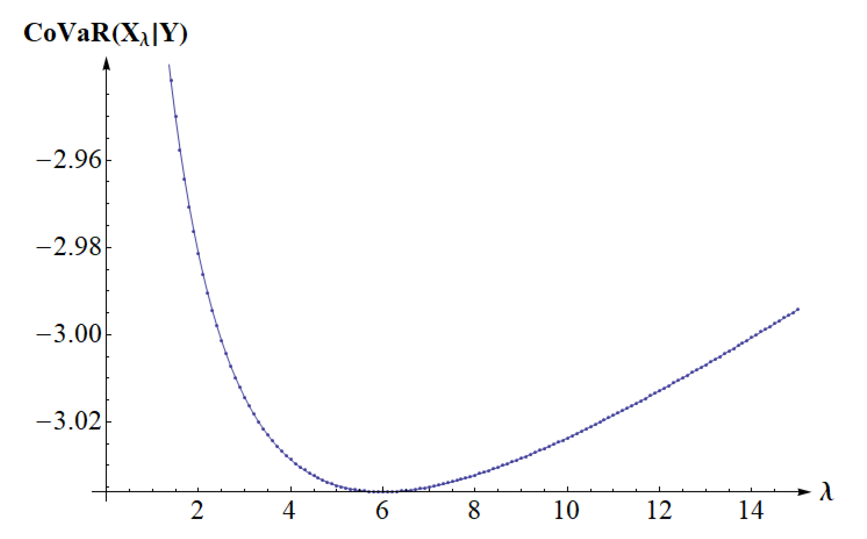
For we get . We get numerically calculated minimum for as illustrated at Figure 7.
All the numerical calculations seem to point to the existence of unique solution under condition from Theorem .
References
- Adrian, T., Brunnermeier, M.K.: CoVaR, The American Economic Review 106.7, 1705-1741 (2016).
- Bernardi, M., Durante, F., Jaworski, P., 2017. Covar of families of copulas. Statistics & Probability Letters 120, 8–17.
- Bernardi, M., Durante, F., Jaworski, P., Petrella, L., Salvadori, G.: Conditional Risk based on multivariate Hazard Scenarios. Stochastic Environmental Research and Risk Assessment 32 (2018) 203-211.
- Cherubini, U., Luciano, E., Vecchiato, W.: Copula Methods in Finance, John Wiley & Sons Ltd 2004.
- Durante, F., Sempi, C.: Principles of copula theory, CRC Press 2016.
- Embrechts, P.: Copulas: a personal view. Journal of Risk and Insurance, 76, 639–650 (2009).
- Föllmer, H., Schied, A.: Stochastic Finance. An Introduction in Discrete Time, de Gruyter, 2nd Edition, 2004.
- Girardi, G., Ergün T.A.: Systemic risk measurement: Multivariate GARCH estimation of CoVar, Journal of Banking & Finance 37, (2013) 3169-3180.
- Hakwa B., Jäger-Ambrozewicz, M., Rüdiger, B.: Analysing systemic risk contribution using a closed formula for conditional Value at Risk through copula. Commun. Stoch. Anal., 9(1):131–158, 2015.
- Jaworski, P.: The limiting properties of copulas under univariate conditioning, In: Copulae in Mathematical and Quantitative Finance, P.Jaworski, F.Durante, W.K.Härdle (Eds.), Springer 2013, pp.129–163.
- Jaworski, P., On the Conditional Value at Risk (CoVaR) for tail-dependent copulas, Dependence Modeling 5 (2017) 1-15.
- Jaworski, P., On the Conditional Value-at-Risk (CoVaR) in copula setting, W: Úbeda Flores, M., de Amo Artero, E., Durante, F., Fernández-Sánchez, J. (Eds.) Copulas and Dependence Models with Applications, Springer, Cham 2017, pp. 95-117.
- Joe, H.: Dependence Modeling with Copulas. Chapman & Hall/CRC, London, 2014.
- Mai, J., Scherer, M., 2012. Simulating Copulas: Stochastic Models, Sampling Algorithms, and Applications. Series in quantitative finance. Imperial College Press.
- Mainik G., Schaanning E.: On dependence consistency of CoVaR and some other systemic risk measures. Stat. Risk Model., 31, 49–77 (2014).
- McNeil, A.J., Frey, R., Embrechts, P.. Quantitative risk management. concepts, techniques and tools. Princeton Series in Finance. Princeton University Press, Princeton, NJ, 2005.
- Meyer, C., 2013. The bivariate normal copula. Communications in Statistics - Theory and Methods 42 (13), 2402–2422.
- Nelsen, R.B.: An introduction to copulas. Springer Series in Statistics. Springer, New York, second edition, 2006.
- Sheppard, W.F., 1900 On the calculation of the double integral expressing normal correlation. Trans. Camb. Phil. Soc., 19, 23-68.
- Zalewska, A., 2018. On peculiarities of covar-based portfolio selection. Applicationes Mathematicae, 181–197.
| 1 |
Figure 1.
Horizontal sections of a chosen Gaussian copula
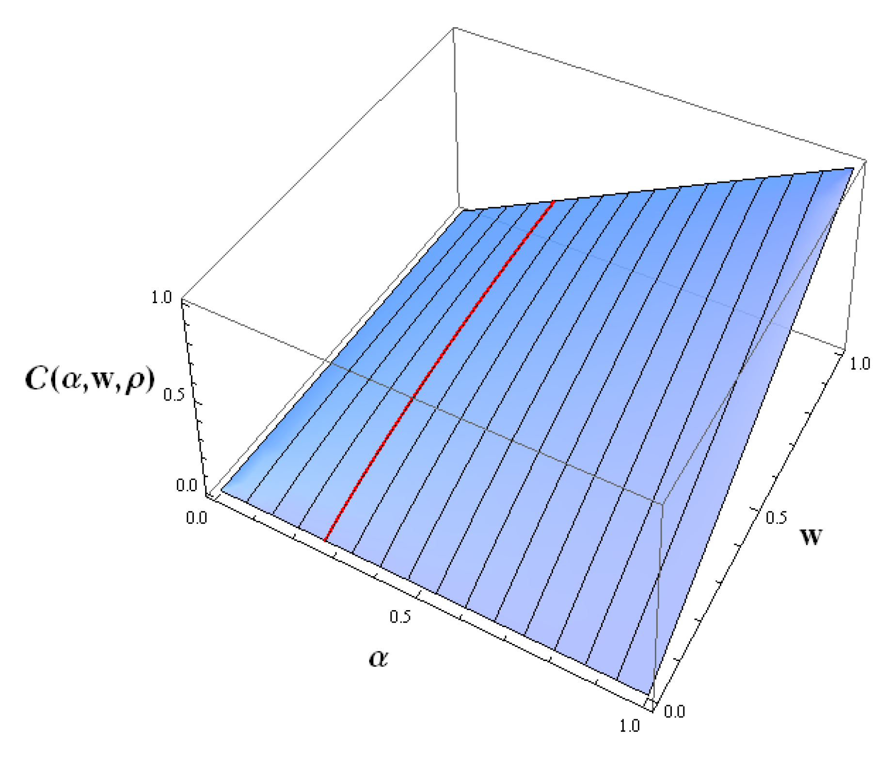
Figure 2.
Graph of the function .
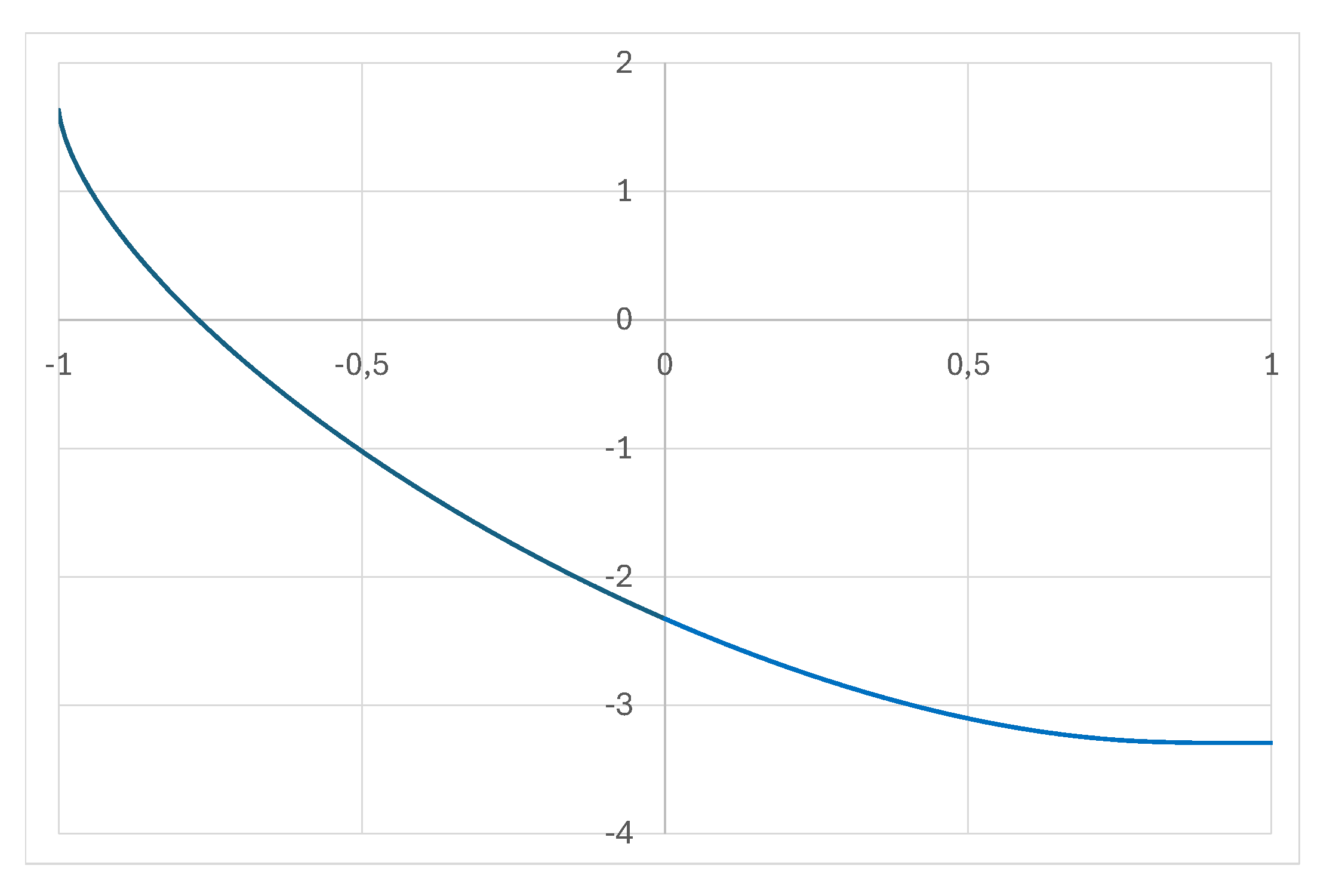
Figure 3.
Numerically calculated CoVaR as the function of
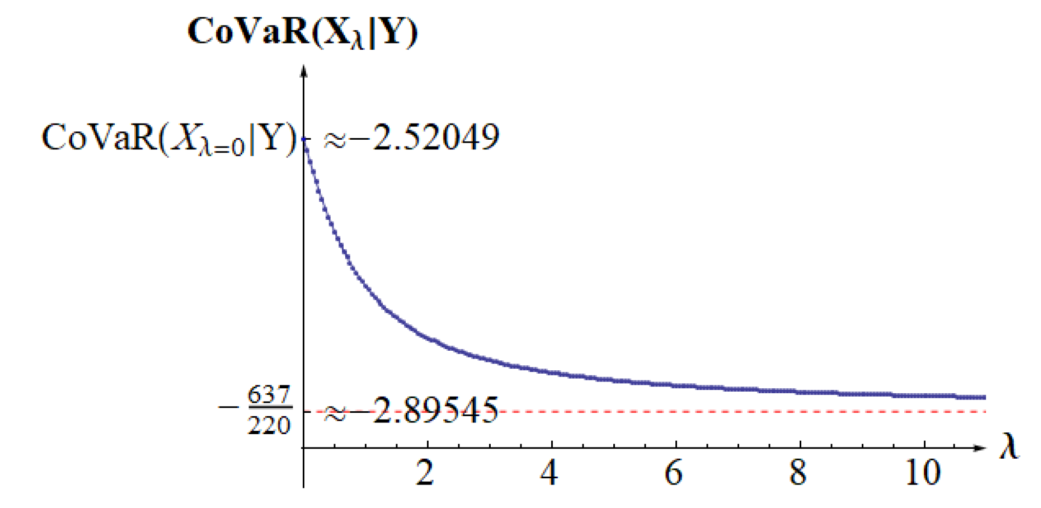
Figure 4.
Numerically calculated CoVaR for
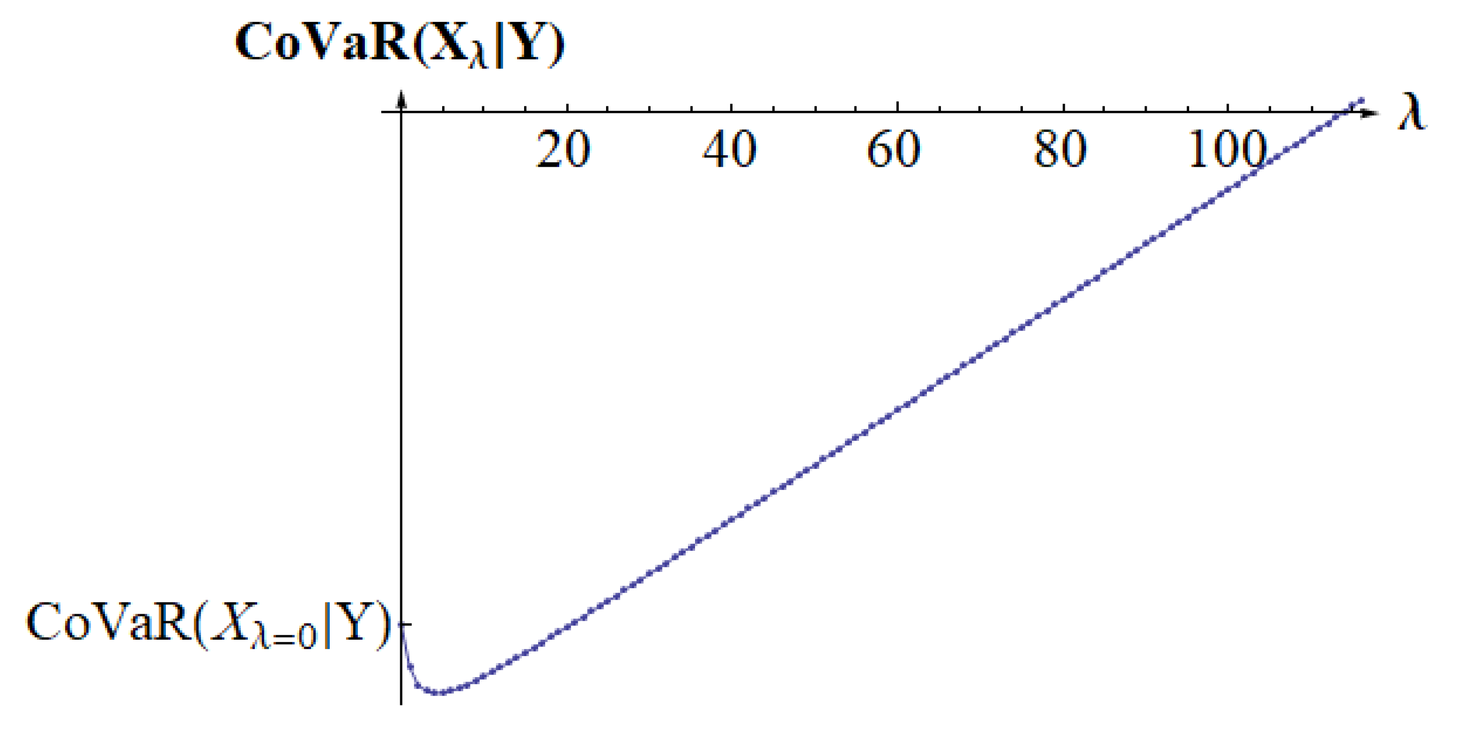
Figure 5.
Numerically calculated for
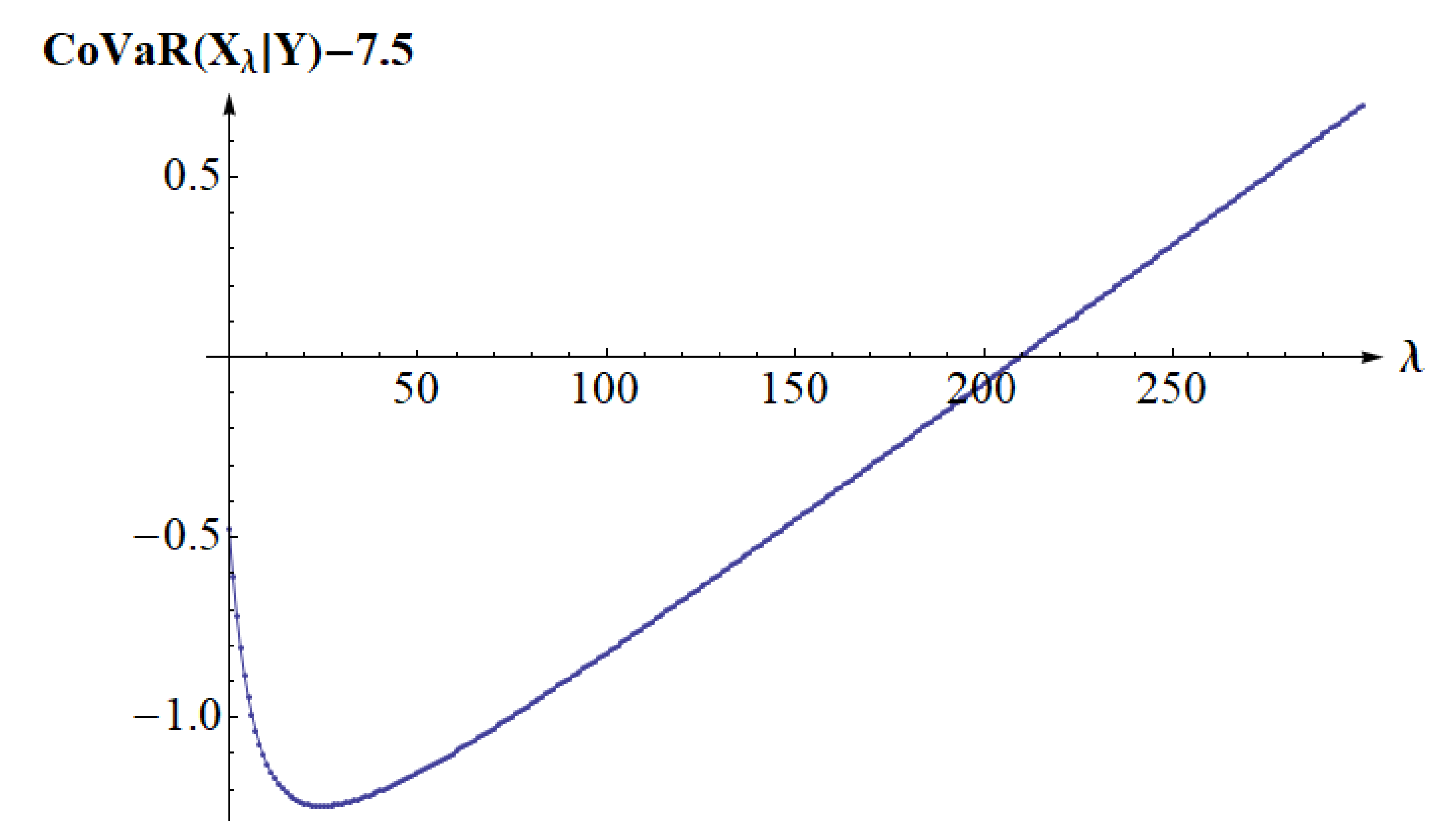
Figure 6.
Numerically calculated CoVaR for
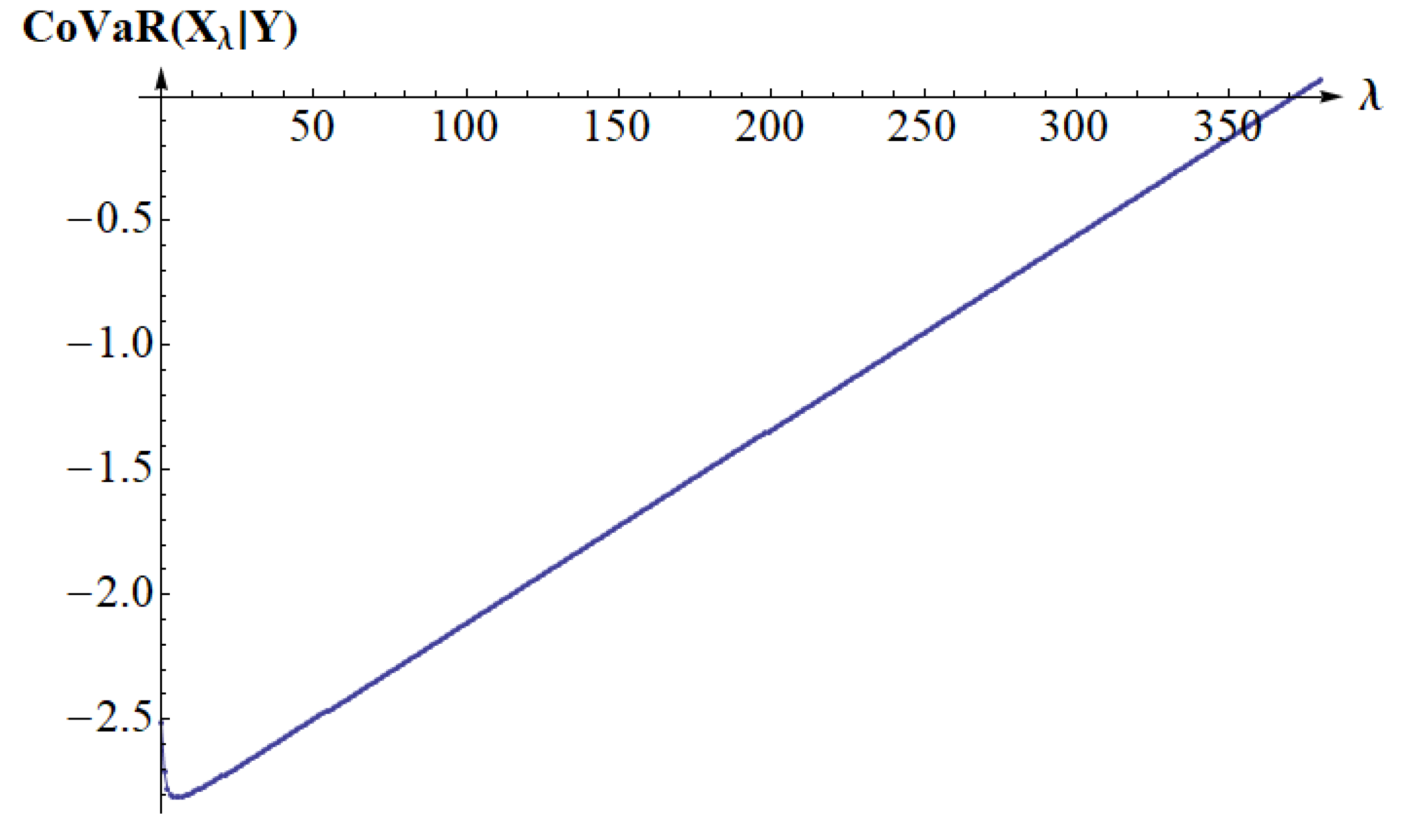
Figure 7.
Numerically calculated CoVaR for
Disclaimer/Publisher’s Note: The statements, opinions and data contained in all publications are solely those of the individual author(s) and contributor(s) and not of MDPI and/or the editor(s). MDPI and/or the editor(s) disclaim responsibility for any injury to people or property resulting from any ideas, methods, instructions or products referred to in the content. |
© 2024 by the authors. Licensee MDPI, Basel, Switzerland. This article is an open access article distributed under the terms and conditions of the Creative Commons Attribution (CC BY) license (http://creativecommons.org/licenses/by/4.0/).
Copyright: This open access article is published under a Creative Commons CC BY 4.0 license, which permit the free download, distribution, and reuse, provided that the author and preprint are cited in any reuse.


