
Submitted:
29 October 2024
Posted:
30 October 2024
You are already at the latest version
Abstract
The application of deep learning convolutional neural networks (CNNs) for rock image characterization has become a prominent method in petroleum geology both nationally and internationally. Precise and automated segmentation of rock sheet images is essential for effective analytical studies. This research addresses the limitations of traditional image segmentation methods, which suffer from low accuracy and high costs in analyzing reservoir rock flakes. We propose an advanced model based on the U-Net architecture, incorporating both attention mechanisms and residual networks. The inclusion of residual modules enhances the network's depth, while the Convolutional Block Attention Module (CBAM) improves feature representation by adjusting the weighting of learned information. Extensive experimental results demonstrate that this approach delivers superior segmentation performance, marking a significant advancement in the field of reservoir rock image analysis.
Keywords:
ResUNet-CBAM model
; attention mechanism
; image segmentation
; deep learning
; rock thin section image
1. Introduction
Grain size analysis of rock particles using thin section images is a common method in geological laboratories, and the segmentation of rock thin sections is a prerequisite for particle size analysis and mineral identification [1]. Pores in rock thin sections serve as essential pathways for fluid presence within rocks[2]. The unique pore and fracture structures in reservoir rocks enable the storage and migration of hydrocarbons[3]. Precise analysis of pore structure can enhance oil recovery rates, support reservoir evaluation, and aid in hydrocarbon production forecasting. Thin section image segmentation is typically the first step in processing rock thin section images, helping geological researchers to more clearly present pores, minerals, and other targeted features. However, current thin section image segmentation faces challenges, such as multiple target similarity, sample variability, and equipment inconsistency. Traditionally, rock segmentation tasks have been conducted by professionals relying on personal expertise. However, this approach is labor-intensive, and segmentation results are subject to subjective influences, lacking consistency and stability[4].
In traditional image segmentation algorithms, images often lack global semantic information, leading to poor generalization and an inability to handle complex and variable scenarios effectively. Previous methods for segmenting rock casting images mainly relied on traditional color-space-based segmentation of pore regions[5]. Zhang Ting et al. employed a morphological watershed algorithm to detect pore edges, achieving continuous and closed pore edge information; however, this method is highly sensitive to noise and variations in grayscale values[6]. Region-based seed point growth methods have also been used to segment particles and pores in rock thin section images[7]. B. Obara segmented images within different color spaces based on the specific characteristics of various rock images[8]. Gorsevski marked boundary pixels in rock images and used these boundary pixels as segmentation guides, but this approach often produced false edges, resulting in inaccurate segmentation[9].
With the advancement of deep learning in image processing, traditional segmentation methods have fallen behind in terms of speed and accuracy compared to deep learning techniques. The development of encoder-decoder base models, fully convolutional networks[10], and atrous spatial pyramid pooling[11] has significantly enhanced the resolution of segmented output images. Common encoder-decoder models include U-Net, proposed by Ronneberger et al.[12], and U2-Net, developed by the University of Alberta in 2020[13]. U2-Net features an RSU (Residual U-block) structure, where each RSU is a miniature U-Net, and the final model is constructed through skip connections in an FPN (Feature Pyramid Network). These networks have achieved notable success in fields such as medicine and remote sensing. For example, He Junyi et al.[14] utilized an improved U-Net network to segment pores and fractures in concrete CT images, effectively enhancing segmentation accuracy. Liang Yan et al.[15] used an encoder-decoder structure in UNet3+ to detect changes in buildings from remote sensing images. In the field of rock analysis, several researchers have also applied convolutional neural networks to process rock images. For instance, Liu Yong et al.[16] proposed an improved SKNet and Bi-GRU for mineral identification in thin-section images, while Dong Ling et al.[17] developed an edge segmentation algorithm for core particle images based on an improved SLIC method.
Although deep learning methods outperform traditional techniques to some extent, they also present certain issues. For instance, Li Zhou et al. used the deep learning segmentation network FCN to extract pores in casting images, but due to information loss during the pooling stages in FCN, the extraction results were suboptimal, and the model’s practical applicability was limited by external factors[18]. Cai Yuheng et al. proposed a model based on a UNet backbone, incorporating residual blocks and atrous convolutions in the encoder to enhance the network’s depth and width. However, in the decoder, they only used simple short links for feature fusion, which led to poor segmentation performance on lower-resolution casting thin sections, indicating limited generalization ability[19]. Additionally, current segmentation methods for particles are prone to interference from complex backgrounds, and the mutual adhesion between particles often results in inaccurate segmentation.
To address the issues mentioned above, this paper proposes an optimized improvement based on the UNet architecture. In the encoding phase at the input stage, residual structures are employed to further increase the network depth and extract deeper semantic features. In the decoding phase, the CBAM attention mechanism is used to suppress the learning weights of irrelevant regions and calibrate the convolved images, thereby achieving ideal segmentation results. Specifically, the CBAM module combines channel attention and spatial attention to selectively enhance features along these two dimensions. CBAM first extracts global information through global average pooling and global max pooling, then uses this information to generate weights for each channel and spatial location. These weights reinforce important features and suppress irrelevant or noisy information, achieving effective feature selection. Experimental results demonstrate that this approach exhibits superior segmentation performance and generalization ability in rock thin-section image segmentation tasks.
2. Related Technologies
2.1. Basic U-Net Network Model
U-Net, proposed by Ronneberger et al. in 2015, is a U-shaped symmetric network structure primarily composed of an encoder-decoder (Encoder-Decoder) architecture, as shown in Figure 1[12]. The encoder is mainly responsible for downsampling the image. It performs four rounds of downsampling, where each level applies two 3×3 convolutional layers followed by a 2×2 max pooling layer with a ReLU activation function. After two 3×3 convolutions at each level, a 2×2 max pooling operation is applied, reducing the feature map size while doubling the number of filters, thereby capturing and propagating semantic information and completing the extraction of feature pixels.The decoder, on the other hand, is responsible for upsampling the feature maps. It performs four rounds of upsampling using 2×2 transposed convolution layers and skip connections between the encoder and decoder. During each upsampling step, information from the corresponding downsampling layers and the input of the upsampling layer itself is integrated, expanding the feature map dimensions while halving the number of filters. This process gradually restores the pixel information and resolution of the segmented feature map.
2.2. Residual Network ResNet
Before the introduction of ResNet, it was generally believed that network depth was positively correlated with model performance—that is, the deeper the network, the stronger its capability to extract high-level semantic information. However, experimental results showed that simply building a deep network in the same manner as a shallow network could lead to a decrease in model performance. This is because, as network depth increases, training difficulty rises significantly, making it ineffective to improve deep networks merely by adding more layers. Residual Networks (ResNet), proposed by He et al. in 2016, introduced skip connections to address this issue, making it a breakthrough in neural network design [20]. A residual network consists of the upper-layer output X and the network mapping F(X) before summation. The mapping H(X) represents the network mapping after the summation. Compared to conventional deep neural networks, where the goal is to learn a direct mapping from X to H(X) (as shown in Figure 2(a)), the introduction of residuals transforms this process. Instead of directly mapping X to H(X), the residual approach aims to find the mapping H(X) = X + F(X), where F(X) = H(X) - X, making it a residual function. If F(X) = 0, then an identity mapping H(X) = X is achieved, as illustrated in Figure 2(b). This approach simplifies the mapping process, reducing the parameters that need to be calculated within the module, and enhances sensitivity to changes by highlighting subtle differences after removing the main component X.In this task, the input X should contain as much clear and complete information from the rock thin-section images as possible, particularly emphasizing areas that display key features like grains and pores. For maximal activation, the input X should be high-resolution, with well-balanced color and contrast, allowing the network to extract prominent features across different layers effectively.
The specific implementation involves replacing the encoder part of U-Net with ResNet’s pre-trained model, which includes 50 layers of residual blocks. The pooling and upsampling operations in U-Net are removed, retaining ResNet’s convolutional layers and residual blocks. Skip connections are added between each residual block to transfer more low-level feature information to the decoder. The decoder part is then added above the final layers of ResNet, including upsampling operations and convolutional layers, to restore the feature map’s dimensions and detail information. This approach leverages ResNet’s powerful feature extraction capability to replace the encoder in the original U-Net model, thereby enhancing the mode’s performance and representational capacity. The specific fusion structure is illustrated in Figure 3.
2.3. CBAM Module
In recent years, with the rapid development of deep learning in the field of computer vision, attention mechanisms have been widely applied in research areas such as image classification, semantic segmentation, and natural language processing. Convolution operations, as the most frequently used module in convolutional neural networks, operate by blending features within the local receptive field across spatial and channel dimensions, thereby capturing multi-dimensional, multi-scale spatial information. However, for different image classification tasks, the importance of information across different channels and spatial locations varies. Simply merging all channel and spatial information without differentiation can result in the loss of important details. To address this, Woo et al. introduced the Convolutional Block Attention Module (CBAM) in 2018[21]. CBAM combines channel and spatial attention mechanisms, establishing relationships among channels while learning weights for spatial positions. This module enhances the learning weights for essential information while suppressing irrelevant information that has minimal impact on network performance, thus improving the feature representation capability of convolutional neural networks, as shown in Figure 4.
The Convolutional Block Attention Module (CBAM) is a lightweight and effective attention mechanism that enhances feature representation by focusing on both channel and spatial information. CBAM consists of two sub-modules: the Channel Attention Module and the Spatial Attention Module.
1. Channel Attention Module: First, the CBAM module takes an input feature map X with dimensions RH×W×C, where H and W represent the height and width of the feature map, and C denotes the number of channels. In the Channel Attention Module, global information is extracted through global average pooling and global max pooling operations, each generating a feature vector with dimensions R1×1 ×C. These two vectors are processed through a shared Multi-Layer Perceptron (MLP), which consists of a fully connected layer (reducing the dimension to C/r, where r is the reduction ratio), followed by a ReLU activation function, and then another fully connected layer (restoring the dimension to C). The two outputs are summed and passed through a Sigmoid activation function to generate channel attention weights. Finally, these weights are multiplied, channel-wise, with the original feature map to highlight significant feature channels and suppress irrelevant channel information. The structure is shown in Figure 5.
The output MC(F) of the Channel Attention Module can be calculated using the following formula:
where F is the input feature map, AvgPool and MaxPool denote the global average pooling and max pooling operations, MLP represents the multi-layer perceptron, σ and denotes the Sigmoid activation function.
2.Spatial Attention Module: The channel-enhanced feature map is further fed into the Spatial Attention Module. First, global max pooling and global average pooling are applied along the channel dimension, generating two feature maps, each with dimensions RH×W×1. These two feature maps are concatenated along the channel dimension to produce a feature map with dimensions RH×W×2. This is then passed through a 3×3 convolutional layer and a Sigmoid activation function to generate spatial attention weights. Finally, the spatial weights are multiplied pixel-wise with the channel-enhanced feature map, thereby emphasizing important spatial features while suppressing irrelevant regions. The structure is shown in Figure 6.
The output Ms(F) of the Spatial Attention Module can be calculated using the following formula:
where f3×3 represents a 3×3 convolution operation, and [AvgPool(F);MaxPool(F)] denotes the concatenation of the average pooling and max pooling results along the channel axis.
3. Improved Network Model
Inspired by the design concept of U-Net, the network structure proposed in this paper still adopts an encoder-decoder structure to achieve end-to-end pixel classification. However, in traditional U-Net, the encoder part consists of a simple cascade of convolutional layers and ReLU functions, performing four rounds of downsampling. Such downsampling is limited in extracting complex and fine boundary features found in casting rock thin sections, contributing little to final segmentation performance and lacking the ability to handle input feature maps of varying sizes. Therefore, instead of the traditional U-Net process of performing four rounds of 2×2 max pooling and ReLU functions, each followed by two 3×3 convolutions and then a 2×2 max pooling, this model replaces them with four rounds of downsampling using two 3×3 convolutional layers, an adaptive pooling layer, and a ReLU function. The output size of the adaptive pooling layer is set to half the input feature map size each time, ensuring a gradual reduction in feature map dimensions. After two 3×3 convolutions on each layer’s input, adaptive pooling is applied to reduce the feature map size while doubling the number of filters, allowing better capture and propagation of semantic information and efficient extraction of feature pixels. The introduction of adaptive pooling enables the model to handle input images with varying resolutions and sizes without requiring pre-unified image dimensions. This adaptability automatically adjusts feature map dimensions when input resolutions differ, enhancing the model’s generalizability and flexibility.
To capture finer feature pixels in the segmentation of casting rock images, this paper incorporates the concept of a recursive residual convolutional neural network with a residual block structure proposed by Md Zahangir Alom et al. in 2018[22]. This approach integrates the structure of a residual network (ResNet) into the encoder-decoder architecture, replacing the original two 3×3 convolutional layers in U-Net. During this integration, the residual module is optimized by modifying the conventional two-layer residual learning unit into a three-layer residual learning unit. In a typical two-layer residual structure, the residual equals the target output minus the input, requiring input and output dimensions to be consistent. This conventional structure includes two 3×3 convolutions with the same number of input and output channels. However, the three-layer residual module used in this paper, as shown in Figure 7, incorporates 1×1 convolutions before and after the 3×3 convolution. The 1×1 convolutions first reduce and then restore the dimensionality of the input channels, decreasing computational complexity. For instance, with input and output dimensions both at 256, the conventional residual module would involve two 3×3 convolutions, totaling 1,179,648 parameters (3×3×256×256×2). In contrast, the three-layer residual module used here requires only 69,632 parameters (1×1×256×64 + 3×3×64×64 + 1×1×64×256), reducing the parameters to 1/16 and thus lessening the network’s computational load.Additionally, if the input and output dimensions differ, this three-layer residual model can apply a linear mapping transformation to the input x before connecting it to the subsequent layer.
In the encoder of U-Net, each residual block of ResNet is connected to the corresponding decoder module. This allows the decoder’s upsampling process to be guided by the rich features extracted by ResNet. The decoder gradually upsamples the features extracted by the encoder, restoring them to the original image size. In this process, incorporating an attention mechanism (CBAM module) enhances the focus on important features. The attention mechanism adjusts feature importance by calculating correlation weights between feature maps. In the U-Net decoder, attention can be introduced at each decoder module’s input by calculating the similarity between the input features and the corresponding encoder layer features and applying these as weights to emphasize critical features. By integrating ResNet in the encoder of U-Net and introducing an attention mechanism (CBAM module) in its decoder, this study aims to improve the network’s feature extraction and reconstruction capabilities. This approach leverages ResNet’s feature extraction strength and UNet’s upsampling capability, enhancing performance and predictive accuracy for image segmentation tasks. However, this cannot guarantee capturing all alternative solutions for optimal results. To address this limitation, an automatic iterative trial-and-error method combined with constructive techniques is used in this study. This strategy not only monitors error improvements but also helps avoid local minima, early convergence, and overfitting issues[23].The trained model parameters are stored on the local storage of the training system or on a cloud server and can be accessed via file paths or cloud APIs. These weight files contain optimized parameters from training and are used for calibration and sensitivity analysis on the same or different datasets to evaluate model performance and feature importance. The specific improved model is shown in Figure 8.
4. Experiment
4.1. Data Sets
The dataset covers raw rock images as well as the corresponding labeled images, which were taken by a high-definition camera under a microscope after filming the collected rock samples.The acquired rock sheet images are cropped into 256×256 size image samples as the original images in the dataset.While the labeled images in the dataset are manually labeled using the Labelme tool to extract the granular regions in the figure, the original and labeled images in all the datasets in this paper total 3,000 each, and the dataset is shown in Figure 9.
4.2. Data Preprocessing
4.2.1. Noise Removal
Denoising can enhance image quality by making structural features more distinct, which helps the model more accurately extract and identify rock characteristics. Noise typically originates from imaging equipment and acquisition environments, disrupting segmentation accuracy. Therefore, appropriate denoising provides cleaner input data for the model. The Non-Local Means (NLM) denoising method is particularly effective. Unlike local denoising methods, NLM searches the entire image for pixel blocks with similar features and applies weighted averaging to remove noise while preserving edge and texture details—essential for retaining the microstructures in rock thin-section images. Noise and bias in the data can significantly impact model segmentation results. Noise can lead to misidentification of rock pore or particle boundaries, reducing segmentation precision, while systematic bias can introduce erroneous features in predictions, resulting in distorted and unstable segmentation outcomes. Applying the NLM denoising method effectively reduces noise impact, making the model’s input data closer to reality, thereby improving segmentation accuracy and stability. A comparison of images before and after denoising is shown in Figure 10.
4.2.2. Image Augmentation
Data augmentation (also known as data enhancement) is a method of generating new training data by applying various transformations to the original data. The specific augmentation methods used are illustrated in Figure 11. The purpose is to expand the scale and diversity of the dataset, thereby improving the model’s generalization capability. Data augmentation effectively mitigates several common issues. For example, regarding overfitting, data augmentation increases sample diversity, reducing the model’s dependency on the training set and lowering the risk of overfitting. In terms of early convergence and local optima, the added data variations enhance feature space exploration, extending the training process and allowing the model to learn global features more comprehensively. Additionally, diversified data inputs help activate more neurons, indirectly reducing the risk of neuron failure. The abundant samples provided ensure that skip connections better transmit useful information, improving feature retention and reconstruction. Furthermore, by learning from diversified data, the model can better monitor error fluctuations, resulting in more stable training and validation error curves. In this study, Sensitivity Analysis (SA) was used to analyze the robustness of the optimized model results. SA identifies relationships between input and output parameters and helps to recognize model inputs that contribute significantly to output uncertainty[24]. It also aids in decision-making for removing less important input parameters. When there are numerous parameters, SA is an effective way to reduce the computational workload of model calibration. Data augmentation applies various transformations (such as rotation, scaling, brightness adjustment) to the input data, allowing observation of the model’s response to these changes. By analyzing model performance on augmented data, one can assess the model’s sensitivity to specific feature changes.
4.3. Experimental Environment
The software and hardware environment for this experiment includes the Windows 10 operating system, TensorFlow-GPU 2.4 as the deep learning framework, and the tf.keras neural network library as the program interface for designing, debugging, and evaluating the deep learning model. CUDA v11.0 is used as the GPU acceleration platform, with an NVIDIA GeForce RTX 3060 12 GB graphics card. Python 3.8 was chosen as the development language. Processing a batch of 4 images on the GTX 1060 typically takes 0.05–0.1 seconds. For 2,400 images, each epoch requires approximately 30–60 seconds. The total time for 50 epochs is 1,500–3,000 seconds, or about 25–50 minutes.
4.4. Experimental Parameterization
Strict experimental design and parameter settings were followed during model training.First, the dataset is divided into a training set and a validation set in the ratio of 8:2 to ensure that the model can fully learn and generalize during the training process.Batchsize is set to 4, the initial learning rate is set to lr=1×10⁻⁴, num_classes is set to 2, and a total of 100 rounds of training are performed, with each round of training being a 2400 training dataset. The details are shown in Table 1.
In the convolutional layers, the Rectified Linear Unit (ReLU) is used as the activation function. ReLU is a nonlinear activation function primarily used to introduce non-linear characteristics. Its mathematical expression is shown in Equation (3):
where x represents the signal passed to the activation layer. Compared to the Sigmoid function, the ReLU activation function helps accelerate the network’s convergence speed.
In analyzing rock thin-section images, this study focuses on identifying particle regions, classifying other parts as background. This approach corresponds to a typical binary classification problem, and therefore, binary cross-entropy loss is used in this paper, as shown in Equation (4):
where yi represents the expected output, and ai denotes the actual output of the neuron. Compared to the traditional mean squared error loss function, this loss function effectively mitigates the issue of slow weight update speed.
5. Experimental Results Analysis3.3 Evaluation Indicators
5.1. Evaluation Metrics
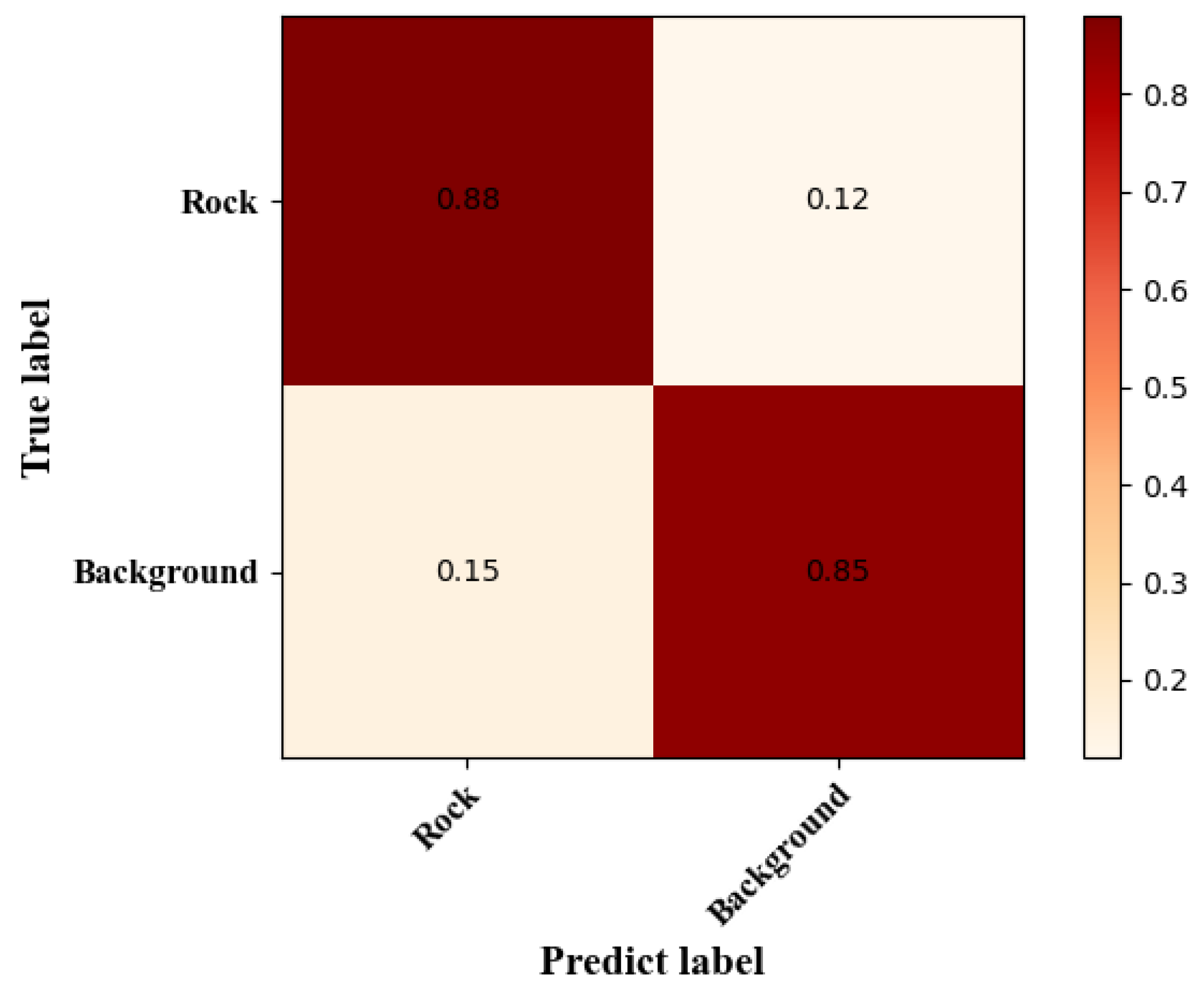
In this paper, the segmentation performance and network model are evaluated using Recall, mean Intersection over Union (mIoU), Accuracy, mean Pixel Accuracy (mPA), and F1 Score. In this study, the segmented particles are considered as positive examples, while the background is treated as negative examples. These metrics are standard evaluation tools in the field of image segmentation, providing insights into the overall performance of the trained model. In binary classification, the four fundamental elements of the confusion matrix are as follows:
TP (True Positive): The model predicts a positive example, and it is actually a positive example.
FP (False Positive): The model predicts a positive example, but it is actually a negative example.
FN (False Negative): The model predicts a negative example, but it is actually a positive example.
TN (True Negative): The model predicts a negative example, and it is actually a negative example.
Figure 12.
Binary Classification Confusion Matrix Result Diagram.
Where:
- (1)
- Recall: It indicates the proportion of correctly predicted positive cases to all positive cases, reflecting the model’s ability to check all cases. The higher the recall rate, the better the model can cover the real positive cases.
- (2)
- mIoU (mean Intersection over Union): is the average value of IoU between multiple classes, which reflects the similarity between multiple classes. the higher the IoU is, the more accurately the model is able to find the locations and ranges of the targets in different classes.
- (3)
- Accuracy: The proportion of true samples in which the model correctly predicts positive examples, reflecting the overall accuracy of the model’s model. The higher the accuracy, the better the model’s ability to predict the overall sample.
- (4)
- mPA (mean Pixel Accuracy): denotes the average of PA for multiple categories, reflecting the model’s correctness in classifying different categories at the pixel level. the higher the PA, the better the model is able to restore the details of different categories of images.
- (5)
- F1 Score :Also known as Balanced F-Score, it is defined as the reconciled mean of accuracy and recall. It is a metric used in statistics to measure the precision of a binary classification (or multi-task binary classification) model. It takes into account both the accuracy and recall of a classification model.The F1-score can be seen as a weighted average of the model’s accuracy and recall, with a maximum value of 1 and a minimum value of 0. A larger value means a better model.
The specific results are shown in Figure 13:
5.2. Loss Function
The stable convergence of loss is one of the key indicators during the model training process, reflecting the optimization effect of the model with the current parameter settings. By observing the changes in the loss curve, the effectiveness of model training can be assessed, and parameters can be adjusted and optimized as needed to further enhance the model’s performance and generalization ability. In this experiment, gradient descent was used as the optimization strategy, adjusting model parameters through repeated iterations to achieve a gradual reduction in the loss function. After 50 epochs of iteration, it was observed that the loss curve gradually stabilized and eventually converged to a minimum value. This indicates that the model achieved a good fit on the training set and can also demonstrate good generalization on the validation set. By analyzing the accuracy and training loss of each epoch, it was found that the loss function gradually converged to a minimum value as the number of training iterations increased, and the accuracy gradually increased with more iterations, as shown in Figure 14 and Figure 15.
5.3. Comparative Tests
To verify the accuracy and generalization capability of the proposed residual network segmentation method incorporating the attention mechanism, multiple comparative experiments were conducted using the same dataset. The models trained using traditional threshold segmentation, DeepLabV3+, Mask R-CNN, and the unmodified U-Net were compared with the improved model presented in this paper. Compared with traditional methods, the proposed method achieved significant improvements in segmentation accuracy, particularly in areas with complex background information and rock main regions. Compared with unoptimized deep learning methods, the proposed model was not only faster in processing speed but also significantly improved the quality of segmentation in rock details. Overall, the experimental data show that the method proposed in this study outperforms existing models in multiple dimensions. It not only speeds up processing but also enhances result accuracy. Table 2 below shows the evaluation metric results after comparative experiments using mainstream image segmentation networks.
For the task of segmenting rock sheet images, the fused attention mechanism proposed in this paper achieves significant performance improvement with the UNet model of ResNet. Recall, mIoU, Accuracy and mPA of the test set are improved compared to the traditional segmentation model. The traditional thresholding segmentation method is ineffective due to the strong dependence on color, especially when facing intricate rock sheet images with similar colors of pores and rock edges.DeepLabV3+, Mask R-CNN network, and the unimproved basic UNet network perform poorly in dealing with the details: the Mask R-CNN network can basically realize the segmentation effect, but it is less effective in dealing with the edges between two rock particles; the basic U-Net network, although it can basically satisfy the processing of the edges of the larger and different mineral particles, can not solve the problem of adhesion between particles of the same characteristics. Although the basic UNet network can basically satisfy the processing of edges of different mineral particles, it cannot solve the problem of adhesion between particles with the same characteristics. The network model proposed in this paper not only solves the adhesion problem between different mineral particles, but also can effectively deal with the adhesion between two identical mineral particles.This network improves the backbone extraction network while enhancing the segmentation accuracy, which makes the model faster and more accurate. This innovative breakthrough is of great significance in the field of rock sheet image segmentation and provides new ideas and methods for related research and applications, and the specific experimental results are shown in Figure 16.
5.4. Ablation Experiments
To analyze the impact of each improvement proposed in this paper on rock thin-section segmentation results, ablation experiments were designed on the same rock thin-section dataset for evaluation. These modules were evaluated under identical experimental conditions to assess their influence on segmentation performance. The ablation experiments were divided into four groups: Group 1 used the U-Net network, Group 2 added the ResNet residual module to the U-Net network, Group 3 added the CBAM attention mechanism to the U-Net network, and Group 4 added both the ResNet residual module and CBAM attention mechanism to the U-Net network. The training parameters used in the experiments were consistent. The specific results of the ablation experiments are shown in Table 3.
As shown in the table above, the UNet model with the added ResNet module shows improvements in both IoU and F1 scores compared to the baseline model, demonstrating better segmentation performance. The UNet model with the added CBAM module also achieves a certain degree of improvement. However, the UNet model that incorporates both ResNet and CBAM modules achieves the best performance, with significant improvements across all metrics. This validates the effectiveness of the residual network module and the CBAM module in enhancing network performance, which is of great importance for image segmentation tasks. These ablation experiment results further confirm the effectiveness and generalization ability of the proposed method, providing valuable reference and guidance for further optimization of image segmentation algorithms.
5.5. Model Generalization Experiment
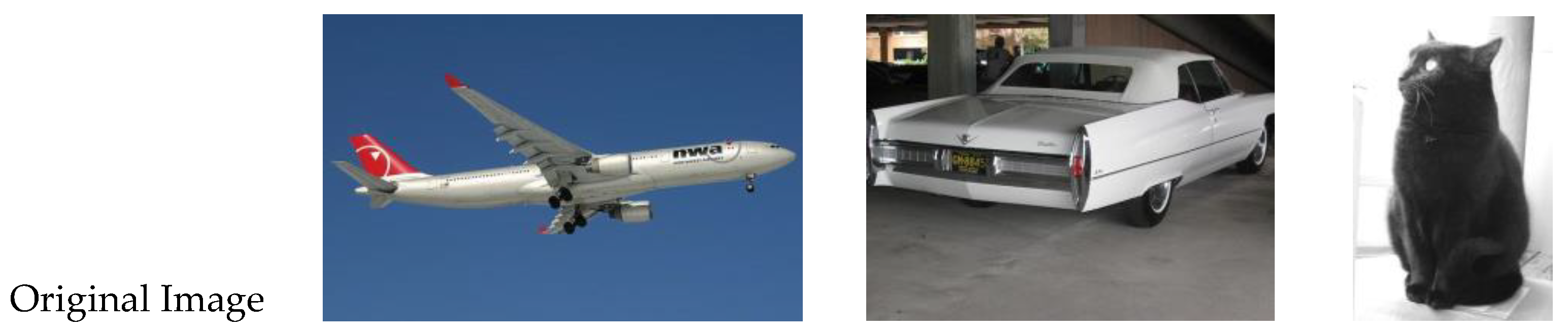
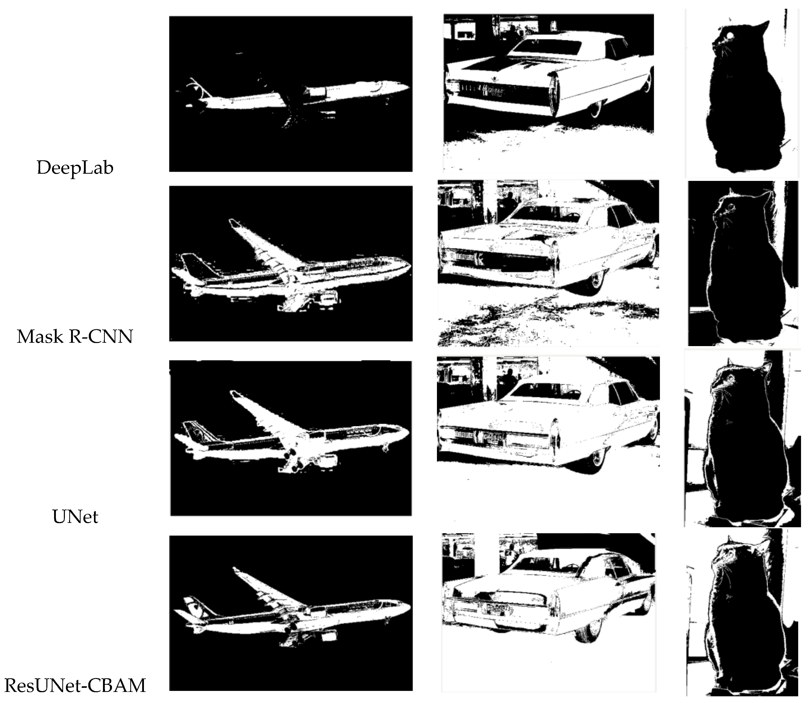
To validate the feasibility and generalization capability of the proposed algorithm model in practical applications, the publicly available PASCAL VOC 2010 dataset was selected for testing. This study compared different algorithms with the effect of incorporating residual networks and adding attention modules. As shown in the figure, the comparison results are displayed. When evaluating model performance, recognizing image details is especially important. In various scenarios, the proposed model demonstrates more accurate segmentation results compared to other methods. For example, it shows high segmentation accuracy for details of airplane wings as well as for textures of steering wheels and tire details in multi-object scenes. This experimental result confirms the robustness and superiority of the proposed method on different datasets, providing strong support for its application in practical scenarios. It further demonstrates the effectiveness of integrating residual networks and attention mechanisms, offering new ideas and approaches for improving the performance of image segmentation algorithms.
Figure 17.
Results of Different Models on the Public Dataset.
6. Conclusions
This paper addresses the issues of insufficient accuracy, poor practicality, and limited generalization capability of traditional rock thin-section image segmentation methods by proposing a novel segmentation approach based on deep learning. Using UNet as the backbone, this method integrates attention mechanisms and residual networks to enable end-to-end automatic segmentation. The increased network depth captures finer feature details, while the attention mechanism enhances the weighting of important feature information, suppressing irrelevant background interference. This improves segmentation accuracy and generalization in cases of complex structures and color inconsistencies. Experimental results demonstrate that this method outperforms traditional approaches across various rock thin-section images, achieving high segmentation accuracy and robustness. However, with increased network depth comes higher computational complexity and longer training times, potentially leading to gradient instability. Future work will focus on further optimizing the network structure to maintain segmentation performance while reducing computational demands, thereby enhancing its practicality and suitability for engineering applications.
References
- Jiang Y, Zhou J, Feng J, et al. Application of DBSCAN Algorithm and Mathematical Morphology in Rock Thin Section Image Segmentation [J]. Microcomputer and Applications, 2016, 35(17): 39-41+48. [CrossRef]
- Li F, Chen M, Zhao Y, et al. Overview of Research Methods for Micro-Pore Structures in Rocks [J]. Groundwater, 2019, 41(06): 112-114. [CrossRef]
- Zhang Z. Research on Sandstone Thin Section Image Segmentation and Recognition [D]. University of Science and Technology of China, 2020. [CrossRef]
- Liu Y, Lü J. Rock Image Segmentation and Recognition Based on Superpixel and Semi-Supervised Learning [J]. Engineering Science and Technology, 2023, 55(02): 171-183. [CrossRef]
- Aligholi S, Lashkaripour G R, Khajavi R, et al. Automatic mineral identification using color tracking [J]. Pattern Recognition, 2017, 65: 164-174. [CrossRef]
- Zhang T, Xu S, Wang Z. Method for Graphic Recognition of Microscopic Pore-Throat Networks in Reservoirs [J]. Journal of Jilin University (Earth Science Edition), 2011, 41(05): 1646-1650. [CrossRef]
- Asmussen P, Conrad O, Günther A, et al. Semi-automatic segmentation of petrographic thin section images using a “seeded-region growing algorithm” with an application to characterize weathered subarkose sandstone [J]. Computers & Geosciences, 2015, 83: 89-99.
- Obara B. A new algorithm using image colour system transformation for rock grain segmentation [J]. Mineralogy and Petrology, 2007, 91: 271-285. [CrossRef]
- Gorsevski P V, Onasch C M, Farver J R, et al. Detecting grain boundaries in deformed rocks using a cellular automata approach [J]. Computers & Geosciences, 2012, 42: 136-142. [CrossRef]
- Long J, Shelhamer E, Darrell T. Fully convolutional networks for semantic segmentation [C]//Proceedings of the IEEE Conference on Computer Vision and Pattern Recognition, 2015: 3431-3440.
- Chen L C. Rethinking atrous convolution for semantic image segmentation [J]. arXiv preprint arXiv:1706.05587, 2017.
- Ronneberger O, Fischer P, Brox T. U-net: Convolutional networks for biomedical image segmentation [C]//Medical Image Computing and Computer-Assisted Intervention–MICCAI 2015: 18th International Conference, Munich, Germany, October 5-9, 2015, Proceedings, Part III. Springer International Publishing, 2015: 234-241.
- Qin X, Zhang Z, Huang C, et al. U2-Net: Going deeper with nested U-structure for salient object detection [J]. Pattern Recognition, 2020, 106: 107404. [CrossRef]
- He J, Feng J, Jiao H, et al. Concrete CT Pore and Fracture Segmentation Method Based on Improved UNet [J]. Journal of China University of Mining & Technology, 2023, 52(03): 615-624. [CrossRef]
- Liang Y, Yi C, Wang G. Building Change Detection in Remote Sensing Images Based on Encoder-Decoder Network UNet3+ [J]. Chinese Journal of Computers, 2023, 46(08): 1720-1733.
- Liu Y, Wu X, Teng Q, et al. Mineral Recognition in Rock Thin Section Images Based on Improved SKnet and Bi-GRU [J]. Intelligent Computers and Applications, 2023, 13(01): 104-111.
- Dong L, Qing L, He X, et al. Core Particle Image Edge Segmentation Algorithm Based on Improved SLIC [J]. Intelligent Computers and Applications, 2021, 11(09): 54-58.
- Li Z, Teng Q, Zhang Y. Particle Segmentation in Orthogonal Polarized Sequence Images of Rock Thin Sections [J]. Modern Computer (Professional Edition), 2018, (03): 26-32.
- Cai Y, Teng Q, Tu B. Automatic Pore Extraction from Rock Cast Thin Section Images Based on Deep Learning [J]. Science Technology and Engineering, 2020, 20(28): 11685-11692.
- He K, Zhang X, Ren S, et al. Deep residual learning for image recognition [C]//Proceedings of the IEEE Conference on Computer Vision and Pattern Recognition, 2016: 770-778.
- Woo S, Park J, Lee J Y, et al. CBAM: Convolutional Block Attention Module [C]//Proceedings of the European Conference on Computer Vision (ECCV), 2018: 3-19.
- Alom M Z, Hasan M, Yakopcic C, et al. Recurrent Residual Convolutional Neural Network Based on U-net (R2U-Net) for Medical Image Segmentation [J]. arXiv preprint arXiv:1802.06955, 2018.
- Abbaszadeh Shahri A, Asheghi R, Khorsand Zak M. A hybridized intelligence model to improve the predictability level of strength index parameters of rocks [J]. Neural Computing and Applications, 2021, 33: 3841-3854.
- Shahri A A, Spross J, Johansson F, et al. Landslide susceptibility hazard map in southwest Sweden using artificial neural network [J]. Catena, 2019, 183: 104225. [CrossRef]
Figure 1.
U-Net network model diagram.

Figure 2.
Comparison of Network Structures.
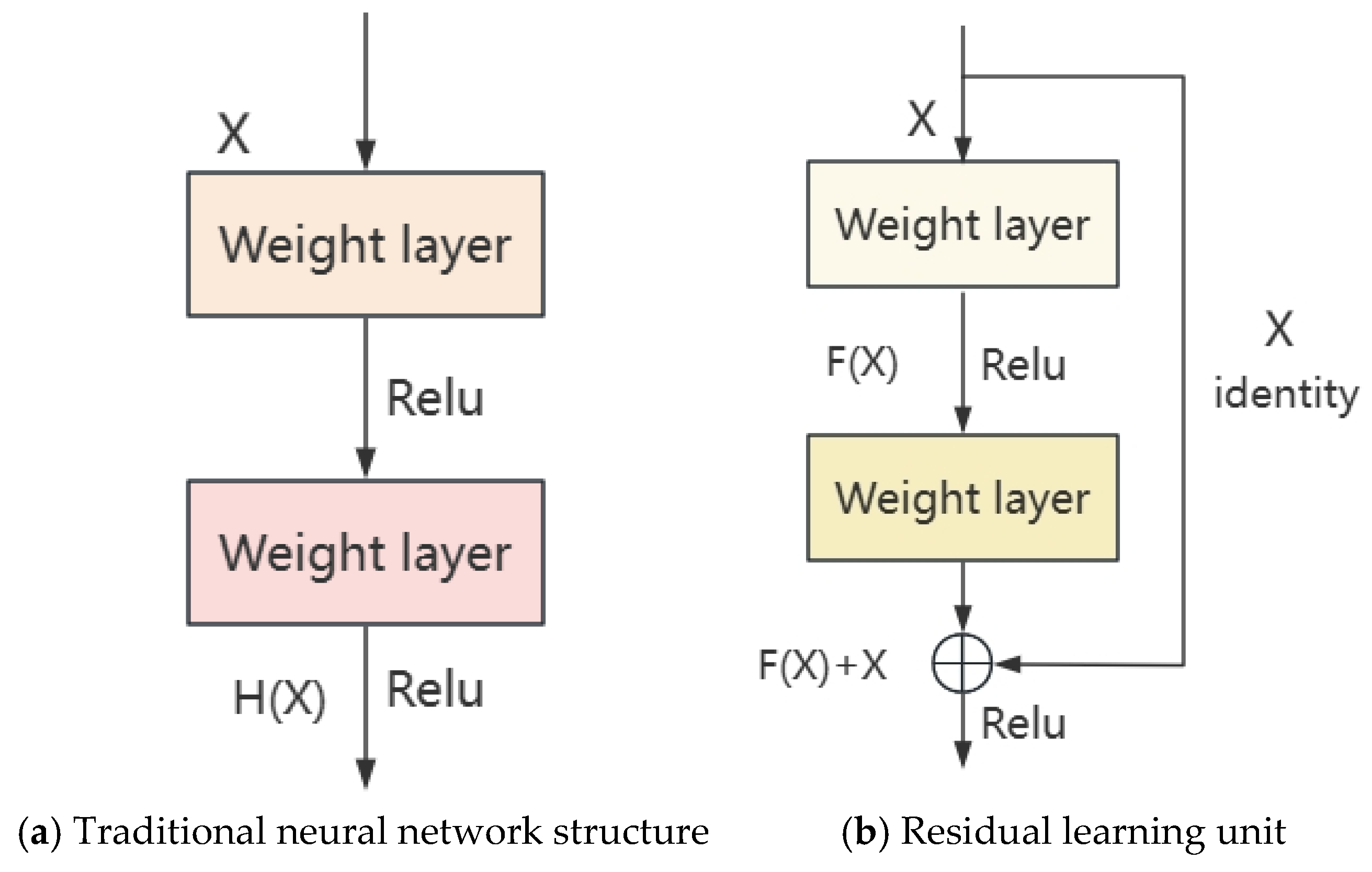
Figure 3.
Structure of the fused residual network at the input of the UNet model.

Figure 4.
Structure of CBAM module.
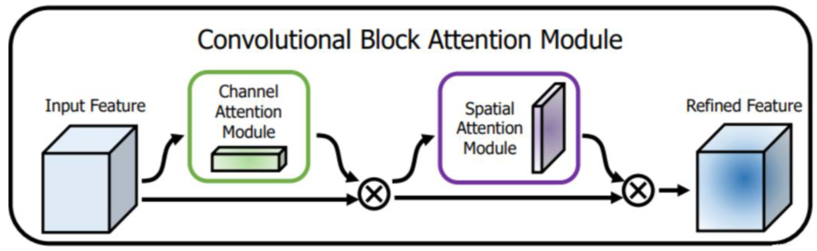
Figure 5.
Channel Attention Module.
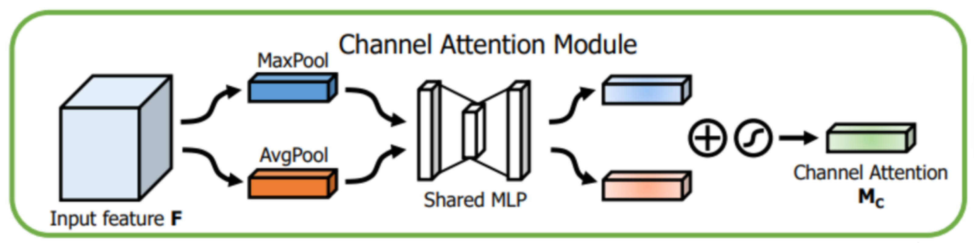
Figure 6.
Spatial Attention Module.
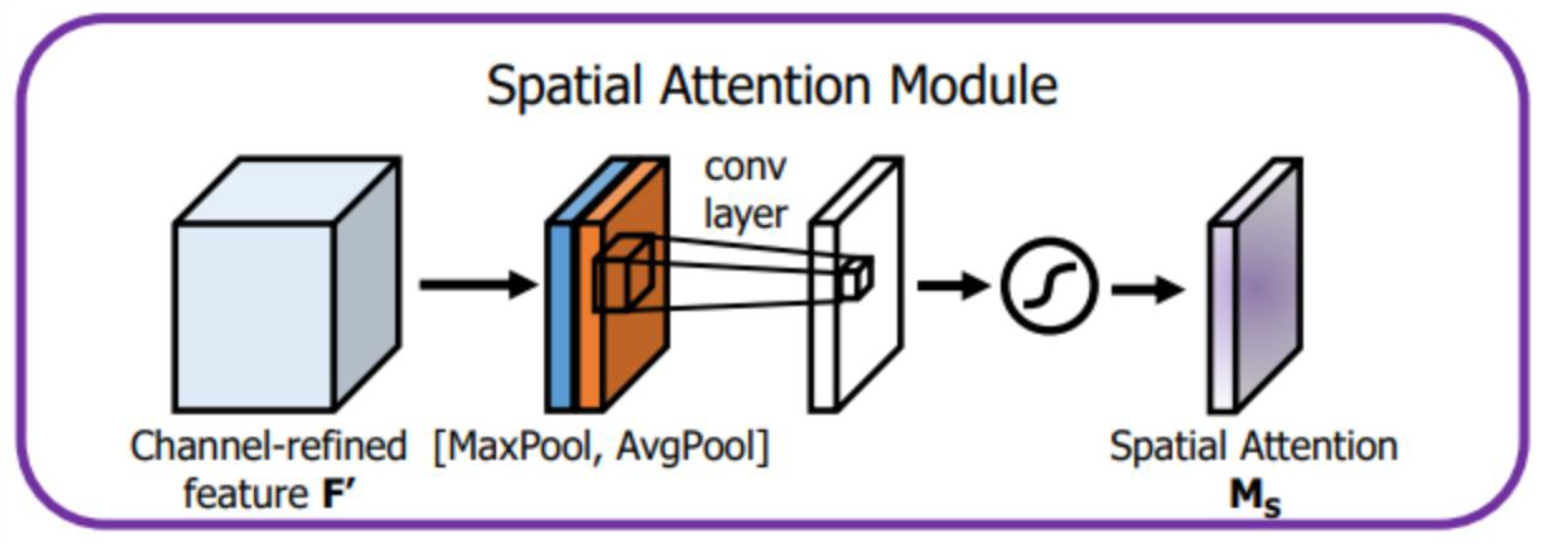
Figure 7.
Residual module.
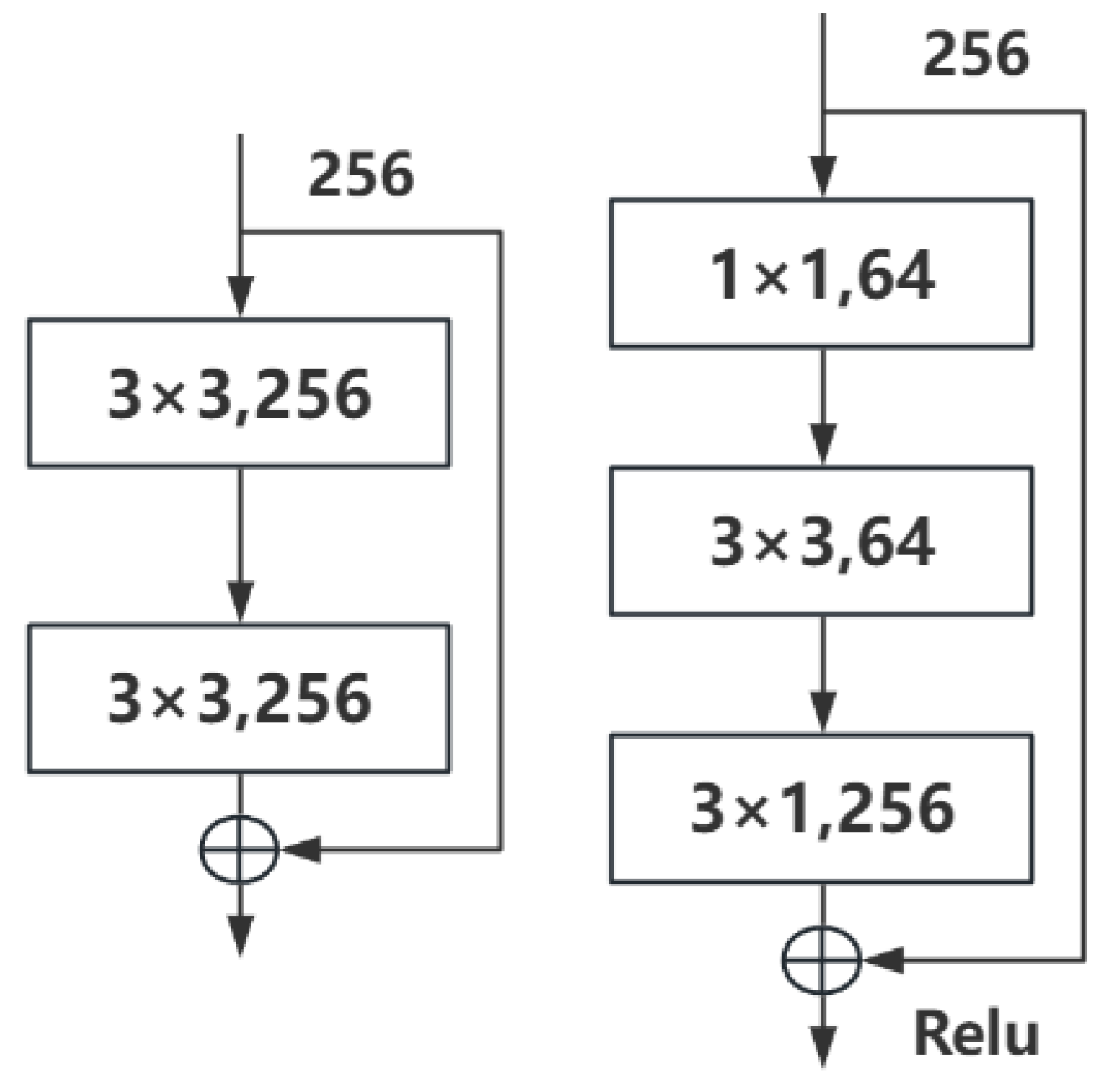
Figure 8.
Model diagram of ResUNet-CBAM network structure.
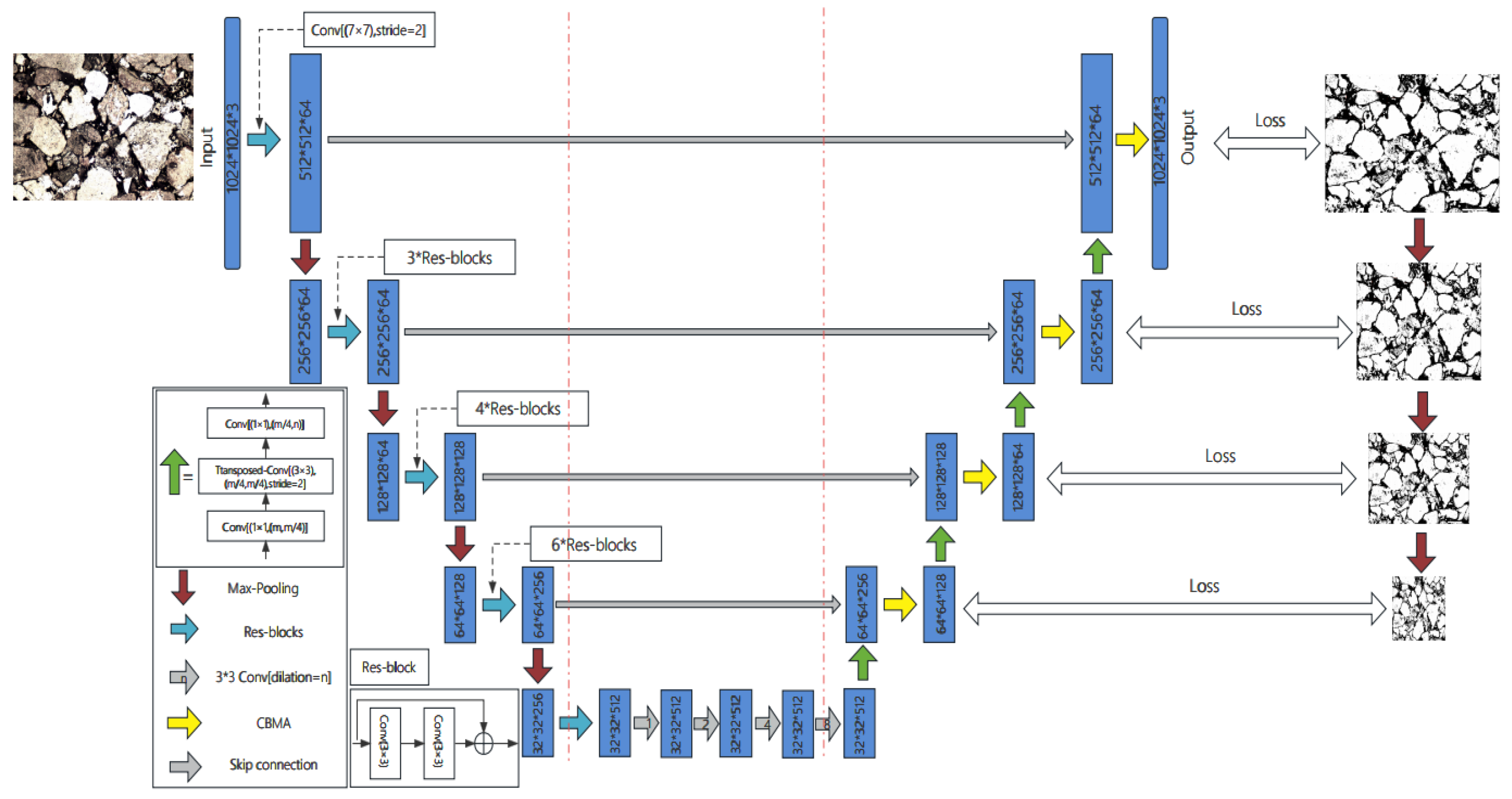
Figure 9.
Data sets.
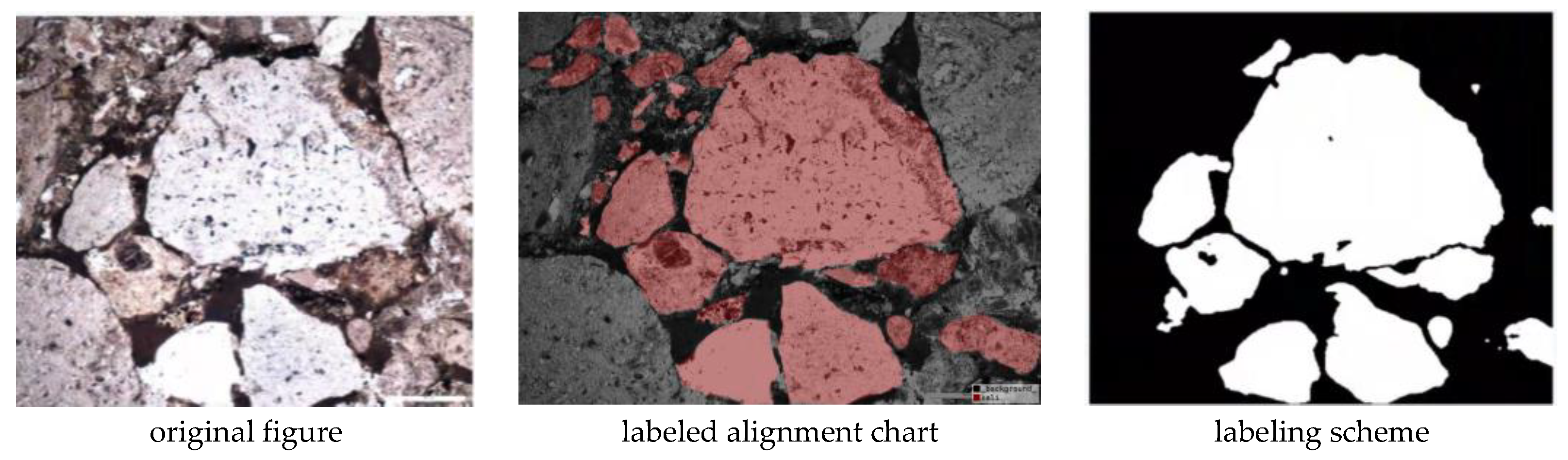
Figure 10.
Comparison of Images Before and After Non-Local Means (NLM) Denoising.
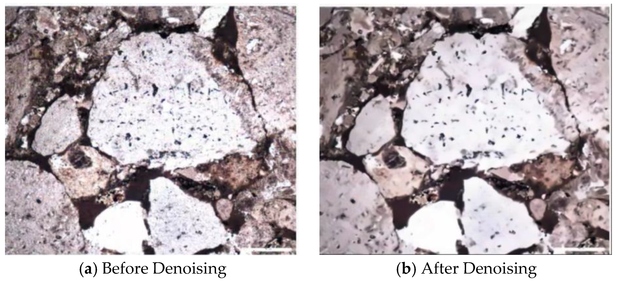
Figure 11.
Common Data Augmentation Methods.
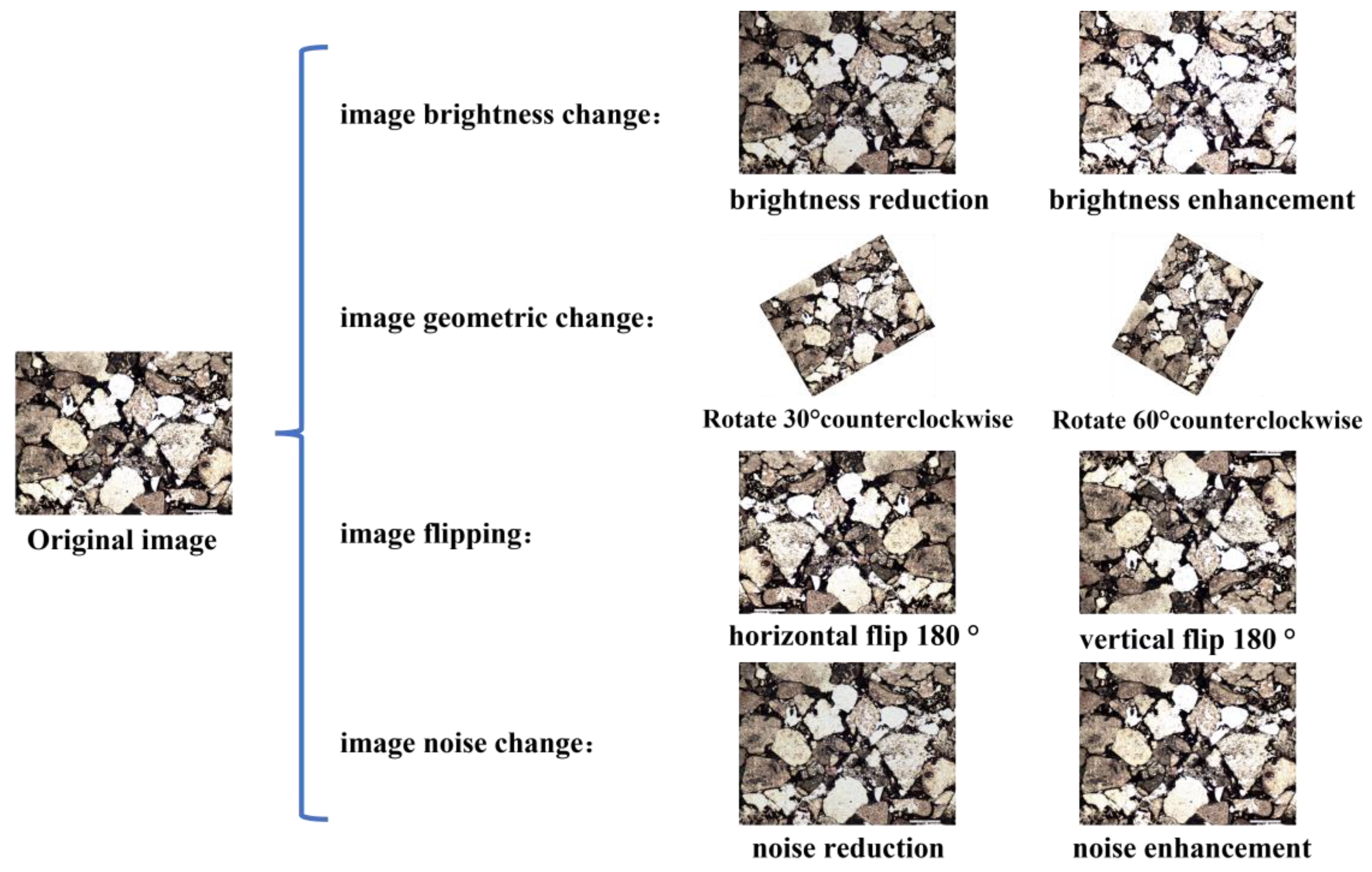
Figure 13.
Graph of model evaluation results.
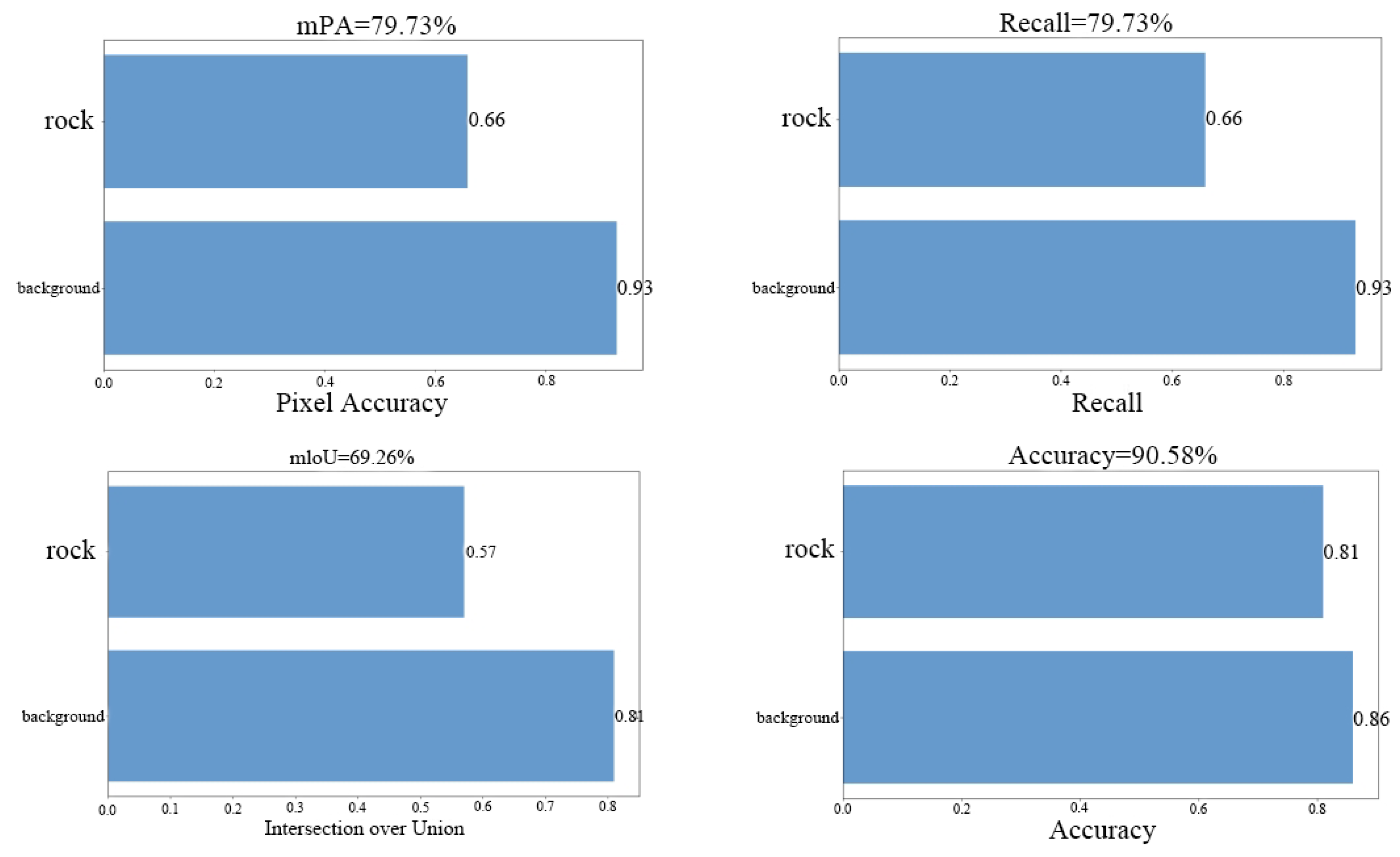
Figure 14.
Training Accuracy Curve.
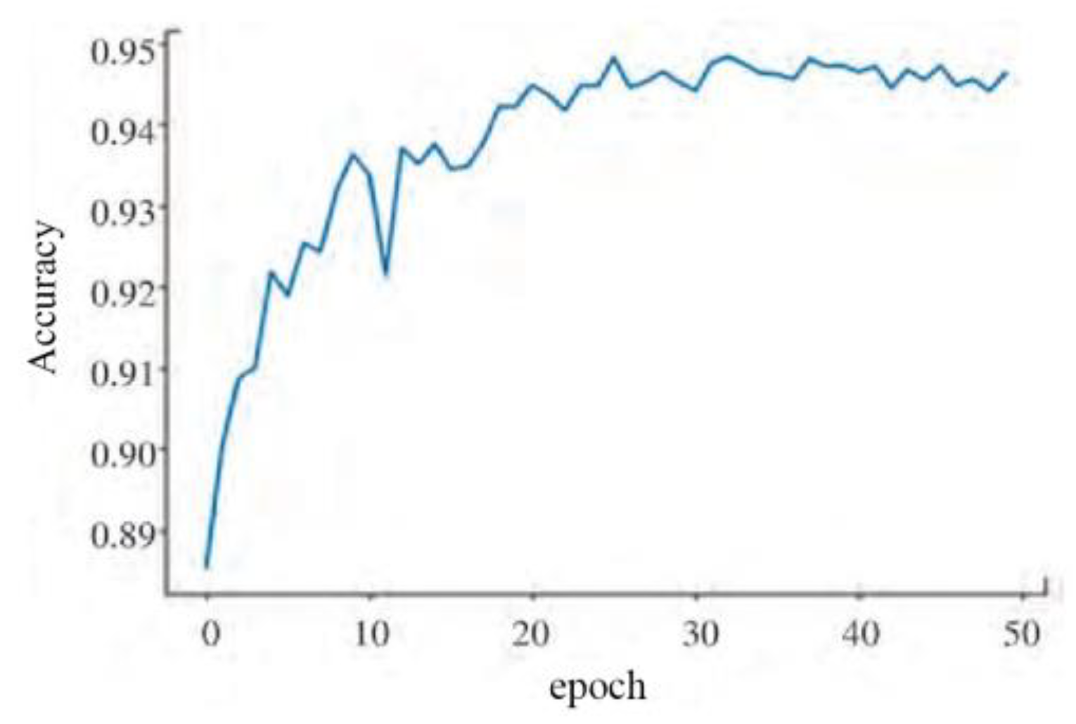
Figure 15.
Training Loss Function Curve.
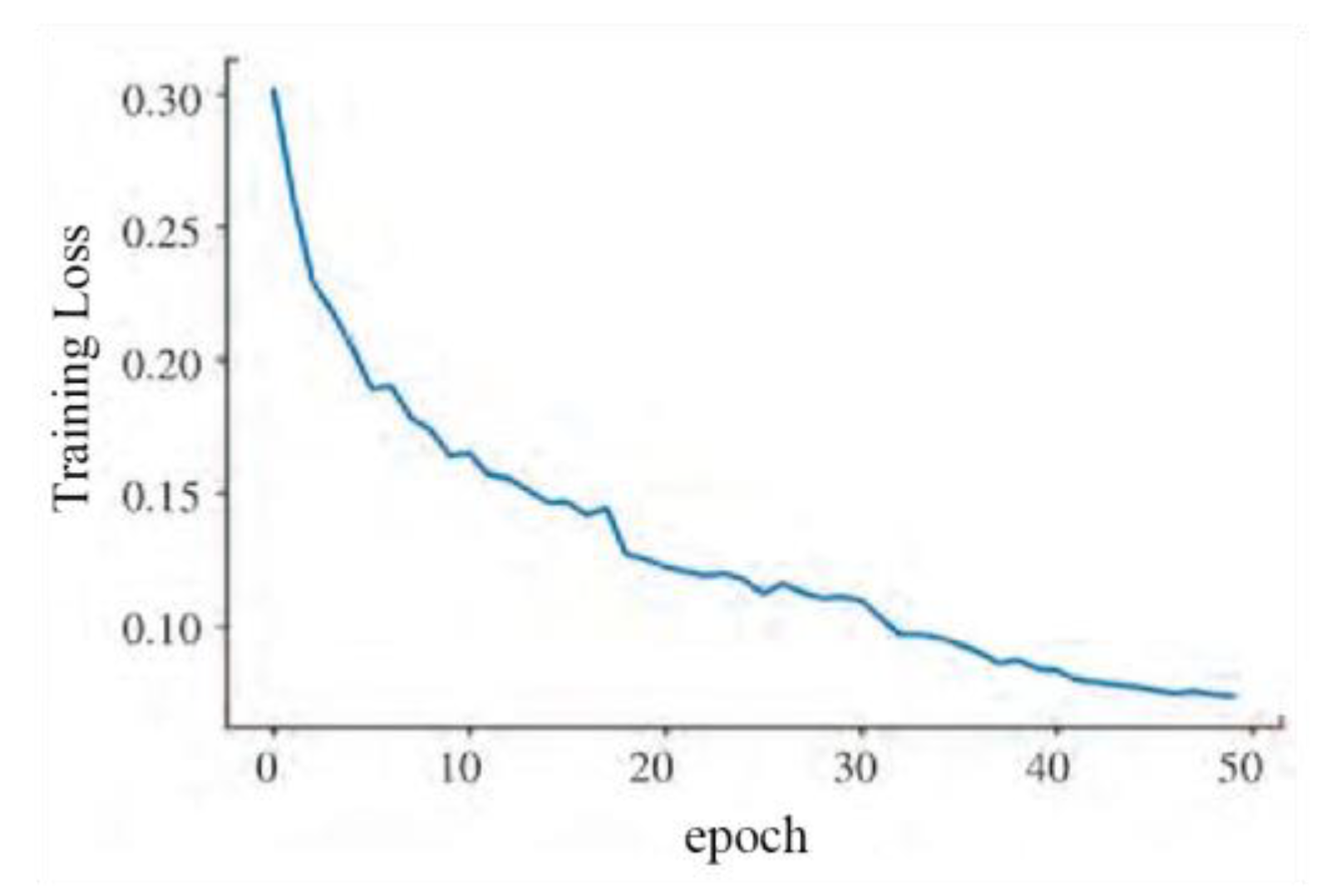
Figure 16.
Segmentation effect diagram of different models.
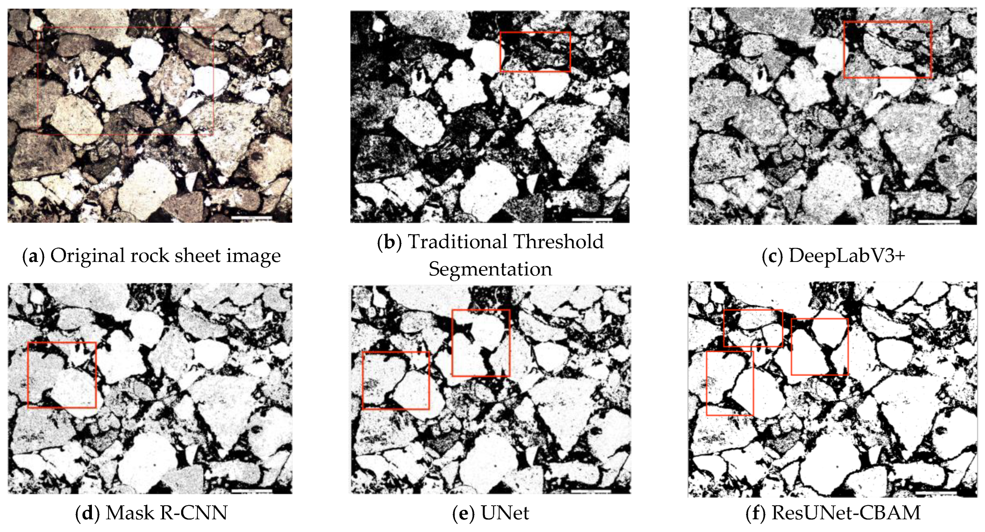

Table 1.
Parameter Settings.
| Parameter name | parameter value |
|---|---|
| Batchsize | 4 |
| learning rate | 1×10⁻⁴ |
| Number of iterations | 100 |
| num_classes | 2 |
| Number of training sets per round | 2400 |
Table 2.
Comparison results of different models.
| Segmentation method | Recall/% | mIoU/% | Accuracy/% | mPA/% | F1 Score |
|---|---|---|---|---|---|
| Traditional Threshold Segmentation | 72.51 | 60.23 | 81.23 | 66.84 | 0.74 |
| DeepLabV3+ | 76.55 | 62.31 | 83.32 | 77.45 | 0.83 |
| Mask R-CNN | 77.01 | 65.89 | 83.56 | 76.32 | 0.79 |
| UNet | 78.93 | 66.23 | 86.92 | 78.25 | 0.80 |
| ResUNet-CBAM | 79.73 | 69.26 | 90.58 | 79.73 | 0.89 |
Table 3.
Results of ablation experiments.
| U-Net | ResNet | CBAM | Accuracy/% | IOU | F1 Score |
|---|---|---|---|---|---|
| √ | - | - | 80.92 | 0.78 | 0.86 |
| √ | √ | - | 82.32 | 0.81 | 0.89 |
| √ | - | √ | 83.56 | 0.80 | 0.88 |
| √ | √ | √ | 90.58 | 0.82 | 0.90 |
Disclaimer/Publisher’s Note: The statements, opinions and data contained in all publications are solely those of the individual author(s) and contributor(s) and not of MDPI and/or the editor(s). MDPI and/or the editor(s) disclaim responsibility for any injury to people or property resulting from any ideas, methods, instructions or products referred to in the content. |
© 2024 by the authors. Licensee MDPI, Basel, Switzerland. This article is an open access article distributed under the terms and conditions of the Creative Commons Attribution (CC BY) license (https://creativecommons.org/licenses/by/4.0/).
Copyright: This open access article is published under a Creative Commons CC BY 4.0 license, which permit the free download, distribution, and reuse, provided that the author and preprint are cited in any reuse.


