Submitted:
28 October 2024
Posted:
29 October 2024
You are already at the latest version
Abstract
Coastal flooding is already one of the most dangerous and costly natural hazards that humanity faces globally and yet it will become even more frequent and challenging to manage because of climate change and other factors. In densely populated estuarine settings, a storm surge barrier is often an attractive and economical solution for flood protection. There are currently many storm surge barriers in operation around the world protecting tens of millions of people and trillions of pounds of property and infrastructure. However, with accelerating rates of sea-level rise being observed, along with changes in storminess, tides and river discharge, surge barriers are closing increasingly often, and closures are now occurring in months when they typically have not occurred in the past. Increased use of surge barriers in the future has critical implications for barrier management, maintenance and operation. In this paper we develop, validate and apply a novel statistical approach to assess how the number of storm surge barrier closures will likely increase in the future and change in frequency throughout the year, that can be used for different climate change scenarios and accounting for forecast errors in water levels. As representative case study examples, we focus on the Eastern Scheldt storm surge Barrier in the Netherlands and the Thames Barrier in the UK. We validate the method, demonstrating it accurately predicts past closure statistics for the Eastern Scheldt and the Thames Barriers over the 38 and 42 years they have been operational, respectively. Then we apply the method to estimate the potential future numbers of barrier closures considering a range of different projections of sea-level rise, along with changes in storm surges, tides and river discharge. We show that there is very likely to be a rapid acceleration in the number of barrier closures in the future, dominated by sea-level rise, with strong influence of the 18.6-year lunar nodal cycle, at both case study barriers. Finally, we illustrate how the tool can be used to help guide future barrier management, maintenance, operation and upgrade/replacement planning and inform adaptative flood management approaches. The tool we have developed could easily be extended to other storm surge barriers around the world.
Keywords:
storm surge barriers
; coastal flood defence
; sea level rise
; climate change
1. Introduction
Coastal flooding, driven by extreme sea levels (e.g., storm surges, waves, high astronomical tides, and relative mean sea level), is already one of the most dangerous and costly natural hazards that humanity faces globally (Jonkman et al., 2024). Yet coastal flooding will become even more frequent and challenging to manage because of: (i) sea-level rise (SLR), changes in storminess (Fox-Kemper et al., 2021) and tides (Haigh et al., 2020a), and land subsidence (Nicholls et al., 2021); (ii) population growth and urban encroachment into flood-prone areas, along with changes in land use and management (McGranahan et al., 2007); (iii) ongoing decline in the extent of natural habitats (e.g., coral reefs, mangroves, and saltmarshes) that act as a buffer to flooding (Committee on Climate Change, 2018); and (iv) ageing assets – in many countries flood defences were built over 50 years ago and are getting more costly to maintain as they age (Haigh et al., 2022).
Major coastal cities are especially vulnerable to coastal flooding, as they often have large and densely populated communities in low-lying areas. Coastal cities have grown rapidly in recent decades, with populations increasing from 360 million in 1990 to 500 million in 2015 (Barragan and de Andres, 2015; MacManus et al., 2021). By 2050, it is likely that more than 800 million people will live in more than 570 coastal cities (WEF, 2019). Hallegatte et al. (2013) estimated that average global flood losses in major coastal cities could increase from approximately US$6 billion per year to over US$1 trillion per year, by 2050, with SLR, subsidence, and socio-economic change, if present flood protection is not upgraded.
Along open stretches of coastlines, building hard and/or soft defences is a typical solution for reducing flood risk (Kamphuis, 2010). However, many coastal cities have built up around estuaries, and in these densely populated areas with long exposed coastlines, space is limited. In a highly developed estuarine setting, the main design choices are to:
(1) Build coastal protection (e.g., dikes) along the shores of the entire estuary (Figure 1a);
(2) Permanently close off the estuary, via a barrage (Figure 1b); or
(3) Temporarily close off the estuary with a moveable storm surge barrier (Figure 1c).
Building coastal protection along the entire shoreline of a large densely populated estuary can be very costly and difficult, due to lack of space and the presence of existing buildings and infrastructure. Permanently closing off an estuary (e.g., the Afsluitdijk in the Netherlands; Janssen et al., 2014) has major implications, for example, for navigation (with ports having to be moved to outside of the estuary), and estuarine ecosystems (as the system moves from brackish to freshwater). Hence, a storm surge barrier is often a more attractive and economical solution for establishing new and/or improving flood protection.
A storm surge barrier comprises a fully or partly movable gate or series of gates that are closed prior to a high water level to prevent flooding behind the barrier (Mooyaart et al., 2017). The gates can then be subsequently reopened to facilitate shipping and allow discharge of water during the low tide and natural movement of tides. There are many surge barriers in operation worldwide today (Walraven et al., 2022), including: the Eastern Scheldt and Maeslant Barriers in the Netherlands (Knoester et al., 1984; Vrancken et al., 2008); the Thames Barrier in the UK (Wilkes and Lavery, 2005); the MOSE Barrier in Italy (Munaretto et al., 2012); the Hurricane Storm Damage Risk Reduction System in New Orleans, USA (Flood Protection Authority East, 2014); and the St. Petersburg Barrier in Russia (Bierawski et al., 2008). Large storm surge barriers are also being considered or planned for Galveston (the ‘Ike dike’; Merrell et al., 2011), New York and New Jersey (Maarten et al., 2019) and Boston (Kirshen et al., 2020) in the US. Storm surge barriers are vital to protecting tens of million people and trillions of pounds of property and infrastructure around the world (Mooyaart et al., 2017).
However, with accelerating rates of relative SLR being observed around the world’s coastline, along with changes in the frequency, intensity and tracks of storms in many locations (which impacts the storm surge, wave, rainfall and river flow climate) (Fox-Kemper et al., 2021), and changes in tides (Haigh et al., 2020a) and river discharge, storm surge barriers are closing increasingly often. For example, over the first 20 operational years (1982/83 to 2001/02; note when referring to a year we use the period from the 31st of July to 30th of June of the following year, to incorporate the main winter storm period), the Thames Barrier in London closed 63 times (33%) to protect the city from flooding; but closed 130 times (67%) over the next 20 years (2002/03 to 2021/22) (Haigh et al., 2020b). Studies of storm surge barriers on the US east coast have also shown increases in closure frequency and variability of closures year to year with increased SLR (USACE, 2019, 2021). Furthermore, seasonal changes are occurring at several barriers with closures occurring during months when they typically did not occur before. For example, in 2020, the Thames Barrier was closed in May to manage flood risk, which had never happened before; historically all other closures of the Thames Barrier have occurred between September and April (Haigh et al., 2020b).
With higher rates of SLR projected in the future and the risk of rapid disintegration of polar ice sheets, along with predicted future changes in storminess, tides and river discharge ( Fox-Kemper et al., 2021), storm surge barriers will be required to close more and more frequently, with an accompanying increase of closures in previously low-risk periods (e.g., summer months, May to August in the case of the North Sea). Increased use of barriers in the future has critical implications for barrier management, maintenance, and operation (Trace-Kleeberg et al., 2023), affecting the integrity/reliability of barriers and their projected lifespan, and putting pressure on the teams that operate surge barriers. Increased use of barriers also has negative ramifications for shipping (increasingly interrupting navigation with economic impacts) and the health of the estuary behind the barrier and the important ecosystems (e.g., saltmarshes) they support. Changes in the months when barrier closures typically occur will have major impacts on the larger maintenance works, upgrading of equipment and testing that is typically scheduled over the low-risk period, which is vital to ensure surge barriers are dependable (Trace-Kleeberg et al., 2023). SLR is very likely to continue to accelerate around the world’s coastline over the coming decades with climate change (Fox-Kemper et al., 2021). Crucially, SLR will continue for hundreds of years, even if we stabilise or reduce our carbon emissions, because it takes many hundreds of years for the cryosphere and the deepest parts of the ocean to adjust to increased air temperature (Clark et al., 2016; Nicholls et al., 2018). It is therefore vital that storm surge barrier operators carefully consider and adapt their management, maintenance and operation to account for climate change, and plan for the major upgrades/replacements that will inevitably be needed in the future.
Therefore, the overall aim of this paper is to develop, validate and apply a statistical approach to assess how the number of storm surge barrier closures will likely increase in the future and vary in frequency throughout the year, to guide storm surge barrier management, maintenance, operation, and upgrade/replacement planning. Our specific objectives are to:
(1) Develop a flexible tool for estimating statistics of storm surge barrier closures in the future, under different climate change scenarios and accounting for forecast error in water levels, and validate the method in a hindcast approach to demonstrate it accurately predicts past closure numbers;
(2) Apply the tool to estimate potential future numbers of barrier closures considering different projections of relative SLR, along with changes in storm surges, tides and river discharge, plus different magnitudes of water level forecast errors; and
(3) Illustrate how the tool can be used to guide adaptative flood management approaches (e.g., Haasnoot et al., 2013), including storm surge barrier upgrade/replacement planning.
As representative case study examples, we focus on the Eastern Scheldt Barrier in the Netherlands (Figure 2a and 2b) and the Thames Barrier in the UK (Figure 2c and 2d); both of which were built in response to the ‘Big North Sea Flood’ of 31st January and 1st February 1953 (McRobie et al., 2005).
The structure of paper is as follows. The two study storm surge barriers and datasets used are described in Section 2. The statistical tool created to estimate potential numbers of closures of storm surge barriers in the future, along with the validation of the approach, is described in Section 3. Assessment of future changes in closure frequencies is presented in Section 4 for a range of different climate change projections and water level forecast errors. A discussion of how the tool can be used to guide adaptative flood management approaches is given in Section 5. Key findings are discussed in Section 6, and conclusions are given in Section 7.
2. Study Sites and Data
2.1. Eastern Scheldt Barrier
Our first case study storm surge barrier is the Eastern Scheldt Barrier, located between the two islands of Schouwen-Duiveland and Noord-Beveland, in the Netherlands (Figure 2a). Built as part of the Delta Works, and in response to the 1953 flood which resulted in the deaths of 1836 people in south-west Netherlands (McRobie et al., 2005), it is one of the largest and most expensive storm surge barriers in the world. It is designed to protect the area around Oosterschelde from extreme sea levels in the North Sea to a 1 in 4000-year design level (Knoester et al., 1984). After the design phase from 1978 to 1982 and construction from 1982 to 1986, the barrier began operating in 1986 and is designed to last more than 200 years. The barrier cost €3 billion (2024 prices) to build. The barrier is a 9 km long concrete dam, with 62 floodgates that are ~42m wide and 6 to 12 m high, each weighing between 260 and 480 tonnes (Figure 2b). When the barrier is open, the flood gates are raised above the water in a vertical position. It takes ~70 minutes to close all gates.
The decision to close the barrier is based on when the water level at the barrier (specifically at the Roompot Buiten tide gauge) is forecasted to rise to 3 m above NAP (Normal Amsterdam Level) (Supplementary Figure S1a). The number of past closures of the Eastern Scheldt Barrier per year and per month are shown in Supplementary Figure S2a and S2b, respectively (including any closures up to 30/06/2024). Note again, when referring to a year we use the period from the 31st of July to 30th of June of the following year, to incorporate the main winter storm period. Over the last 38 years, since it began operation in 1986/87 to the end of 2023/24, the surge barrier has been closed 31 times to protect against extreme water levels (Supplementary Figure S2a), an average of 0.82 closures per year. Some years there have been no closures and the maximum number of closures in a year has been 4 (in 1989/90). All past closures have taken place between September and March with the largest number of closures in October to February (Supplementary Figure S4b).
To assess changes in closure frequency of the Eastern Scheldt Barrier we use water level data at the Roompot Buiten tide gauge, located at the barrier adjacent to the Neeltje Jans Island (Latitude, 51.6195; Longitude, 3.6820), and combine this with the longer record from the nearby OS4 tide gauge (Latitude, 51.6559; Longitude, 3.6940). The water level records were obtained directly from Rijkswaterstaat, the Dutch Ministry of Infrastructure and Water Management, and have a frequency of 10 minutes. The Roompot Buiten tide gauge spans the 37-year period from 15/04/1987 to 31/12/2023 and the OS4 tide gauge spans the period 01/01/1982 to 31/12/2023. Given the two tide gauges are very closely co-located, and measurements of water level are very similar, we combined the OS4 tide gauge record from 01/01/1986 to 15/04/1987, with the Roompot Buiten from 15/04/1987 to 31/12/2023, to create a continuous time series that covers the entire period the Eastern Scheldt Barrier has been operational. Statistics on numbers of past closures of the Eastern Scheldt Barrier were obtained directly from Rijkswaterstaat who own and operate the barrier.
2.2. Thames Barrier
Our second case study storm surge barrier is the Thames Barrier, located in London in the UK (Figure 2c). Like the Eastern Scheldt Barrier, the Thames Barrier was built in response to the 1953 flood which resulted in the death of more than 300 people in south-east England (Wilkes and Lavery, 2005). The Thames Barrier, along with many hundreds of kilometres of sea walls (i.e. dikes) and several smaller barriers and gates, benefits 1.42 million people, £321 billion worth of residential property, 496 education facilities, 711 healthcare facilities, 4 world heritage sites, and designated habitat sites, as well as critical energy, transport and water infrastructure along the Thames Estuary (Environment Agency, 2021). It protects against extreme sea levels from the North Sea and high fluvial flow along the Thames into west London to a 1 in 1000-year design level. Construction began in 1974, and it took 8 years to build. The barrier began operating in 1982, with the first closure in 1983, and is currently expected to be in operation until at least 2070. The barrier cost £1.3B (2024 prices) to build. The barrier spans 520 m across the River Thames. Nine concrete piers divide the river into ten sections ranging from 30 to 61 m, each with a radial gate. Four of the gates sit above the river and make the outer sections non-navigable. The other six gates lie flat on the riverbed, allowing river traffic to pass unimpeded during normal conditions, and they are raised into place during a closure event. The 4 largest central gates are 61 m wide, 20.1 m high and weigh 3,700 tonnes each. It takes ~90 minutes to close all gates.
The decision to close the barrier is primarily guided by a matrix based on forecast water levels at Southend-on-Sea (with consideration of other sites in the Thames Estuary) above ODN (Ordnance Datum Newlyn) and river flow forecasted at Teddington Weir in west London. Note, that to manage the lower order fluvial flood risk in west London, closure decisions are also based on additional secondary spot heights. The closure matrix is confidential; hence we don’t include specific information here, but it is illustrated in Supplementary Figure S1b. The number of past closures of the Thames Barrier per year and per month are shown in Supplementary Figures S2c and S2d, respectively (including any closures up to 30/06/2024). Over the last 42 years, since it began operation in 1982/83 to the end of 2023/24, the surge barrier has been closed 221 times, an average of 5.3 closures per year (Figure 2a). Of those closures, 119 were due to elevated sea levels (e.g., storm surge plus astronomical tide), with 102 closures due to a combination of elevated sea levels and high fluvial flow. Some years there have been no closures and the maximum number of closures per year has been 50 (in 2013/14). All past closures have taken place between September and May with the largest number of closures in December to March (Figure 2b).
To assess changes in closure frequency of the Thames Barrier we use water level data at the Southend-on-Sea tide gauge, located at the mouth of the Thames Estuary (Latitude, 51.5139; Longitude, 0.7255), and river flow data at Teddington Weir in west London (Latitude, 51.4150; Longitude, -0.3088). We merged high-frequency (10 minute) water data from records obtained directly from the Port of London Authority (PLA) and the UK Environment Agency for this site, for the period 1994 to 2023, with historic digitised records of high and low waters captured by Inayatillah et al. (2022) from hand-written tabulated ledgers from the PLA, for the period 1911 to 1994. The final water level dataset spans the 113-year period from 01/01/1911 to 31/12/2023. The river flow dataset was downloaded from the National River Flow Archive (https://nrfa.ceh.ac.uk/data/station/info/39001), it has a daily frequency and spans the 141-year period from 01/01/1883 to 31/12/2023. Statistics on numbers of past closures of the Thames Barrier were also obtained directly from the Environment Agency who own and operate the barrier.
3. Method and Validation
In this section we describe the flexible tool we have developed for estimating the number of surge barrier closures in past and future years, under different climate change scenarios and accounting for forecast error in water levels, and how we have validated the tool to demonstrate it accurately predicts past closures (Objective 1). Our approach has two main stages. First, we use statistical methods to generate artificial but realistic time series of total water level, and for the Thames Barrier, river flow, extending into the future for different climate change scenarios, at the respective sites on which closure decisions are based at both barriers. Second, we then apply the closure rules at each of the two case study barriers in turn on the corresponding artificial future time series, in an adaptable approach that accounts for forecast errors in water levels. These two stages are described in detail in Section 3.1 and Section 3.2, respectively. In Section 3.3, we detail the validation of the tool.
3.1. Generating Artificial Time Series
In the first stage, we generate artificial time series of total water level, with realistic characteristics that match observations, at the two tide gauge sites on which barrier closure decisions are respectively made, namely: Roompot Buiten for the Eastern Scheldt Barrier; and Southend-on-Sea for the Thames Barrier. We use different statistical methods, with parameters fitted to measured historical datasets, to create time series of the three components of still water level (i.e., astronomical tides, storm surges and relative mean sea level) separately, ensuring we accurately reproduce observed temporal variability (e.g., seasonality) and auto-correlation, in each component. We superimpose these time series with climate change projections to generate future time series for different scenarios. Then we combine them to generate records of total water level. We use a Monte Carlo approach to represent intra- and inter-annual variability and therefore to account for uncertainty. Closure decisions for the Eastern Scheldt Barrier are based purely on forecast high water levels at the barrier exceeding 3 m NAP (Supplementary Figure S1a), and so the water level time series at Roompot Buiten are all we need to predict likely closure statistics. However, for the Thames Barrier (as discussed in Section 2.2), decisions to closure the barrier are guided by a matrix, based on both forecast still water levels at Southend-on-Sea and forecast river discharge at Teddington Weir (Supplementary Figure S1b). Hence, we also generate future artificial time series of river discharge at Teddington Weir. The approach we use to generate total water levels is described in Section 3.1.1 and river flow in Section 3.1.2.
3.1.1. Water Levels
Extreme still water levels arise as combinations of: (1) astronomical tides; (2) storm surges; and (3) relative mean sea level (Pugh and Woodworth, 2014). These three components exhibit considerable natural intra- and inter-annual variability. While the tidal component is deterministic, with predictable modulations on fortnightly, monthly, seasonal, 4.4-year and 18.6-year timescales (Haigh et al., 2011), the variability in the storm surges and mean sea-level components is stochastic, with intra-annual (e.g., seasonal) signals and inter-annual variability linked to regional climate cycles (such as the North Atlantic Oscillation; Hurrell, 1995). It is important that our approach realistically reproduces both the temporal variability at different timescales and auto-correlation observed in each of the components, at our two tide gauge sites. Below we describe how we generate artificial time series for each of the three components separately, before combining them to create records of total still water level.
Astronomical tide: First, we generate time series of astronomical tides, at each of the two tide gauge sites, by undertaking a harmonic tidal analysis (on the available measured 10-minute water level data) and prediction, using the U-Tide software tool (Codiga, 2024). For past years, a separate tidal analysis was undertaken for each calendar year, using the standard tidal constituents, to predict the tide for that given year. For years with less than 6 months of data coverage, the tidal component was predicted using harmonic constituents estimated for the nearest year with sufficient data. For the future period, we first undertook a harmonic analysis of the data from the most recent 5 years (2019-2023) and used the standard 68 tidal constituents returned by U-Tide, to predict the tide for all future years from 2024 onwards. Hence, we generate time series of predicted tide (at 10-minute intervals) from the date of the first barrier closure, until a chosen year in the future. Note, when predicting the tides we set the amplitude of the seasonal (SA) and semi-seasonal (SAA) tidal constituents to zero. This is because these are largely driven by non-astronomical processes and these seasonal variations in sea level are represented later in the mean sea-level component, described below.
We predict the tides until the end of 2150. Our tidal predictions accurately capture the variations on daily, fortnightly, monthly, seasonal, 4.4-year and 18.6-year timescales, at each site. As tides are deterministic, we only need a single time series of tidal values at each of the two tide gauge sites. To determine closure statistics, we just need times and heights of predicted high waters (not the full tidal curve), as it is the height of the forecast high water that closure decisions are made on. Therefore, we extract time series of ~twice-daily tidal high waters, using a peaks algorithm (and check that the correct number, between 705 to 708 high waters, are selected each year). Time series of past and future ~twice-daily high tidal levels at Roompot Buiten (Eastern Scheldt Barrier) and Southend-on-Sea (Thames Barrier) are shown in Supplementary Figures S3a and S4a, respectively.
For future scenarios (see Section 4), we start by just considering SLR and assume that tidal characteristics do not change in the future. For these storylines we use the tidal constituents obtained from the harmonic analysis of the 5 most recent years of data, to predict tides into the future (as described above), assuming tidal characteristics remain the same as today. However, an increasing number of studies have observed that tidal levels in many locations have changed and are likely to vary into the future due to non-astronomical factors over seasonal, decadal, and secular time scales (see Haigh et al., 2020a for a detailed review of the topic). Increases in tidal range have been observed at several sites around the southern North Sea, including along the coast of the Netherlands and in the Thames Estuary over the last ~100 years (Jänicke et al., 2000; Haigh et al., 2020a). Therefore, we run additional storylines (see Section 4) in which we account for possible future increases in tidal range, that have been predicted (e.g., Pickering et al., 2017). We do this in a relatively simple way. We use the tidal constituents obtained from the harmonic analysis of the 5 most recent years of data, to predict tides into the future, but each year we increase the M2 tidal constituent by a selected amount (i.e., 1, 2, or 3 mm/yr). We only change the M2 tidal constituent, and no other constituents, because at both tide gauge sites considered here, this constituent is the dominant constituent, as these regions are strongly semi-diurnal.
Skew surges: Second, we generate realistic time series of skew surges, at each of the two tide gauge sites, using an advanced statistical approach, fitted to the historic dataset. Note, we deliberately chose to generate time series of ~twice-daily skew surges and not (10 minute) non-tidal residuals, for two key reasons. Firstly, the non-tidal residual primarily contains the meteorological contribution termed the ‘storm surge’ but may also contain harmonic prediction errors or timing errors, and importantly, non-linear interactions. Non-linear interactions between the tide and storm surge components are particularly large in the southern North Sea (e.g., Horsburgh and Wilson, 2007; Arns et al., 2020). They are complex and vary considerably spatially and are not easily represented in a statistical model. Secondly, as discussed above, closure decisions are only based on heights of high waters, and not the full tidal curve, and so only information at the time of high water is needed. A skew surge is the difference between the maximum observed sea level and the maximum predicted tidal level regardless of their timing during the tidal cycle, and hence each tidal cycle has one high water value and one associated skew surge value. The advantages of using skew surge, instead of non-tidal residual, are that it is: (1) a simple and unambiguous measure of the storm surge relevant to any predicted high water; (2) operationally it defines the quantity relevant to barrier closure decisions; and (3) as Williams et al. (2016) demonstrated, there is negligible dependence between astronomical tide and skew surge, which simplifies our approach, as we can treat the tide and skew surge time series independently (if we generated time series of non-tidal residual, we would have to build an advanced approach to account for non-linear dependence between tide and the non-tidal residual).
Skew surges exhibit strong seasonality, as they are driven meteorologically, and temporal dependence since storm events span multiple tidal cycles. We develop an advanced statistical approach for simulating realistic skew surge time series; this is the first approach, to the best of our knowledge, for simulating realistic skew surge time series that reflect both the seasonality and temporal dependence exhibited in the observed data. To generate time series of skew surges for both past and future years we build on the methodology of D’Arcy et al. (2023), who derived a model for sea levels that uses skew surge and peak tide as two components of sea levels in a joint probabilities framework. They split the distribution of skew surges into extreme and non-extreme values using a peaks-over-threshold framework (Coles, 2001). They use a monthly threshold uj for j = 1, . . . , 12 to account for seasonality, with uj being a quantile, for a fixed percentile, of month j’s skew surge distribution. Using a percentile-based threshold ensures a similar number of exceedances each month. Skew surges below these thresholds are modelled using the monthly empirical distribution to capture within-year non-stationarity of non-extreme values. When tide gauge records have long observational periods, this non-parametric approach can reliably model the main body of the data. For exceedances of the monthly thresholds, they use a generalised Pareto distribution (GPD), which is a well-established model for modelling threshold exceedances (Coles, 2001). This distribution is characterised by three parameters σ > 0, ξ and λ ∈ [0, 1], the scale, shape and rate parameter, respectively. To capture seasonality, they allow the scale σ and rate λ parameter to be dependent on day in year d = 1, . . . , 365 and month j, parameterised by harmonics. For example, for the scale parameter,
for α > β > 0, φ ∈ [0, 365) parameters to be estimated and f = 365 the periodicity. The shape parameter ξ does not vary with any covariate to avoid introducing additional uncertainty typically associated with estimating this parameter.
D’Arcy et al. (2023) account for temporal dependence using the extremal index (Ferro and Segers, 2003). However, this makes simulation difficult and only captures dependence in extreme values. Therefore, here we develop and apply a new approach for accounting for temporal dependence in skew surges. To do so, we use a copula to model dependence of values separated by lag k, assuming the process follows a kth order Markov process. We now describe how we choose the copula model and the value of k to capture temporal dependence. We denote our observed skew surge series as X1, . . . , Xn for n the total number of observations at a specific location. Copulas describe the association between observations separated by some lag k in a series and take different forms; they are commonly used in statistics and extreme value analysis (Nelsen, 2006). We test two different copula models (Gaussian and bivariate logistic extreme value distribution) to contrast the extremal dependence structures (asymptotic independence and asymptotic dependence; Coles et al., 1999). When there is a non-zero probability of Xt+k being large given Xt is large (i.e., exceeding some extreme levels), we say that the series exhibits asymptotic dependence. The Gaussian copula gives a better fit, which agrees with our exploratory findings of asymptotic independence, so there is zero probability of Xt+k being large given Xt is large is zero. This copula is parametrised by a dependence parameter ρ ∈ [0, 1]. We then assume the series follows a kth order Markov process; this is a stochastic process where the distribution a time t is dependent on the distribution at times t − 1, . . . , t − k. The value of k is chosen carefully, by fitting copula models for various values and selecting k based on Akaike and Bayesian information criteria (AIC and BIC, respectively); these are common tools for statistical model selection. We perform this selection at both sites independently, as the storm behaviour can differ. However, we find k = 5 for both sites, corresponding to ~2.5 days. This reflects the known average duration of storm events that typically impact the region (Haigh et al. 2016). Therefore, our model for temporal dependence is characterised by 5 parameters, ρτ ∈ [0, 1] for τ = 1, . . . , 5 representing the strength of dependence for values separated by τ values.
As skew surge records are stochastic, with considerable variability each year, rather than generating a single time series for each of our two tide gauge sites, like for astronomical tides, we generate multiple time series for each site. For Roompot Buiten (Eastern Scheldt Barrier) we generate 500 time series of ~twice-daily skew surge values, at time of high tide, from 1986 to 2150, and an example of a single select record is shown in Supplementary Figure S3b. For Southend-on-Sea (Thames Barrier) we also generate 500 time series of ~twice-daily skew surge values from 1982 to 2150, and an example of a single select record is shown in Supplementary Figure S4b. To demonstrate that our framework generates time series with realistic characteristics that match observations, we compare observed and simulated skew surge datasets for both sites in Supplementary Figure S5. Monthly boxplots of the observed and simulated skew surges are shown in Supplementary Figure S6. Both figures demonstrate that the model does an excellent job of reproducing the observed characteristics, and has the advantage that larger, but still physically plausible skew surges values, are predicted than has been observed in the past.
For future scenarios (see Section 4), we start by just considering SLR and assume that skew surge characteristics do not change in the future. However, we also run additional storylines in which we account for possible future increases in extreme skew surges. To do this we add a year covariate via a linear term to the parametrisation of the scale parameter, assuming mean skew surges change linearly across years. The GPD scale parameter approximates the mean of extreme skew surges, so it makes sense to incorporate long-term increases in storminess through this parameter, although one could also represent changes in the frequency of extreme skew surge events via the rate parameter λ (see D’Arcy et al., 2023). Our updated parameterisation is denoted where is the parameterisation previously defined, y represents the year of interest and is the increase in mean skew surges per year (in metres). For simulation purposes, we specify the value of to create possible future increases in storminess representative of 100%, 200% and 300% changes in skew surges by 2150.
Mean sea level: Third, we generate realistic monthly time series of mean sea level, at each of the two tide gauge sites, and interpolate these to ~twice-daily times of high water. Monthly time series of mean sea level exhibit seasonality, year-to-year variability and a longer-term trend associated with climate change; we aim to capture these variations in our simulations to reflect the realism of the mean sea level component. First, at both Roompot Buiten (Eastern Scheldt Barrier) and Southend-on-Sea (Thames Barrier) tide gauges we compute monthly mean time series of sea level from the observations. We firstly detrend the data-using a quadratic trend to remove long-term trends. Then, we use harmonic analysis to capture the 6-monthly and annual cycles present in the mean sea level. We subtract the fitted seasonal cycle, obtained from the harmonics, from the detrended monthly record, leaving us with a residual time series. We find that it is reasonable to assume this residual time series is independent, and follows a normal distribution, at both sites. Hence, to simulate a realistic mean sea level series, we sample from a normal distribution (with parameters inferred from the fit to the observed data) and add back on the fitted 6-monthly and annual harmonics. This yields a stationary sequence that mean sea-level projections can be added onto.
In the scenarios we run (see Section 4), we use actual annual mean sea level values for the past period at each of the two sites (i.e., 1986 to 2023 at Roompot Buiten and 1982 to 2023 at Southend-on-Sea), calculated from the observations, to capture the observed rise in mean sea level. For the future period we use annual mean sea-level rise projections from the Intergovernmental Panel on Climate Change (IPCC) Sixth Assessment Report (SAR; Fox-Kemper et al., 2021). We offset the projections so that they start from zero in the year 2023. Thus, the simulated time series of mean sea level have; (1) a fitted seasonal cycle; (2) random monthly noise from a normal distribution fitted to the observed data; and (3) annual past mean sea level changes up to 2023 and future projected changes after 2023. Note, for the period 2024 onwards, we use the average mean sea level over the last 5 years (2019 to 2023) as a baseline, upon which we add the annual projections. We use an average of 5 years, rather than one year (i.e., 2023) to represent the future baseline, as annual mean sea level can vary considerably from year to year. Finally, these monthly time series are interpolated to the ~twice-daily high tidal date and times, so they can be combined with the astronomical tide and skew surge time series. For Roompot Buiten (Eastern Scheldt Barrier) we generate 500 time series of ~twice-daily mean sea level values, at time of high tide, from 1986 to 2150, and an example of a single select record is shown in Supplementary Figure S3c, with a high emission SLR scenario (see Section 4). For Southend-on-Sea (Thames Barrier) we generate 500 time series of ~twice-daily mean sea level values from 1982 to 2150, and an example of a single select record is shown in Supplementary Figure S4c, with a high emission SLR scenario.
Total water level: To generate simulated total water level records, we simply combine the single astronomical high tide time series at each site, with one of the 500 skew surge and 500 mean sea level time series. For Roompot Buiten (Eastern Scheldt) we therefore generate 500 time series of ~twice-daily total high water level values, at time of high tide, from 1986 to 2150, and an example of a single select record is shown in Supplementary Figure S3d, with a high emission SLR scenario. For Southend-on-Sea (Thames Barrier) we generate 500 time series of ~twice-daily total high water values from 1982 to 2150, and an example of a single select record is shown in Supplementary Figure S4d, with a high emission SLR scenario.
3.1.2. River Discharge
Closure decisions at the Eastern Scheldt Barrier, are based purely on forecast high water levels (Supplementary Figure S1a), so no time series of river discharge are needed. However, decisions to close the Thames Barrier are based on both forecast still water levels at Southend-on-Sea and forecast river flow at Teddington Weir (Figure Supplementary S1b). Hence, we also generate artificial but realistic future time series of river discharge at Teddington Weir. The daily variation in river discharge over individual storm events, seasons and the longer term is very different to skew surges. For example, auto-correlation operates over much longer periods (days to weeks), and the changes in river discharge over individual storm events are much more asymmetrical, typically with a rapid rise in river discharge followed by a much more gradual decrease, due to the various river catchments draining into the Thames River. This therefore requires a more sophisticated statistical method, than the one we used for skew surges, which is described above. We are in the process of developing an advanced statistical method to capture this variability (see D’Arcy and Tawn, 2024). However, for the purpose of this paper, we took a much simpler approach and just resampled the past dataset. For each future year (note again, a year goes from July to June of the subsequent year to capture a complete winter period), a year from the past between 1883/84 and 2022/23 is chosen to represent that given future year. River discharges are available at daily frequency, and so we use the same value ~twice each day, to correspond with times of ~twice-daily high waters. For Teddington Weir (Thames) we therefore generate 500 time series of ~twice-daily river discharge values, at time of high tide, from 1986 to 2150, and an example of a single select record is shown in Supplementary Figure S4e. Note, we assumed independence between the skew surge and river discharge time series. For the UK east coast, including the Thames region, Hendry et al. (2019) showed that there is negligible dependence between storm surges and river discharge, as the storms that typically generate high skew surges are distinct from the types of storms that tend to generate high river discharge.
For future scenarios (see Section 4), we start by just considering SLR and assume that river discharge characteristics do not change in the future. However, it is likely that future changes in rainfall patterns will influence river discharge in the Thames Estuary and at Teddington Weir (Murphy et al., 2018). Therefore, we run additional storylines (see Section 4) in which we increase the river discharge by different temporally varying percentage changes based on projections from the Environment Agency for the region (Environment Agency, 2022).
3.2. Computing Numbers of Closures and Forecast Errors
To calculate numbers of barrier closures, the tool works by looping through each year in turn, from the year when each barrier became operational (1986/87 at the Eastern Scheldt Barrier; 1982/83 at the Thames Barrier) until 2149/50 and identifies when the closure thresholds are reached or exceeded for each of the 500 total water level (and in the case of the Thames Barrier, the river discharge) time series. By using 500 time series, for each site and scenario, we represent the range of possibilities due to stochastic variability and thereby have an uncertainty envelope. For the Eastern Scheldt Barrier, the number of closures per year are estimated by the number of ~twice-daily total water levels that reach or exceed the closure thresholds in that year (3m above NAP; Supplementary Figure S1a). An example of the number of closures identified for the Eastern Scheldt Barrier, for one of the 500 time series, is shown in Supplementary Figure S3e, with a high emission SLR scenario. For the Thames Barrier, the number of closures per year are estimate by the number of ~twice daily total water levels and river discharges that reached or exceeded the closure matrix (illustrated in Supplementary Figure S1b). An example of the number of closures identified for the Thames Barrier, for one of the 500 time series, is shown in Supplementary Figure S4f, with a high emission SLR scenario. Note again that when referring to a year we use the period from the 31st of July to 30th of June of the following year, to incorporate the main winter storm period in the North Sea.
In the past, the Eastern Scheldt and Thames Barriers (like other storm surge barriers around the world) have been closed on occasions when measured water levels (and river discharge) were lower than the closure matrix. This is because it is the forecast, and not measured water levels at the time, that determine whether the barrier is closured or not. To represent the impact of errors on water level forecasts, and generate more realistic numbers of barrier closures, we use a relatively simple approach within the tool. A forecast error level is defined (in meters). The closure matrix is then lowered by this amount and all exceedances above these lower levels are calculated. This is illustrated in Supplementary Figure S1a for the Eastern Scheldt Barrier, and Supplementary Figure S1b for the Thames Barrier, with a 0.3 m forecast error in water levels. We wrote the tool so that it is flexible, and different closure thresholds and forecast errors can be defined for each year of the simulated period, which allows us to consider adaptative management approaches (see Section 5).
3.3. Validation
We now validate the tool, using a hindcast approach, utilising the 500 simulated time series we have created at each site for the past period (i.e., 1986/87 to 2023/24 at the Eastern Scheldt Barrier; 1982/83 to 2023/24 at the Thames Barrier), considering a range of different water level forecast error levels, and compare predicted closure numbers with those that occurred over the operational period.
For the Eastern Scheldt Barrier, we find the tool best matches observed closure statistics over the 38-year period 1986/87 to 2023/24 when we use a forecast error in water levels of 0.11 m. A histogram showing the range in the total number of closures computed by the tool, over the 500 simulations and the 38-year past period, is shown in black in Figure 3a, and the range in the mean number of closures per year is shown in Figure 3c. In Figure 3a and 3c, blue lines indicate the mean simulated range (across all 500 simulations), and red lines indicate the actual observed number or mean number of closures. Over the 38-year operational period, the Eastern Scheldt Barrier has been closed 31 times, and the tool predicts 31 closures (with a forecast error of 0.11 m), which is excellent agreement. Interestingly, there is a large range across the 500 simulations with the total number of estimated closures varying between 14 and 50 closures, over the 38-year period. This indicates the large range in inter-annual variability that can occur depending on when large skew surges combine with high astronomical tides. Over the 38-year period, the Eastern Scheldt Barrier closed on average 0.82 times per year, and the tool predicts an average of 0.81 closures across the 500 simulations.
For the Thames Barrier, we find the tool best matches observed closure statistics over the 42-year period 1982/83 to 2023/24 when we use a water level forecast error of 0.19 m. A histogram showing the range in the total number of closures computed by the tool, over the 500 simulations and the 42-year past period, is shown in black in Figure 3b, and the range in mean number of closures per year is shown in Figure 3d, overlaid with the 500-simulation average (blue line) and actual observed number (red line). Over the 42-year operational period, the Thames Barrier closed 221 times, and the tool has good agreement, predicting 217 closures (with a forecast error or 0.19 m). Again, there is a large range across the 500 simulations with the total number of estimated closures varying between 146 and 309 closures. Over the 42-year period, the Thames Barrier closed on average 5.3 times per year, and the tool predicted an average of 5.2.
Overall, these results demonstrate the tool can accurately predict past closure statistics at both the Eastern Scheldt and Thames Barriers.
3.4. Future Scenarios
Having demonstrated that the tool accurately predicts past closure statistics, we now use the tool to estimate potential future numbers of closures considering different projections of SLR, changes in storm surges, tides and river discharge, and varying water level forecast errors (Objective 2).
First, we consider just relative changes in SLR, assuming that skew surges, tides and in the case of the Thames Barrier, river discharge, remain unchanged from past/present conditions. We consider 4 SLR scenarios from the IPCC AR6 (Fox-Kemper et al., 2021):
- The 83rd percentile of projection SSP1-1.99, which equates to a low emission scenario;
- The 83rd percentile of projection SSP2-4.5, which equates to a medium emission scenario;
- The 83rd percentile of projection SSP5-8.5, which equates to a high emission scenario; and
- The 95th percentile of the low confidence projection SSP5-8.5, which equates to a high-end (e.g., low-likelihood but high impact) scenario.
We downloaded the local SLR projections for the locations nearest to the Roompot Buiten and Southend-on-Sea tide gauges from the NASA Sea Level Project Tool webpage (https://sealevel.nasa.gov/ipcc-ar6-sea-level-projection-tool). The projections include vertical land movements and are listed in Table 1 for both sites. They are available every decade from 2020 to 2150, relative to a 1995-2014 baseline. We offset each of the 4 chosen projections, so they are zero in 2023 and then interpolate these to the ~twice-daily high-water time series. For the simulations, for both the Eastern Scheldt and Thames Barriers, we assume a rounded water level forecast error of 0.2 m (close to the 0.19 m that gave the best agreement at the Thames Barrier with observed closures; Section 3.3) for consistency and to make it easier to compare statistics between the two study barriers (even though this is larger than the 0.11 m forecast error which gave the best comparison with observed closures at the Eastern Scheldt Barrier; Section 3.3).
The average (solid line) and range (shaded area) of the estimated number of barrier closures, across each of the 500 simulated time series and for each year from 1986/87 to 2149/50, is shown in Figure 4a for the Eastern Scheldt Barrier, for each of the 4 SLR projections considered. The actual number of closures each year that occurred between 1986/87 to 2023/24 are overlaid, as black dots. The average number of closures each year, averaged over each decade from 1990-2000 to 2140-2150, are listed in Table 2. As expected, the number of closures rapidly increases in the future, with SLR. For the high-end SLR scenario (95th percentile of projection SSP5-8.5), the tool indicates that the barrier would close for every single high water just after 2100. For each of the 4 SLR projections, the number of closures of the Eastern Scheldt increases from an average of 1.1, 1.1, 1.1 and 1.1 times per year in 1990-2000, to 2.5, 2.7, 3.1 and 5.3 in 2040-50, to 16, 44, 135 and 654 in 2090-2100, to 122, 411, 667 and 706 times per year in 2140-2150, respectively.
The average (solid line) and range (shaded area) in number of closures each year from 1982/83 to 2149/50 is shown in Figure 4b for the Thames Barrier. The average number of closures each year, averaged over each decade, are listed in Table 2. There is a more rapid increase in the number of closures for the Thames Barrier compared to the Eastern Scheldt Barrier, and a much greater spread across the 500 simulations. This is expected given that the Thames Barrier currently closes around 5 times more frequently each year than the Eastern Scheldt. For each of the 4 SLR projections, the number of closures of the Thames Barrier increases from an average of 4.0, 3.9, 4.0 and 4.0 times per year in 1990-2000, to 24, 26, 31 and 49 in 2040-50, to 108, 180, 298 and 646 in 2090-2100, to 305, 496, 659 and 706 times per year in 2140-2150, for the 4 SLR scenarios considered, respectively. The tidal variation of the 4.4-year perigean and 18.6-year nodal cycle at Southend-on-Sea is shown in Figure 4c (note, the phase is the same at Roompot Buiten, but the magnitude slightly less). Interestingly, as SLR increases over time, the number of closures is more strongly influenced by the 18.6-year nodal cycle, for both the Eastern Scheldt (Figure 4a) and Thames (Figure 4b) Barriers. The number of closures is also influenced by the quasi 4.4-year perigean cycle, but to a lesser extent.
The tool not only captures the number of closures each year, but the date and time when each closure occurs, across the 500 simulations, and so we are also able to examine changes in closure statistics throughout the year. As an example, we show in Figure 5, the dates when closures occurred for the Thames Barrier, for 1 of the 500 simulations, for each of the 4 different SLR projections considered. In these plots each year is on the x-axis and the y-axis shows dates through the year, from January to December. Currently closures typically occur between September and April, for the Thames Barrier (see also Supplementary Figure S2d). However, with future SLR, closures will begin to increasingly occur over the summer months. Closures will start to occur year-round (i.e., every month) from around 2090 in the low-emission scenario, 2070 in the medium-emission scenario, 2050 high-emission scenario and 2050 in the high-end scenario. Again, the plots in Figure 5 show the influence of the 18.6-year nodal cycle, in terms of times of year when closures typically occur.
Second, we consider changes in skew surges. There is little evidence for long-term systematic changes in storminess or storm surge magnitude over the last 100 years above natural variability in the North Sea and around the world (Marcos et al., 2015; Mawdsley and Haigh, 2016; Haigh et al., 2022), although a recent paper challenges this view (Calafat et al., 2022). Moreover, there remains low confidence in future projections of changes in extra-tropical storms or storm surges in the North Sea and globally (Palmer et al., 2018; Fox-Kemper et al., 2021). However, to illustrate that the tool can account for changes in skew surge, and as a sensitivity test, we ran simulations in which we increased the magnitude of the skew surges in time corresponding to 0%, 100%, 200% and 300% increases by 2150. We ran these simulations with the high emission SLR scenario (83rd percentile of projection SSP5-8.5) and a water level forecast error of 0.2 m for both barriers.
The average (solid line) and range (shaded area) in the number of closures each year, for the scenarios in which we have increased skew surge magnitude, is shown in Figure 6a for the Eastern Scheldt Barrier and Figure 6b for the Thames Barrier. The average number of closures each year for the skew surge change scenarios, averaged over each decade, are listed in Table 3. The increases in closures driven by changes in skew surges, are significantly smaller than those driven by SLR. Never-the-less, increases in skew surge magnitude, as expected, drive an increase in closures. Again, as expected the spread of results is larger for the Thames Barrier than for the Eastern Scheldt Barrier. For each of the 4 scenarios considered (i.e., 0, 100%, 200% and 300%), with the high emission SLR scenario, the number of closures of the Eastern Scheldt Barrier increases from an average of 1.1, 1.1, 1.1 and 1.1 times per year in 1990-2000, to 3.1, 4.4, 5.8 and 7.5 in 2040-50, to 135, 163, 187 and 205 in 2090-2100, to 667, 669, 669 and 669 times per year in 2140-2150, respectively. The maximum increase in closures is in the decade 2090-2100 with 28, 51 and 70 extra closures per year for the corresponding 100%, 200% and 300% increases, compared to no increase in skew surges. The number of closures of the Thames Barrier increases from an average of 4.0, 4.0, 3.9 and 4.0 times per year in 1990-2000, to 31, 34, 37 and 39 in 2040-50, to 298, 318, 335 and 349 in 2090-2100, to 659, 663, 664 and 666 times per year in 2140-2150, for the 4 skew surge scenarios considered, respectively. The maximum increase in closures is in the decade 2090-2100 with 19, 37 and 51 extra closures per year for the corresponding 100%, 200% and 300% increases, compared to no increase in skew surges.
Third, we consider changes in tidal range. Often it is assumed tides will remain stationary into the future. However, over the last few decades, a growing number of studies have identified widespread, sometimes regionally coherent, positive and negative trends in tidal levels during the 19th, 20th and early 21st centuries at sites around the world (see Haigh et al., 2020a and references within). Jänicke et al. (2021) identified trends in tidal range in the North Sea of up to several millimetres per year Such changes to tides could therefore impact extreme water levels. Predictions of future changes in tides have been made by, for example, Pickering et al. (2021; 2017) and Schindelegger et al. (2018). As a sensitivity test, we ran simulations in which we increase the tidal range at both barrier sites by 0, 1, 2 and 3 mm/yr. For consistency with other scenarios described above, we ran these 4 simulations with the high emission SLR scenario (83rd percentile of projection SSP5-8.5) and a water level forecast error of 0.2 m for both barriers.
The average (solid line) and range (shaded area) in number of closures each year, for the 4 scenarios in which we have increased tidal range, is shown in Figure 7a for the Eastern Scheldt Barrier and Figure 7b for the Thames Barrier. The average number of closures each year for the tidal range change scenarios, averaged over each decade, are listed in Table 4. The increases in closures driven by changes in tidal range are, like for changes in skew surges, significantly smaller than those driven by SLR. Never-the-less, increases in tidal range, as expected, drive an increase in closures. Again, the spread of results is larger for the Thames Barrier than for the Eastern Scheldt Barrier. For each of the 4 tidal range increases (i.e. 0, 1, 2 and 3 mm/yr) the number of closures of the Eastern Scheldt Barrier increases from an average of 1.1, 1.1, 1.1 and 1.1 times per year in 1990-2000, to 3.1, 3.3, 3.5 and 3.7 in 2040-50, to 135, 156, 177 and 201 in 2090-2100, to 667, 678, 687 and 693 times per year in 2140-2150, respectively. The maximum increase in closures is in the decade 2100-2110 with 32, 64 and 93 extra closures per year for the corresponding 1, 2 and 3 mm/yr increases, compared to no increase in tidal range. The number of closures of the Thames Barrier increases from an average of 4.0, 4.0, 4.0 and 4.0 times per year in 1990-2000, to 31, 33, 34 and 36 in 2040-50, to 298, 316, 335 and 353 in 2090-2100, to 659, 670, 679 and 686 times per year in 2140-2150, for the 4 tidal range scenarios considered, respectively. The maximum increase in closures is in the decade 2090-2100 with 19, 38 and 55 extra closures for the corresponding 1, 2 and 3 mm/yr increases, compared to no increase in tidal range.
Fourth, we consider changes in river discharge, just for the Thames Barrier. Increases in rainfall are predicted to occur in the future over Northern Europe (Palmer et al., 2018), which is likely to drive an increase in river discharge. For the Thames we use projections provided by Environment Agency (2022), from the Maidenhead and Sunbury Catchment, directly upstream of Teddington Weir. Projections are in the form of percentage increases in river flow for the 3 epochs: 2020s (2015 to 2039); 2050s (2040-2069) and 2080s (2070-2125), relative to the 1981 to 2000 baseline, for 4 future emission scenarios, as follows:
- 5.
- No change in river flow;
- 6.
- A central projection based on the 50th percentile, corresponding to a 14%, 17% and 35% increase in river discharge for the 3 epochs, respectively;
- 7.
- A higher projection based on the 70th percentile, corresponding to a 19%, 25% and 47% increase in river discharge for the 3 epochs, respectively; and
- 8.
- An upper projection based on the 95th percentile, corresponding to a 32%, 45% and 81% increase in river discharge for the 3 epochs, respectively;
We interpolated these projections onto the ~twice-daily high-water time series from the start of the year when the two barriers became operational until 2150, extrapolating beyond the third epoch.
The average (solid line) and range (shaded area) of the number of closures each year, for the scenarios in which we have increased river discharge, are shown in Figure 8a for the Thames Barrier. The average number of closures each year for the changes in river discharge, averaged over each decade, are listed in Table 5. The increases in barrier closures driven by changes in river discharge are significantly smaller than those driven by SLR, and smaller than those driven by changes in skew surges and tidal range. Nevertheless, increases in river discharge drive a small increase in barrier closures. For each of the 4 scenarios considered, the number of closures of the Thames Barrier increases from an average of 4.0, 3.9, 4.0 and 4.0 times per year in 1990-2000, to 31, 31, 32 and 32 in 2040-50, to 298, 303, 306 and 312 in 2090-2100, to 659, 663, 664 and 667 times per year in 2140-2150, respectively. The maximum increase in closures is in the decade 2110-2120 with 8, 10 and 18 extra closures per year for the corresponding three scenarios, compared to no increase in river discharge.
Finally, we consider different water level forecast errors, to highlight the important point that the number of times barriers have to close can be decreased by reducing the forecast error. For both study barriers, we ran scenarios with the water level forecast error set as 0, 0.1, 0.2 and 0.3 m. For consistency, we ran these simulations with the high emission SLR scenario (83rd percentile of projection SSP5-8.5).
The average (solid line) and range (shaded area) in number of closures each year, for the scenarios in which we altered water level forecast error, is shown in Figure 9a for the Eastern Scheldt Barrier and Figure 9b for the Thames Barrier. The average number of closures each year for these 4 different forecast errors, averaged over each decade, are listed in Table 6. For each of the 4 water level forecast errors the number of closures of the Eastern Scheldt Barrier increases from an average of 0.4, 0.7, 1.1 and 1.8 times per year in 1990-2000, to 1.2, 1.9, 3.1 and 5 in 2040-50, to 52, 86, 135 and 200 in 2090-2100, to 602, 640, 667 and 685 times per year in 2140-2150. The maximum increase in closures is in the decade 2110-2120 with 78, 159 and 233 extra closures per year for the corresponding 0.1, 0.2 and 0.3 m forecast error, compared to zero forecast error. The number of closures of the Thames Barrier increases from an average of 1.0, 2.0, 4.0 and 8.1 times per year in 1990-2000, to 10, 19, 31 and 49 in 2040-50, to 194, 244, 298 and 352 in 2090-2100, to 609, 637, 659 and 676 times per year in 2140-2150. The maximum increase in closures is in the decade 2090-2100 with 50, 105 and 159 extra closures per year for the corresponding 0.1, 0.2 and 0.3 m water level forecast error, compared to zero forecast error.
3.5. Adaptative Management
In this section, we illustrate how the tool presented here can be used to guide adaptive flood management approaches including storm surge barrier upgrade/replacement planning (Objective 3). We illustrate this by considering the Thames Barrier in London and associated defences.
In 2012, the UK Environment Agency launched the Thames Estuary 2100 (TE2100) Plan to provide strategic direction for the continued management of flood risk in the Thames Estuary through to the end of the 21st century and beyond (Environment Agency, 2012). This Plan was one of the world’s first flood risk management plans to have an adaptive strategy, which embraced uncertainty in future changes in climate change. The plan was adaptive in two ways. First, the Plan was adaptive in that a possible ‘route’ of ‘no regrets’ defence upgrades could be initially followed, with decisions on the most appropriate future pathway, e.g. raising the existing Thames Barrier or constructing a new barrier, being made later as understanding of the rate and risks of climate change improves. Second, the Plan was adaptive regarding the timing of defence upgrades, e.g. raising defences downstream of the Thames Barrier and decision dates for future pathways, can be brought forward if mean and extreme sea levels are found to be increasing faster than predicted. For an adaptive plan to be effective, it must be monitored and regularly reviewed. A monitoring review and a full update of the Thames Estuary 2100 Plan are undertaken every 5 and 10 years, respectively, to determine if it is necessary to alter the flood risk policies, or timing of the actions, outlined in the original Plan. The first monitoring review was completed in 2016 (Environment Agency, 2016) and the first full update was completed in 2023 (Environment Agency, 2023). Within these reviews and updates 10 key indicators are monitored, namely: (1) sea level rise; (2) extreme water levels; (3) river flows; (4) condition of flood defences; (5) Thames Barrier operations; (6) people, property, infrastructure and policy; (7) extent of erosion and deposition; (8) habitat; (9) social, cultural and commercial value; and (10) public and institutional attitudes to flood risk. Following the introduction of the TE2100 Plan, adaptive flood risk management approaches are increasingly being adopted in other locations around the UK and worldwide (e.g. Brisley et al., 2016; Haasnoot et al., 2019).
The operation of the Thames Barrier is one of the 10 key indicators being monitored in the reviews and full updates of the TE2100 Plan. As discussed in the 10-year full update (Environment Agency, 2023) it is vital that the number of Thames Barrier closures are kept within a manageable limit to maintain its reliability and minimise impacts on water quality and river traffic. This is currently set at an average of 50 per year for strategic planning purposes, although the barrier will be closed a greater number of times if required to protect London. The more a barrier closes, the greater the risk of that barrier not being able to operate and there is less time available for maintenance of the barrier and for vessels to navigate through it. As the results in Section 5 have shown, the number of closures of the Thames Barrier could start to reach 50 closures per year as early as 2030’s, due to the peak of the 18.6-year nodal cycle, and exceed an average of 50 closures per year from the 2040s onwards with the high-end SLR scenario, 2050s with the high and medium emission scenarios, and 2060s with the low emission scenario (Figure 4b and Table 2). To reduce the number of barrier closures and keep it within the limit of an average of 50 closures per year, the TE2100 Plan involves reducing the number of combined tidal/fluvial closures, improving water level forecasts (thus reducing forecast errors) and raising defences upstream of the barrier by up to 0.5 m by 2050 and a further 0.5 m by 2090, with a major upgrade/replacement of the Thames Barrier by 2070. We designed the barrier closure prediction tool so that it could be used flexibly, allowing different closure rules and water level forecast errors to be defined for different years, and our tool was used to assess and guide decisions in the 10-year review of the TE2100 Plan.
To illustrate the way in which we can use the tool to guide adaptative flood management of surge barriers, we have run example simulations in which we alter the closure matrix for the Thames Barrier. For the period 1982/83 to 2049/50 we use the existing closure matrix, an illustration of which is shown by the solid line in Supplementary Figure S7. For the period 1950/21 to 2089/90 we increase the water level height of the closure matrix by 0.5 m. This corresponds with a planned 0.5 m raise in tidal defences upstream of the barrier, completed by 2050 (Environment Agency, 2023). We also adjust the matrix, to reduce the number of combined tidal/fluvial closures, by increasing the river discharge thresholds, for higher discharge values, relative to the water level. This modified closure matrix is illustrated by the dotted line shown in Supplementary Figure S7. For the period 2090/91 to 2149/50 we increase the water level height of the closure matrix by a further 0.5 m (1.0 m relative to the original closure matrix), corresponding with a planned further 0.5 m rise in tidal defences upstream of the barrier, completed by 2090 (Environment Agency, 2023). This modified closure matrix is illustrated by the dashed line shown in Supplementary Figure S7. The number of estimated barrier closures, across all 500 simulations, is shown in Figure 10, assuming a high emission SLR scenario (83rd percentile of projection SSP5-8.5), no change in tidal range, skew surge or river discharge and a water level forecast error of 0.2 m. The average number of closures of the Thames Barrier increases and reaches an average of 50 closures per year, just prior to 2050. However, with the first modified closure matrix (corresponding to a 0.5 m increase in the height of defences upstream of the barrier by 2050 and the reduction in combined tidal/fluvial closures), the number of closures reduces back to average levels observed between 1982/83 and 2023/24. With SLR accelerating, the number of closures increases back to an average of 50 closures per year, prior to 2090, but then subsequently reduces back to present/day average levels, when the second modified closure matrix is used, before increasing again to an average of more than 50 closures just prior to 2120. The two raisings of upstream defences, along with the reduction in combined tidal/fluvial closures, would essentially buy time, allowing the barrier to continue to efficiently function and be maintained. In the original 2012 Plan, the raising of the upstream defences was planned for 2065 and 2100, but was brought forward to 2050 and 2090, reflecting the results presented here. This therefore illustrated the flexibility of the tool, and because it is computationally efficient it can be used to quickly run a wide variety of different scenarios within an adaptive framework.
4. Discussion
In this paper we have described the development of a novel and flexible tool which can be used to assess how the number of storms surge barrier closures will alter in the future with different climate change scenarios and vary in frequency throughout the year, to guide storm surge barrier management, maintenance, operation and upgrade/replacement planning. We have demonstrated, using the Eastern Scheldt and Thames Barriers as examples, that the tool accurately predicts the correct number of closures that have occurred over the period that both barriers have been operational. Our tool can be used to consider different projected changes in SLR, skew surges, tidal range and river discharge, while accounting for water level forecast errors. We have demonstrated that our tool is flexible, and thus can be used to assess adaptive management approaches for storm surge barriers. Furthermore, the tool is computationally inexpensive and provides an uncertainty range in estimates, by using a Monte Carlo approach to represent intra- and inter-annual variability.
We have applied the tool to estimate potential future numbers of barrier closures considering a realistic range of different projections of SLR, along with sensitivity to changes in skew surges, tides and river discharge. We find that the dominant driver for increases in barrier closures in the future, is SLR, with much more modest changes in closure numbers likely to be associated with increases in skew surges, tidal range and river discharge. With SLR there is a rapid acceleration in the number of barrier closures. In the future, as SLR accelerates, the number of closures each year becomes increasingly influenced by the 18.6-year nodal cycle in astronomical tides, and to a lesser extent by the quasi 4.4-year perigean cycle. This is because SLR raises the baseline and increasingly closures are caused by just high spring tides; a storm surge is no longer necessary to raise levels to the closure thresholds. As expected, the rapid acceleration in the number of barrier closures due to SLR, and increased influence of the nodal cycle as high sea levels are driven by high spring tidal levels, matches the results of recent studies that have identified a rapid increase and nodal modulation in so-called nuisance, sunny day or high tide flooding (e.g., Ray and Foster, 2016; Moftakhari et al., 2017; Jacobs et al., 2018; Sida Li et al., 2021; Thompson et al., 2021; Hague et al. 2022).
These results are important because barrier operators have long-term plans (often many decades in advance) of when they are going to do major maintenance jobs and upgrades. We are already starting to use this tool, to help barriers in the UK and the Netherlands consider whether they should move the scheduling of large maintenance jobs backwards or forwards in time, to align with troughs on the 18.6-year nodal cycle when fewer closures are expected so that maintenance work is not as frequently interrupted by barrier operations. Our results also show that with SLR there will be changes in the months when barrier closure typically occur, with more and more closures over the low-risk season (May to September in the North Sea). The aforementioned first observed closure of the Thames Barrier in May 2020 is a sign of things to come, an early warning that changes are already happening. This is vitally important, as it will significantly reduce the time available for the maintenance work, upgrading of equipment and testing that is often scheduled over the low-risk period. In addition, and in relation to water safety requirements, it is also important to consider that during major maintenance projects in low-risk period, some barriers are sometimes temporarily unavailable or only partially available for several subsequent weeks or even months. Other barriers (e.g., the Thames) are always operational, even within major maintenance periods, but closures during maintenance periods disrupt work, causing significant delays and increase costs with sometimes unforeseen knock-on effects. Therefore, barrier operators will be required to radically change the way maintenance is planned and carried out to guarantee barrier are operational and maintain their reliability. Budgets for maintenance will have to be increased. There will also be more pressure on staff, as the number of operations increases. Furthermore, increased barrier closures will have negative ramifications for shipping (increasingly interrupting navigation with economic impacts) and the health of estuarine ecosystems (as increased closures will affect the salt and freshwater mixing regime). Trace-Kleeberg et al. (2023) discuss these issues in more detail. Further work is needed to assess these issues thoroughly, and crucially to determine tipping points when actions to manage closure numbers are required, e.g. raising of fixed defences upstream of the barrier, or ultimately when it will be necessary to move to a barrage. As we have shown (Figure 10), adaptative management solutions can be developed and applied to reduce the number of closures. However, these solutions (e.g., raising defences upstream of the barrier) are very costly, and only buy time. As many new surge barriers and barrages are being proposed to deal with projected SLR, more systematic investigations and guidance on the merits and demerits of surge barriers and barrages would be helpful.
Results have also shown (Figure 9) that improving water level forecasts will reduce the number of times barriers have to closure. Therefore, as the rate of SLR continues to accelerate, reducing forecast error should be made a priority. Teams in both Rijkswaterstaat and the UK Environment Agency, are currently conducting collaborative studies with this aim. With further optimization of the forecasting models, an error of 10 cm may be a realistic target value and will result in significant less barrier closures. Recent advances in Machine Learning (MI) and Artificial Intelligence (AI) offer exciting possibilities for enhancing forecasting and reducing errors. However, reducing forecast errors will only buy time as rates of SLR continues to accelerate.
We have demonstrated that our new tool can estimate numbers of barrier closures expected under different SLR projections, along with sensitivity to changes in skew surges, tides and river discharge, considering different forecast errors, and is flexible allowing different closure thresholds and forecast errors to be defined for different periods. Along with using a low-, medium- and high-emission SLR scenario, we have also considered a low-likelihood but high impact SLR scenario. There is low certainty in this scenario, particularly due to uncertainty in the rate of thinning and mass loss from Antarctica. Changes in sea level recorded in the geological record suggest that there may be dynamic processes currently not accounted for in many climate models, which may drive rapid ice sheet loss and therefore SLR with the potential to impact the high-end, particularly beyond 2100 (Kopp et al., 2017). Here we follow the IPCC AR6 and utilise the 95th percentile of the SSP5-8.5 projection, but due to this uncertainty, there are diverging views on these worst-case physically plausible high-end sea-level scenarios (e.g., Bamber et al., 2019; van de Wal et al., 2022). Adaptive flood risk management embraces this uncertainty and permits flexible decision-making, depending on the uncertainty tolerance of the user, as the scientific evidence increases.
In our approach, we have deliberately used relatively simple approaches to represent changes in skew surges, tides and river discharge, but more advanced approaches could be developed and integrated into the tool. For example, when assessing changes in tidal range, we simply change the M2 tidal constituents for simplicity and no other constituents, because at both tide gauge sites considered here this constituent is the dominant one, as these regions are strongly semi-diurnal. In areas of mixed or diurnal tidal characteristics, other tidal constituents could be altered to achieve the same effect, or a more sophisticated approach could be developed.
We have assumed independence between skew surge and river discharge for the Thames Barrier, as Hendry et al. (2019) showed there is negligible dependence between storm surges and river discharge along much of the UK East Coast including in the Thames Estuary. However, for barriers where there is strong dependence between skew surge and river discharge, this could be relatively easily accounted for, by using, for example, copula functions. We have also assumed independence between tide and MSL at our two case study locations, which is a reasonable justification given the year-to-year variability in MSL is very small compared to tidal range. However, in some other locations, particularly in regions when MSL variability is larger, and tides are smaller, tides can be influenced by MSL variations (see e.g., Devlin et al., 2017). Furthermore, at our two study sites we found that the monthly MSL residual values (after removing the MSL seasonal cycle) were independent from each other, and therefore can be represented well by a normal distribution. However, in other regions, particularly those dominated for example by El Niño–Southern Oscillation (ENSO), monthly MSL residual values are likely to be highly correlated (see e.g., White et al., 2014). Again, our approach could be adapted to account for both these influences. Finally, at each of the two case study barriers, heights of waves do not influence the closure decisions, and therefore we did not consider waves in this paper. However, the method could be relatively easily extended to include waves at other barriers, if needed.
In this study, we have estimated past and future closures of the Thames Barrier using the matrix based on forecast water levels at Southend-on-Sea and river flow forecasted at Teddington Weir in west London. However, to manage the lower order fluvial flood risk in west London, closure decisions are also based on additional secondary spot heights. For simplicity we have not accounted for these secondary sites here, as many are upstream of the barrier and past water level measurements are impact by previous barrier closures. The vast majority of the 50 barrier closures in 2013/14 were to manage fluvial flood risk in west London; our method therefore underestimates past closures in this particular year (Figure 4d), because we don’t explicitly account for them. However, our approach could be extended to account for these types of closures, and this is something we hope to do in a future study.
Just prior to completing this study, we learnt of the earlier and ongoing work of O’Brien (2017). In his PhD thesis, he developed an approach to estimate closures of the Stamford Hurricane Barrier in Connecticut (USA). O’Brien’s statistical approach is very different to the one we have undertaken here. His approach uses historical daily water level maximums and produces monthly probability density functions (PDF). The logistic distribution was selected for the Stamford Hurricane Barrier water level data based on best fit criteria. SLR projections are added to the location parameter, which shifts the monthly PDFs to the right. His approach uses a Bernoulli process to create 100 random draws each day from the SLR adjusted PDFs. A stepwise operational exceedance curve is created using historical operational probabilities, and accounts for closure uncertainties, which can be attributed using closure data records to hydrometeorological or other factors. A perfect foresight operational curve is created to determine excess closures from uncertainty, and used to create a threshold exceedance model, which counts and aggregates closures and excess closures. Because his approach is based on total water level (and tides are not represented separately), future predictions of closure numbers are smoothed and do not account for the nodal cycle explicitly like we do here. However, like our study, his results show a rapid acceleration in gate closures with SLR, with estimates of closures of the Stamford Hurricane Barrier roughly consistent with results from our two barriers, for the low, medium and high emission scenarios he used. Our approach also has the added advantage that it considers ~twice-daily high waters, and not the single peak high water each day like O’Brien’s approach (2017). However, O’Brien includes a more sophisticated approach for accounting for errors in water level forecasts, represented by the use of operational curves, than the simplistic approach we have taken. Our current approach, rather than realistically simulating forecast errors, is essentially a tuning parameter to best match past closure statistics. Whereas O’Brien’s approach is to fit a conditional probability distribution (CDF) to the operational closure records and apply that to his synthetic daily peak water levels, to determine closure numbers. In future work, we plan to update our approach and follow the more sophisticated method of O’Brien to account for water level forecast errors. We also plan to carry out a detailed comparison between our and O’Brien’s approach, using exactly the same climate change projections.
We have just considered just the Eastern Scheldt and the Thames Barriers here, but our tool can easily be extended to other storm surge barriers worldwide. All that is needed to apply the tool to other barriers is closure thresholds and observation datasets. We have recently tested the tool for other barriers in the UK, Netherlands and USA, and it is able to accurately predict past closure statistics at these other barriers. In addition, the approach we used to generate synthetic time series of high sea levels, with realistic temporal characteristics that match observations, could be used much more widely in a range of applications to inform coastal flood risk management.
5. Conclusions
In this paper we have described a flexible tool we have developed for estimating the likely number of closures of storms surge barriers in the future, and the frequency of closures throughout the year, under different climate change scenarios and accounting for water level forecast errors. We validated the method, demonstrating it accurately predicts past closure statistics for the Eastern Scheldt Barrier in The Netherlands and the Thames Barrier in the UK. Then we applied the tool to estimate potential future numbers of barrier closures considering different projections of SLR, along with changes in tides, storm surges and river discharge, accounting for different water level forecast errors. We showed that there is likely to be a rapid acceleration in the number of barrier closures in the future, with the strong influence of the 18.6-year nodal cycle. Increases in barriers closures is dominated by SLR, with much more modest changes resulting from increases in skew surges, tidal range and river discharge. Finally, we illustrated how the tool can be used to help guide future barrier management, maintenance, operation, and upgrade/replacement and inform adaptative flood management approaches. For example, raising defence upstream of the barrier, can be used to reduce the number of barrier closures in the future and buy time. The tool we have developed could relatively easily be extended to estimate changes in closure numbers of other storm surge barriers around the world.
Supplementary Materials
The following supporting information can be downloaded at the website of this paper posted on Preprints.org.
Author Contributions
I.D.H and JB conceptualized the study. The methodology was developed by I.D.H and E.D and reviewed by all the other authors. Data was provided by K.S. and L.C. The first draft of the paper was written by I.D.H. All other authors reviewed the paper and provided feedback.
Acknowledgments
We would like to thank Jonathan Tawn for his useful feedback on the statistical approaches applied here. IDH time on this projected was primarily funded by the Environment Agency and a UK Natural Environment Research Council (NERC) Knowledge Exchange fellowship grant UPSURGE (NE/V018655/1), but also contributes to the NERC funded ISOTIPIC project (NE/Z503344/1). This paper also forms a contribution to the RISeR project, which has received funding from the European Research Council (ERC) under the European Union’s Horizon 2020 research and innovation programme (grant agreement no. 80228); supporting IDH and NLMB. This paper was completed whilst ED was part of the EPSRC funded STOR-i centre for doctoral training (EP/S022252/1).
References
- Arns, A., Wahl, T., Wolff, C. et al. (2020). Non-linear interaction modulates global extreme sea levels, coastal flood exposure, and impacts. Nat Commun, 11, 1918. [CrossRef]
- Brisley, R., Wylde, R., Lamb, R., Cooper, J., Sayers, P., Hall, J. (2016) Techniques for valuing adaptive capacity in flood risk management. Proceedings of the ICE − Water Management, 169(2). [CrossRef]
- Bamber, J.L., Oppenheimer, M., Kopp, R.E., Aspinall, W.P., Cooke, R.M. (2019). Ice sheet contributions to future sea level rise from structured expert judgment. Proceedings of the National Academy of Sciences of the United States of America, 116, 11195–11200. [CrossRef]
- Barragan, J.M., de Andres, M. 2015. Analysis and trends of the world’s coastal cities and agglomerations. Ocean & Coastal Management 114; 11-20. [CrossRef]
- Bierawski, L., Giegeric, G. (2008). Saint Petersburg flood protection barrier challenging, Coastal Engineering, 4678-4686. [CrossRef]
- Calafat, F.M., Chambers, D.P. and Tsimplis, M.N. (2012). Mechanisms of decadal sea level variability in the eastern North Atlantic and the Mediterranean Sea. Journal of Geophysical Research: Oceans, 117, C09022. [CrossRef]
- Clark, P., Shakun, J., Marcott, S. et al. (2016). Consequences of twenty-first-century policy for multi-millennial climate and sea-level change. Nature Clim Change 6, 360–369. [CrossRef]
- Codiga, D. (2024). UTide Unified Tidal Analysis and Prediction Functions (https://www.mathworks.com/matlabcentral/fileexchange/46523-utide-unified-tidal-analysis-and-prediction-functions), MATLAB Central File Exchange [Assessed 01/03/2024].
- Coles, S.G. (2001). An Introduction to Statistical Modeling of Extreme Values. Springer, London.
- Coles, S.G., Heffernan, J., and Tawn, J. A. (1999). Dependence measures for extreme value analyses. Extremes, 2(4), 339–365. [CrossRef]
- Committee on Climate Change (2018) Managing the coast in a changing climate. https://www.theccc.org.uk/wp-content/uploads/2018/10/Managing-the-coast-in-a-changing-climate- October-2018.pdf.
- D’Arcy, E., Tawn, J.A., Joly, A., and Sifnioti, D.E. (2023). Accounting for seasonality in extreme sea level estimation. The Annals of Applied Statistics, 17(4), 3500-3525. [CrossRef]
- D’Arcy, E., and Tawn, (2024). Extremal properties of max-autoregressive moving average processes for modelling extreme river flows. arXiv. [CrossRef]
- Devlin, A.T., Jay, D.A., Talke, S.A. et al. (2017). Coupling of sea level and tidal range changes, with implications for future water levels. Sci Rep 7, 17021. [CrossRef]
- Environment Agency (2012). Thames Estuary 2100 Plan: Managing flood risk through London and the Thames Estuary. https://assets.publishing.service.gov.uk/government/uploads/system/uploads/attachment_data/file/322061/LIT7540_43858f.pdf [Assessed 01/03/2024].
- Environment Agency (2022). https://www.gov.uk/guidance/flood-risk-assessments-climate-change-allowances#peak-river-flow-allowances [Assessed 01/03/2024].
- Environment Agency (2016). Thames Estuary 2100: 5-year review non-technical summary Report. https://www.gov.uk/government/publications/thames-estuary-2100-te2100-monitoring-reviews/thames-estuary-2100-5-year-review-non-technical-summary-2016.
- Environment Agency (2023). Thames Estuary 2100: 10-Year Review - Technical Monitoring Report. https://www.gov.uk/government/publications/thames-estuary-2100-te2100-monitoring-reviews/thames-estuary-2100-10-year-monitoring-review-2021.
- Ferro, C.A.T. and Segers, J. (2003). Inference for clusters of extreme values. Journal of the Royal Statistical Society: Series B, 65(2), 545–556. https://www.jstor.org/stable/3647520. [CrossRef]
- Fox-Kemper, B., H.T. Hewitt, C. Xiao, G. Aðalgeirsdóttir, S.S. Drijfhout, T.L. Edwards, N.R. Golledge, M. Hemer, R.E. Kopp, G. Krinner, A. Mix, D. Notz, S. Nowicki, I.S. Nurhati, L. Ruiz, J.-B. Sallée, A.B.A. Slangen, and Y. Yu., (2021). Ocean, Cryosphere and Sea Level Change. In Climate Change 2021: The Physical Science Basis. Contribution of Working Group I to the Sixth Assessment Report of the Intergovernmental Panel on Climate Change [Masson-Delmotte, V., P. Zhai, A. Pirani, S.L. Connors, C. Péan, S. Berger, N. Caud, Y. Chen, L. Goldfarb, M.I. Gomis, M. Huang, K. Leitzell, E. Lonnoy, J.B.R. Matthews, T.K. Maycock, T. Waterfield, O. Yelekçi, R. Yu, and B. Zhou (eds.)]. Cambridge University Press, Cambridge, United Kingdom and New York, NY, USA, pp. 1211–1362. [CrossRef]
- Haasnoot, M., Kwakkle, J.H., Walker, W.E., ter Maart, J. (2013). Dynamic adaptive policy pathways: A method for crafting robust decisions for a deeply uncertain world. Global Environmental Change, 23(2), 485-498. [CrossRef]
- Haasnoot, M., Brown, S., Scussolini, P. Jimenez, J. Vafeidis, T.A., Nicholls, R. (2019). Generic adaptation pathways for coastal archetypes under uncertain sea-level rise. Environmental Research Communications, 1, 071006. [CrossRef]
- .Haigh, I.D., Eliot, M. and Pattiaratchi, C. (2011) Global influences of the 18.6-year nodal cycle and quasi-4.4 year cycle on high tidal levels. Journal of Geophysical Research, 116, C06025. [CrossRef]
- Haigh, I.D., Wadey, M.P. Wahl, T., Ozsoy, O., Nicholls, R.J, Brown, J.M., Horsburgh, K., Gouldby, B., (2016). Spatial and temporal analysis of extreme sea level and storm surge events around the coastline of the UK. Scientific Data 3, Article number: 160107. [CrossRef]
- Haigh, I. D., Pickering, M. D., Green, J. A. M., Arbic, B. K., Arns, A., Dangendorf, S., et al. (2020a). The tides they are a-changin’: A comprehensive review of past and future nonastronomical changes in tides, their driving mechanisms and future implications. Reviews of Geophysics, 57, e2018RG000636. [CrossRef]
- Haigh, I.D., Inayatillah, A., Radtke, H., (2020b). Sea level analysis to inform the Thames Estuary 2100 Plan – 2020 Review. Report for the Environment Agency.
- Haigh, I.D., Dornbusch, U., Brown, J., Lyddon, C., Nicholls, R.J., Penning-Roswell, E., Sayers, P. (2022). Climate change impacts on coastal flooding relevant to the UK and Ireland. MCCIP Science Review 2022, 18pp. [CrossRef]
- Hague, B. S., Jones, D. A., Jakob, D., McGregor, S., Reef, R. (2022). Australian coastal flooding trends and forcing factors. Earth’s Future, 10, e2021EF002483. [CrossRef]
- Hallegatte, S., Green, C., Nicholls, R.J., Corfee-Morlot, J., (2013). Future flood losses in major coastal cities. Nat. Clim. Chang 3, 802-806. [CrossRef]
- Hendry, A., Haigh, I.D., Nicholls, R.J., Winter, H., Neal, R., Wahl, T., Joly-Laugel, A., Darby, S.E., (2019). Assessing the characteristics and drivers of compound flooding events around the UK coast. Hydrol. Earth Syst. Sci., 23, 3117–3139. [CrossRef]
- Horsburgh, K. J., C. Wilson (2007), Tide-surge interaction and its role in the distribution of surge residuals in the North Sea, J. Geophys. Res., 112, C08003. [CrossRef]
- Hurrell, J.W. (1995) Decadal Trends in the North Atlantic Oscillation: Regional Temperatures and Precipitation. Science, 269, 676 (1995). [CrossRef]
- Inayatillah, A., Haigh, I.D., Brand, J.H. et al. Digitising historical sea level records in the Thames Estuary, UK. Sci Data 9, 167 (2022). [CrossRef]
- Jacobs, J. M., Cattaneo, L. R., Sweet, W., & Mansfield, T. (2018). Recent and Future Outlooks for Nuisance Flooding Impacts on Roadways on the U.S. East Coast. Transportation Research Record, 2672(2), 1-10. [CrossRef]
- Jänicke, L., Ebener, A., Dangendorf, S., Arns, A., Schindelegger, M., Niehüser, S., et al. (2021). Assessment of tidal range changes in the North Sea from 1958 to 2014. Journal of Geophysical Research: Oceans, 126, e2020JC016456. [CrossRef]
- Janssen, S.K.H, Mol, A.O.J., van Tatenhove, J.O.M, Otter, H.S. (2014). The role of knowledge in greening flood protection. Lessons from the Dutch case study future Afsluitdijk. Ocean and Coastal Management, 95, 219-232. [CrossRef]
- Jonkman, S.N., Curran, A., Bouwer, L.M. (2024). Floods have become less deadly: an analysis of global flood fatalities 1975-2022, Nat Hazards (2024). [CrossRef]
- Kampuis, J.W. (2010). Introduction to Coastal Engineering and Management. Advanced Series of Ocean Engineering: Volume 30, World Scientific, 564pp.
- Kirshen, P., Borrelli, M., Byrnes, J. et al. (2020). Integrated assessment of storm surge barrier systems under present and future climates and comparison to alternatives: a case study of Boston, USA. Climatic Change 162, 445–464. [CrossRef]
- Kluijver, M., Dols, C., Jonkman, S.N., Mooyaart, L.F. (2019): Advances in the Planning and Conceptual Design of Storm Surge Barriers – Application to the New York Metropolitan Area. In: Goseberg, Nils; Schlurmann, Torsten (Hg.): Coastal Structures. Karlsruhe: Bundesanstalt für Wasserbau. S. 326-336. [CrossRef]
- Knoester, M. Visser, J., Bannink, B.A., Colijn, C.J., Broeders, W.P.A. (1984). The Eastern Scheldt Project. Water Sci Technol, 16 (1-2), 51–77. [CrossRef]
- Kopp, R.E., DeConto, R.M., Bader, D.A., Hay, C.C., Horton, R.M., Kulp, S., Oppenheimer, M., Pollard, D. and Strauss, B.H. (2017). Evolving Understanding of Antarctic Ice-Sheet Physics and Ambiguity in Probabilistic Sea-Level Projections. Earth’s Future, 5: 1217-1233. [CrossRef]
- MacManus, K., Balk, D., Engin, H., McGranahan, G. and Inman, R. (2021). Estimating population and urban areas at risk of coastal hazards, 1990–2015: How data choices matter. Earth System Science Data, 13, 5747–5801. [CrossRef]
- Marcos, M., Calafat, F.M., Berihuete, Á. and Dangendorf, S. (2015) Long-term variations in global sea level extremes. Journal of Geophysical Research: Oceans, 120, 8115–8134. [CrossRef]
- Mawdsley, R.J., Haigh, I.D. (2016). Spatial and Temporal Variability and Long-Term Trends in Skew Surges Globally. Frontiers in Marine Science, 3, 277. [CrossRef]
- Merrell, W.J., Reynolds, L.G., Cardenas, A., Gunn, J.R., Hufton, A.J. (2010). The Ike Dike: A Coastal Barrier Protecting the Houston/Galveston Region from Hurricane Storm Surge. In: Badescu, V., Cathcart, R. (eds) Macro-engineering Seawater in Unique Environments. Environmental Science and Engineering. Springer, Berlin, Heidelberg. [CrossRef]
- McGranahan, G., Balk, D., Anderson, B. (2007). The rising tide: assessing the risks of climate change and human settlements in low elevation coastal zones. Env. & Urb., 19(1), 17-37. [CrossRef]
- McRobie, A., Spencer, T., Gerritsen, H. (2005) The big flood: North Sea storm surge. Philosophical Transaction of the Royal Society A, 363, 1263–1270. [CrossRef]
- Moftakhari, H.R., AghaKouchak, A., Sanders, B.F. and Matthew, R.A. (2017), Cumulative hazard: The case of nuisance flooding. Earth’s Future, 5: 214-223. [CrossRef]
- Mooyaart, L.F., Jonkman, S.N. (2017). Overview and Design Considerations of Storm Surge Barriers, J. of Waterway, Port, Coastal, & Ocean Eng, 143(2). [CrossRef]
- Murphy, J.M., Harris, G.R., Sexton, D.M.H., Kendon, E.J., Bett, P.E., Clark, R.T., Eagle, K.E., Fosser, G., Fung, F., Lowe, J.A., McDonald, R.E., McInnes, R.N., McSweeney, C.F., Mitchell, J.F.B., Rostron, J.W., Thornton, H.E., Tucker S., Yamazaki, K., (2018). UKCP18 Land Projections: Science Report. https://www.metoffice.gov.uk/pub/data/weather/uk/ukcp18/science-reports/UKCP18-Land-report.pdf.
- Vellinga, S.M.P., & Tob,i H. (2012) Flood Protection in Venice under Conditions of Sea-Level Rise: An Analysis of Institutional and Technical Measures, Coastal Management, 40:4, 355-380. [CrossRef]
- Nicholls, R.J., Lincke, D., Hinkel, J. et al. A global analysis of subsidence, relative sea-level change and coastal flood exposure. Nat. Clim. Chang. 11, 338–342 (2021). [CrossRef]
- Nicholls et al. (2018) Stabilization of global temperature at 1.5°C and 2.0°C: implications for coastal areas, Phil. Trans. R. Soc. A.376, 2016044820160448. [CrossRef]
- Nelsen, R. B. (2006). An introduction to copulas. Springer.
- O’Brien, P. S. (2017). A Framework for the Analysis of Coastal Infrastructure Vulnerability under Global Sea Level Rise. Colorado State University; 2017. https://www.proquest.com/dissertations-theses/framework-analysis-coastal-infrastructure/docview/2007536200/se-2?accountid=28993.
- Palmer, M., Howard, T., Tinker, J., Lowe. J., Bricheno, L., Calvert, D., Edwards, T., Gregory, J., Harris, G., Krijnen, J., Pickering, M., Roberts, C., Wolf, J. (2018) UKCP18 Marine Report. https://www.metoffice.gov.uk/pub/data/weather/uk/ukcp18/science-reports/UKCP18-Marine- report.pdf.
- Pickering, M.D., Horsburgh, K.J., Blundell, J.R., Hirschi, J.J.-M., Nicholls, R.J., Verlaan, M., & Wells, N.C. (2017). The impact of future sea-level rise on the global tides. Continental Shelf Research, 142, 50-68. [CrossRef]
- Pugh, D. and Woodworth, P. (2014). Sea-Level Science: Understanding Tides, Surges, Tsunamis and Mean Sea-Level Changes, Cambridge University Press.
- Ray, R.D. and Foster, G. (2016), Future nuisance flooding at Boston caused by astronomical tides alone. Earth’s Future, 4: 578-587. [CrossRef]
- Schindelegger, T., Green, J.A.M., Wilmes, S-B., Haigh, I.D. (2018). Can we model the effect of observed sea level rise on tides? Journal of Geophysical Research, Oceans, 123(7), 4593-4609. [CrossRef]
- Sida Li et al. (2021). Evolving tides aggravate nuisance flooding along the U.S. coastline.Sci. Adv.7,eabe2412(2021). [CrossRef]
- Trace-Kleeberg, S., Haigh, I.D., Walraven, M., Gourvenec, S. (2023). How should storm surge barrier maintenance strategies be changed in light of sea-level rise? A case study. Coastal Engineering, 184, 104336. [CrossRef]
- Thompson, P.R., Widlansky, M.J., Hamlington, B.D. et al. (2021). Rapid increases and extreme months in projections of United States high-tide flooding. Nat. Clim. Chang., 11, 584–590. [CrossRef]
- Vrancken, K., Van den Berg, J., and Soares, M.D.S. (2008). Human factors in system reliability: lessons learnt from the Maeslant storm surge barrier in The Netherlands International Journal of Critical Infrastructures, 4(4), 418-429. [CrossRef]
- van de Wal, R. S. W., Nicholls, R. J., Behar, D., McInnes, K., Stammer, D., Lowe, J. A., et al. (2022). A high-end estimate of sea level rise for practitioners. Earth’s Future, 10, e2022EF002751. [CrossRef]
- WEF 2019. The Global Risks Report 2019, 14th Edition. World Economic Forum.
- Walraven, M., Vrolijk, K., Kothuis, B.B. (2022). Design, maintain and operate movable storm surge barriers for flood risk reduction. Coastal Flood Risk Reduction, Elsevier (2022), pp. 271-286. [CrossRef]
- Wilkes, D., Lavery, S. (2005). The Thames Barrier - now and in the future. Fletcher, C.A., Spencer, T. (Eds.), Flooding and Environmental Challenges for Venice and its Lagoon: State of Knowledge, Cambridge University Press (2005), pp. 287-294.
- Williams, J., Horsburgh, K.J., Williams, J.A., Proctor R.N.F. (2016), Tide and skew surge independence: New insights for flood risk, Geophys. Res. Lett., 43, 6410–6417. [CrossRef]
- White, N., Haigh, I.D., et al. (2014). Australian sea levels—Trends, regional variability and influencing factors. Earth-Science Reviews, 136, 155-174. [CrossRef]
Figure 1.
Schematic diagram illustrating: (a) building coastal protection along the shore of an entire estuary; (b) permanently closing off an estuary, via a barrage; or (c) temporarily closing off an estuary with a moveable storm surge barrier.
Figure 1.
Schematic diagram illustrating: (a) building coastal protection along the shore of an entire estuary; (b) permanently closing off an estuary, via a barrage; or (c) temporarily closing off an estuary with a moveable storm surge barrier.
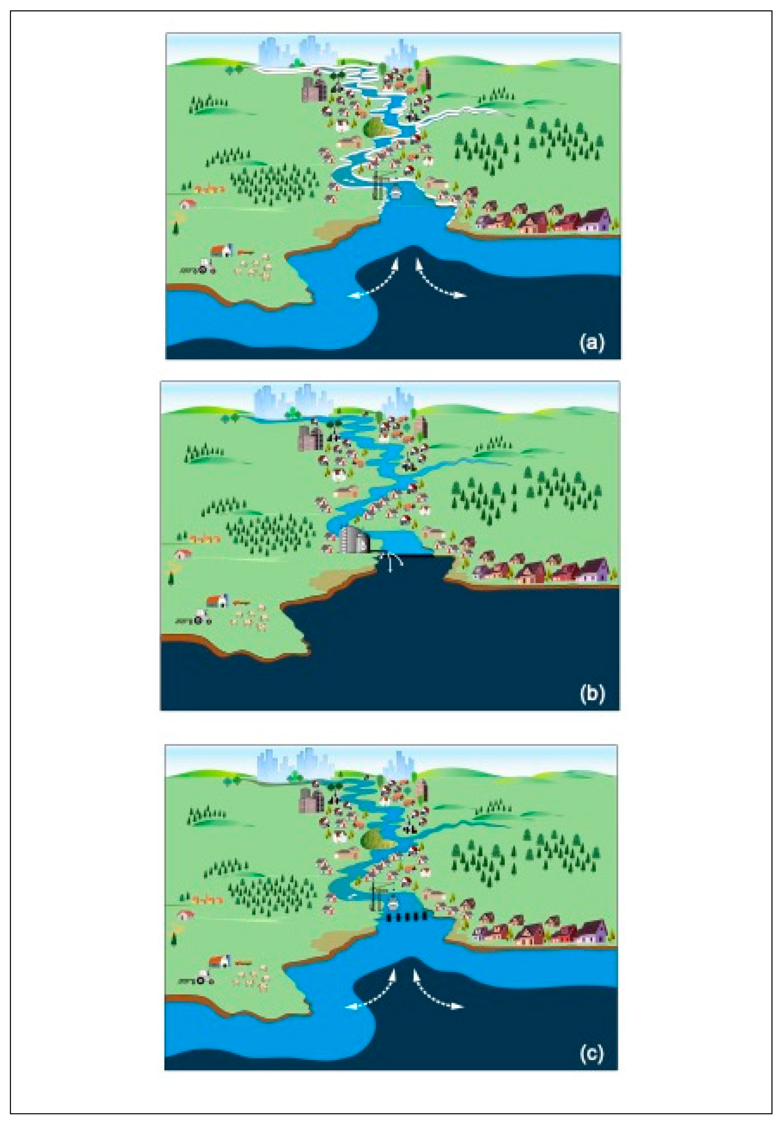
Figure 2.
(a) Map showing the location and (b) photo of the Eastern Scheldt Storm Surge Barrier, in the Netherlands (photo credit – Rijkswaterstaat). (c) Map showing the location and (b) photo of the Thames Storm Surge Barrier in the UK (photo credit – Ivan Haigh).
Figure 2.
(a) Map showing the location and (b) photo of the Eastern Scheldt Storm Surge Barrier, in the Netherlands (photo credit – Rijkswaterstaat). (c) Map showing the location and (b) photo of the Thames Storm Surge Barrier in the UK (photo credit – Ivan Haigh).

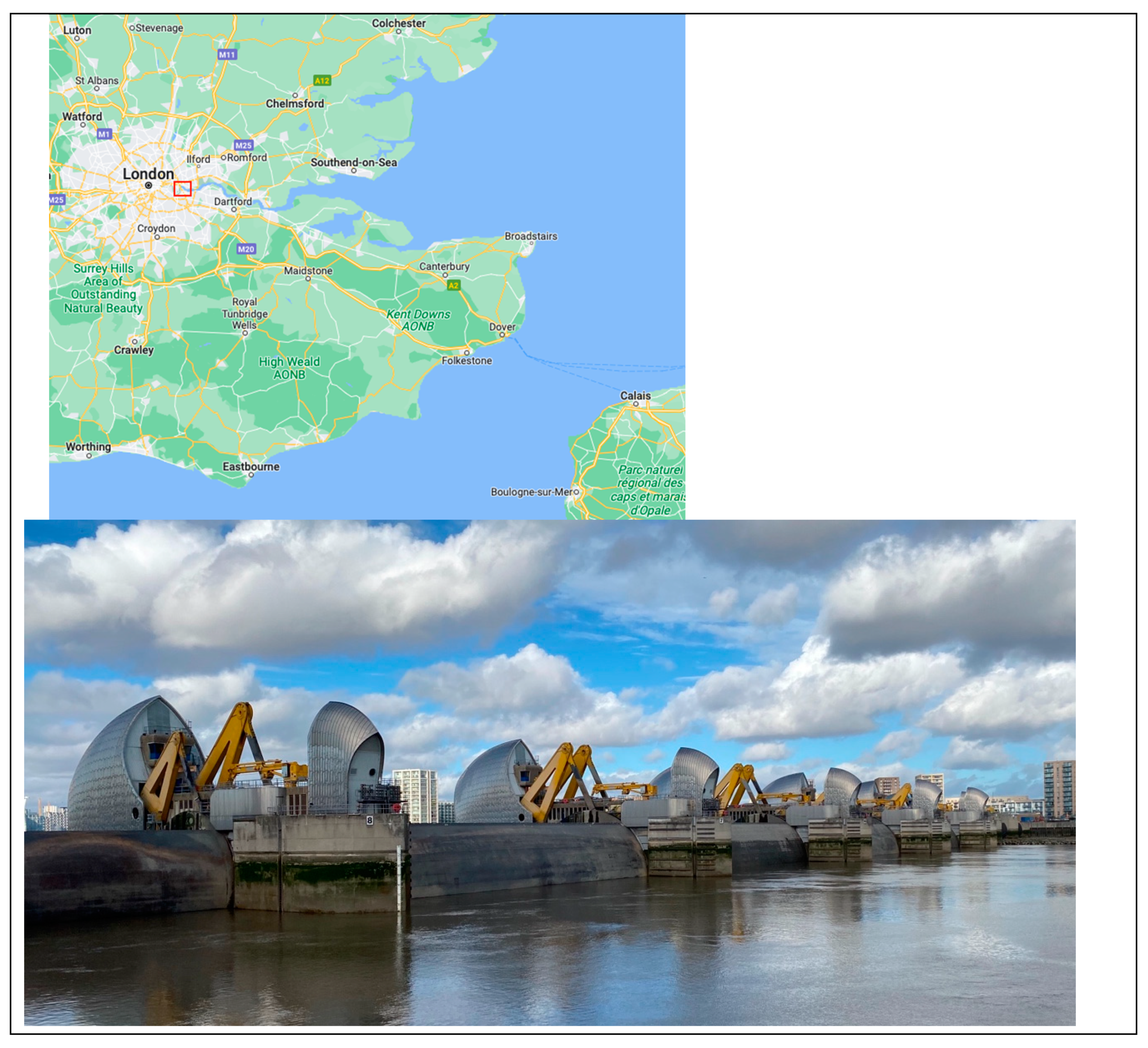
Figure 3.
(a) Total number of simulated and actual closures of the Eastern Scheldt Barrier from 1986/87 – 2023/24. (b) Total number of simulated and actual closures of the Thames Barrier from 1982/83 – 2023/24. (c) Mean number of simulated and actual closures per year of the Eastern Scheldt Barrier from 1986/87 – 2023/24. (d) Mean number of simulated and actual closures per year of the Thames Barrier from 1982/83 – 2023/24.
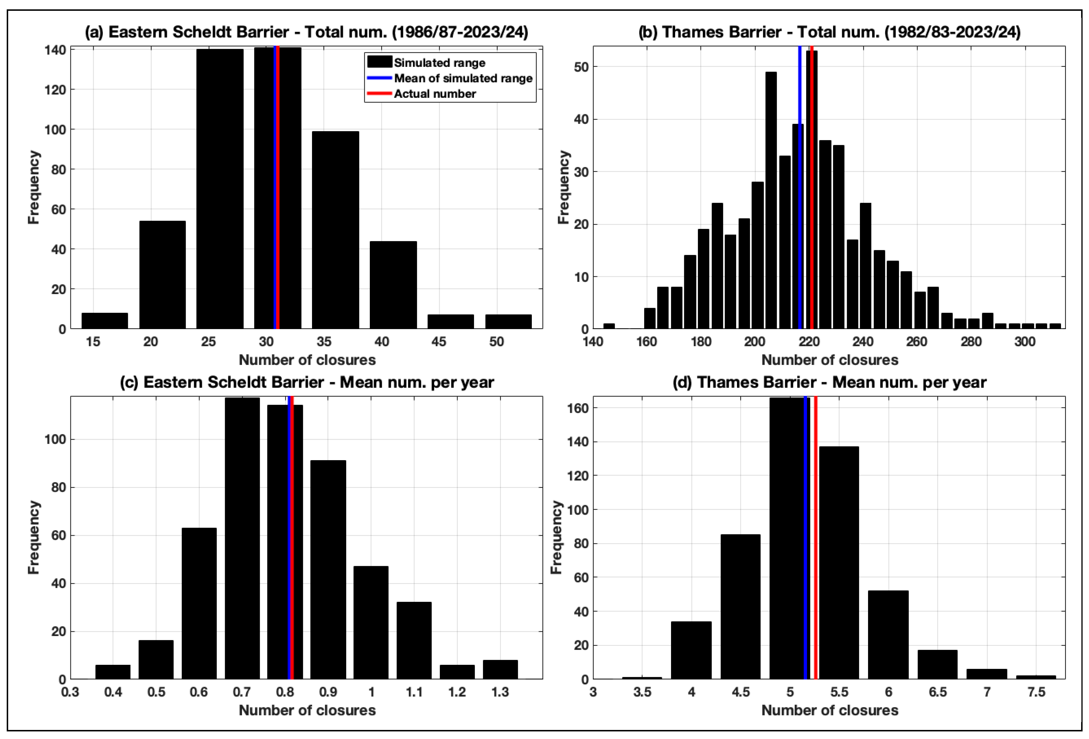
Figure 4.
Estimated number of barrier closures for four different sea level rise projections for the (a) Eastern Scheldt Barrier and (b) Thames Barrier and a water level forecast error of 0.2 m. Shown in (c) are the 4.4 year and 18.6 year inter-annual astronomical tidal cycles for Southend-on-Sea.
Figure 4.
Estimated number of barrier closures for four different sea level rise projections for the (a) Eastern Scheldt Barrier and (b) Thames Barrier and a water level forecast error of 0.2 m. Shown in (c) are the 4.4 year and 18.6 year inter-annual astronomical tidal cycles for Southend-on-Sea.
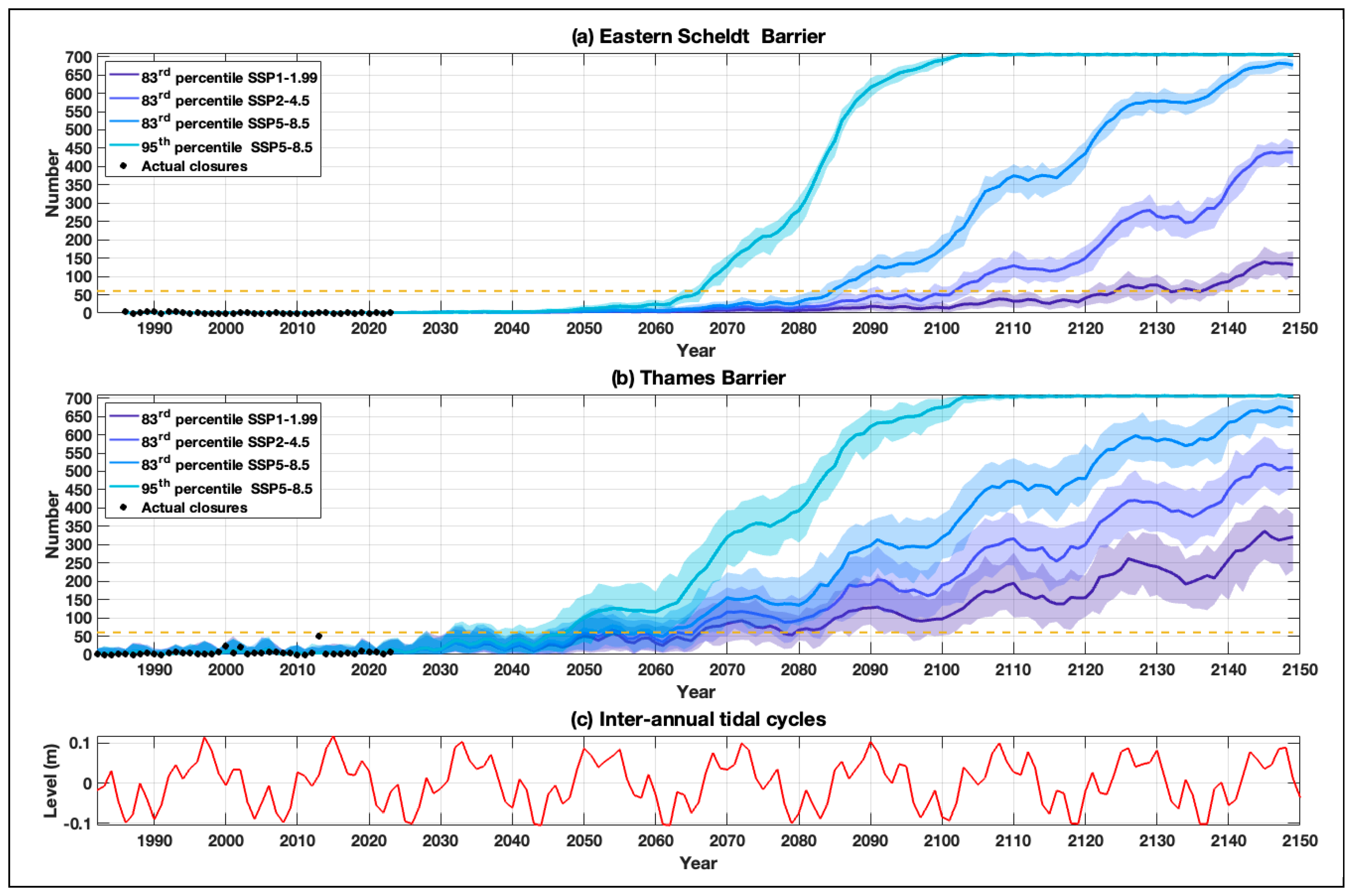
Figure 5.
The dates when barrier closures are recorded for the Thames Barrier for 1 of the 500 synthetic time-series, for four different sea level rise projections for the (a) low emission scenario; (b) medium emission scenario; (c) high emission scenario; and (d) high-end (e.g., low-likelihood but high impact) scenario.
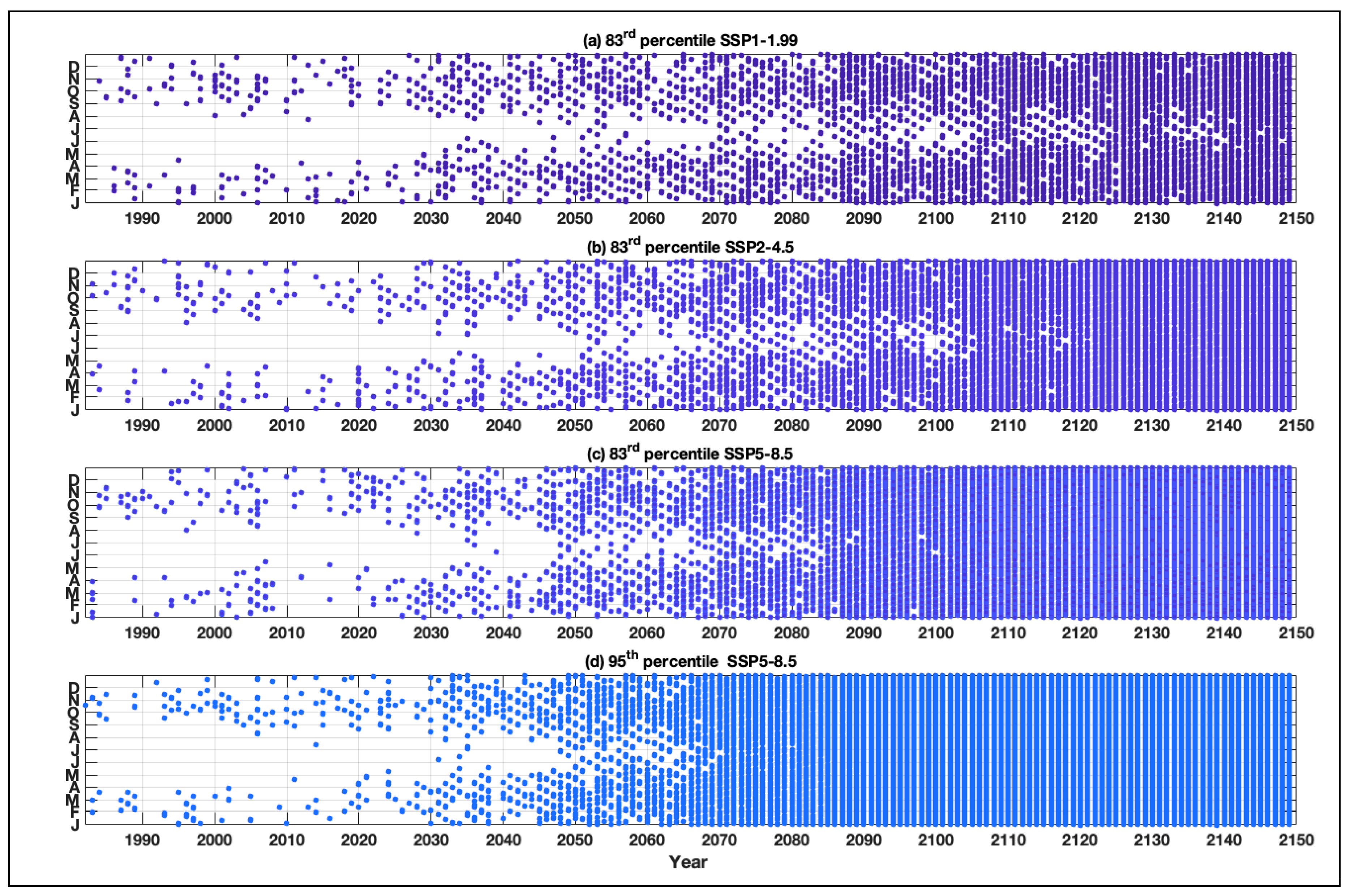
Figure 6.
Estimated number of barrier closures for four different projections of increases in skew surges for the (a) Eastern Scheldt Barrier and (b) Thames Barrier, for the IPCC AR6 SSP585 83rd percentile sea-level rise projection and a water level forecast error of 0.2 m. Shown in (c) are the 4.4 year and 18.6 year inter-annual astronomical tidal cycles for Southend-on-Sea.
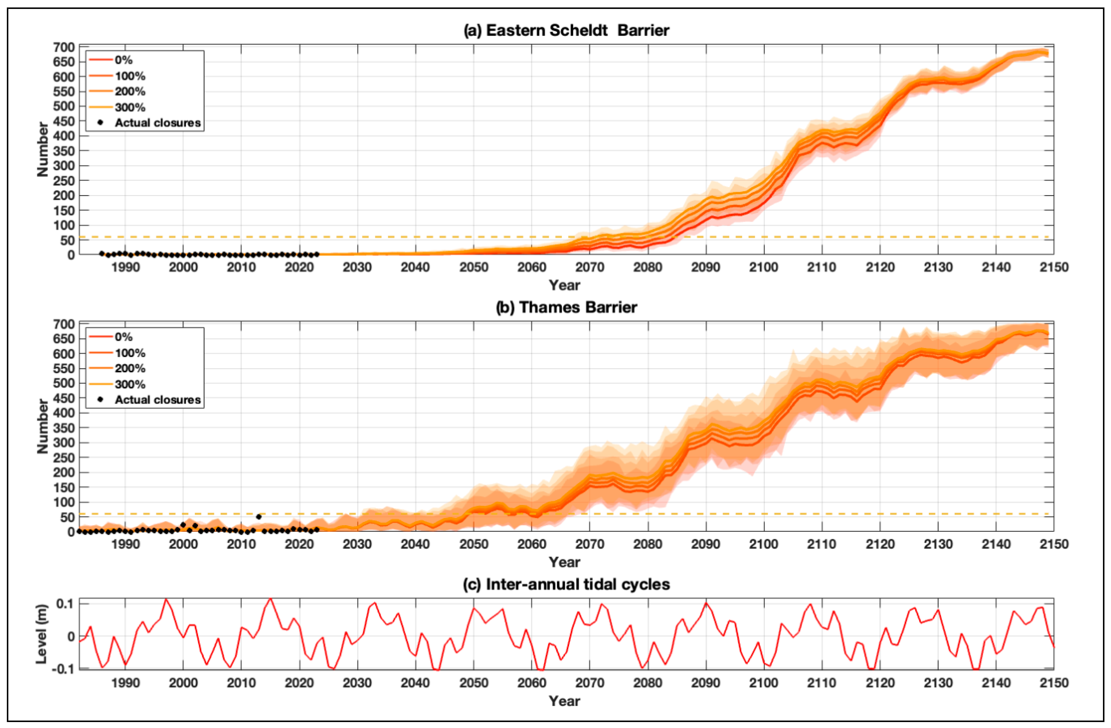
Figure 7.
Estimated number of barrier closures for four different projections of increases in tidal range for the (a) Eastern Scheldt Barrier and (b) Thames Barrier, for the IPCC AR6 SSP585 83rd percentile sea-level rise projection and a water level forecast error of 0.2 m. Shown in (c) are the 4.4 year and 18.6 year inter-annual astronomical tidal cycles for Southend-on-Sea.
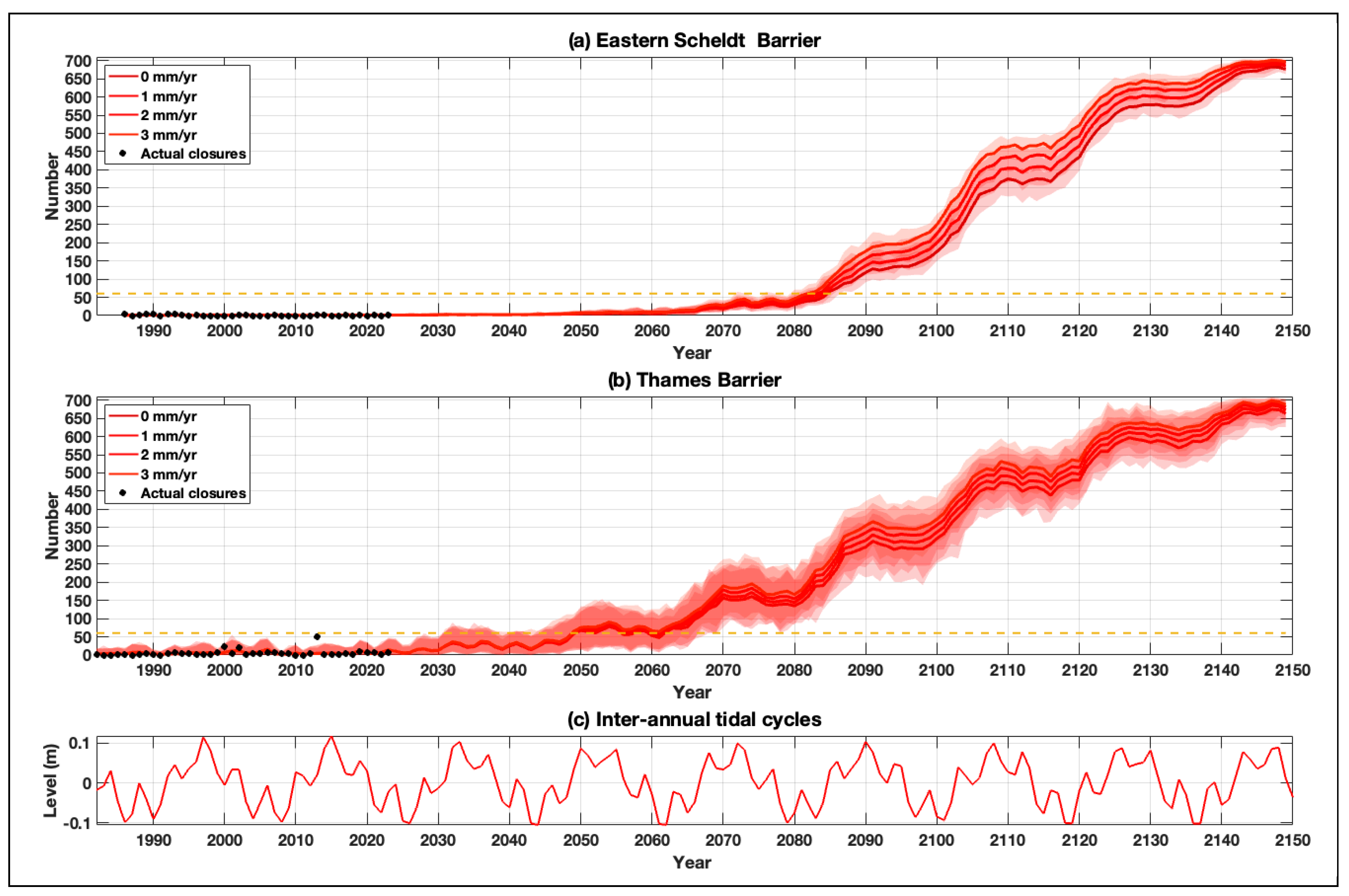
Figure 8.
(a) Estimated number of barrier closures for four different projections of increases in river discharge for the Thames Barrier, for the IPCC AR6 SSP585 83rd percentile sea-level rise projection and a water level forecast error of 0.2 m. Shown in (b) are the 4.4 year and 18.6 year inter-annual astronomical tidal cycles for Southend-on-Sea.
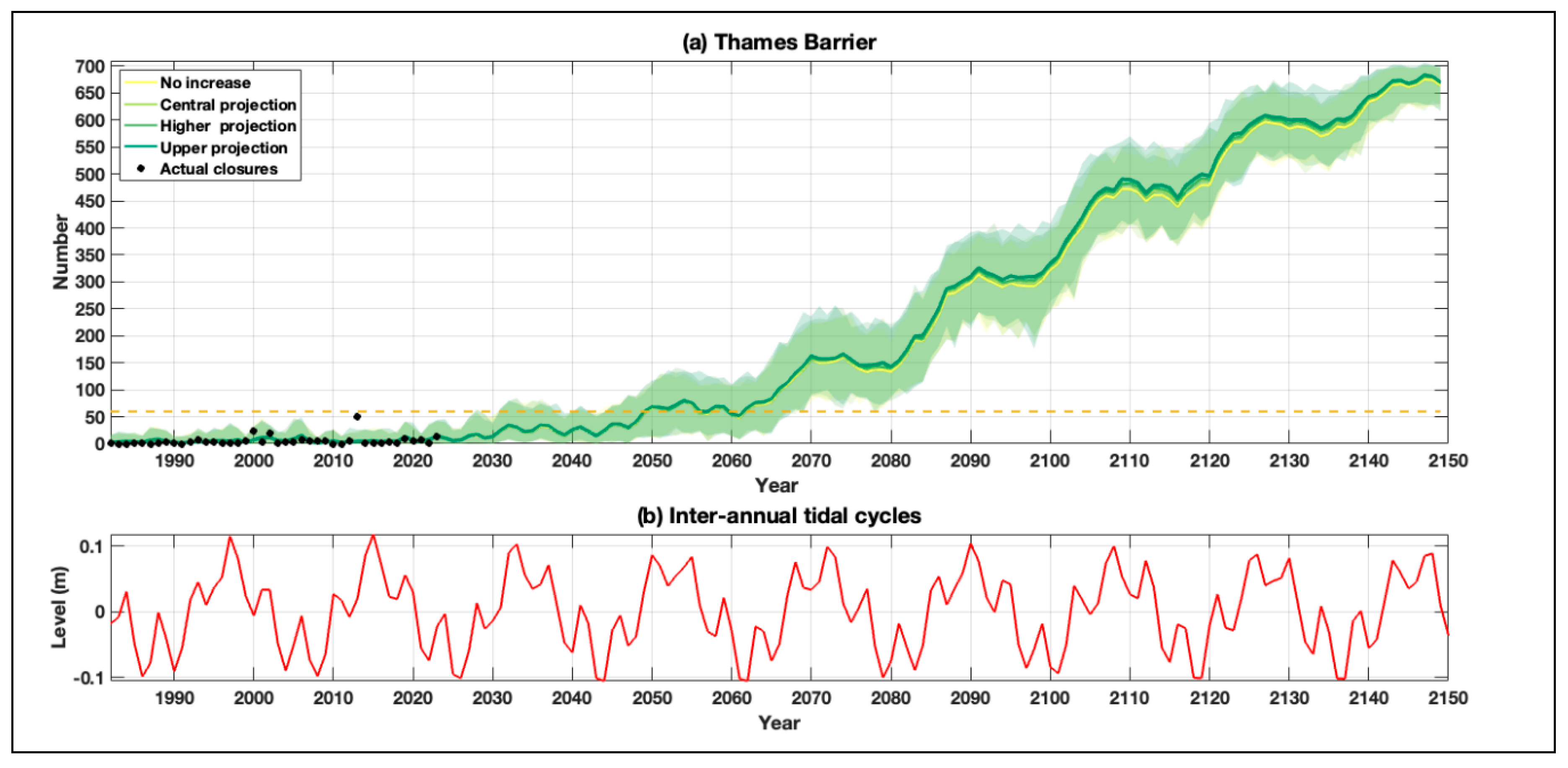
Figure 9.
Estimated number of barrier closures for four different forecast errors for the (a) Eastern Scheldt Barrier and (b) Thames Barrier, for the IPCC AR6 SSP585 83rd percentile sea-level rise projection and a water level forecast error of 0.2 m. Shown in (c) are the 4.4 year and 18.6 year inter-annual astronomical tidal cycles.

Figure 10.
Illustration of number of barrier closures for the Thames Barrier, considering an adaptative management pathway, corresponding with a planned 0.5 m raise in tidal defences upstream of the barrier, completed by 2050, with a planned further 0.5 m rise in tidal defences upstream of the barrier, completed by 2090, for the IPCC AR6 SSP585 83rd percentile sea-level rise projection and a water level forecast error of 0.2 m. .
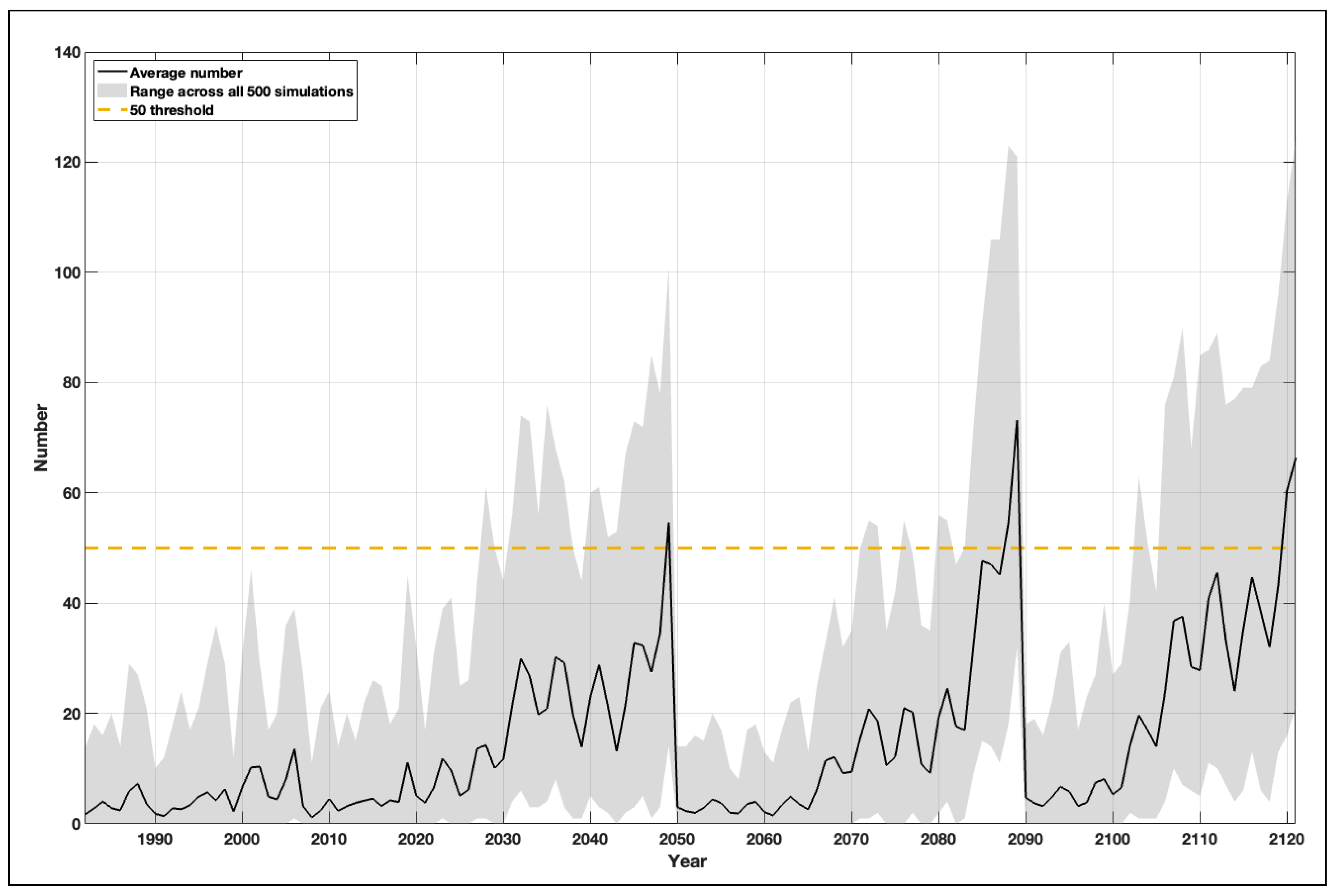

Table 1.
SLR projections, in meters relative to a 1995-2014 baseline, from the Intergovernmental Panel on Climate Change Sixth Assessment Report (Fox-Kemper et al., 2021) for the locations nearest to the Roompot Buiten and Southend tide gauge obtained from the NASA Sea Level Project Tool webpage (https://sealevel.nasa.gov/ipcc-ar6-sea-level-projection-tool).
| Scenario | Percentile | Confidence | 2020 | 2030 | 2040 | 2050 | 2060 | 2070 | 2080 | 2090 | 2100 | 2110 | 2120 | 2130 | 2140 | 2150 |
|---|---|---|---|---|---|---|---|---|---|---|---|---|---|---|---|---|
| Roompot Buiten – Eastern Scheldt | ||||||||||||||||
| SSP1-1.19 | 83 | medium | 0.132 | 0.206 | 0.264 | 0.330 | 0.397 | 0.477 | 0.545 | 0.600 | 0.662 | 0.738 | 0.810 | 0.879 | 0.949 | 1.018 |
| SSP2-4.5 | 83 | medium | 0.112 | 0.183 | 0.251 | 0.348 | 0.443 | 0.541 | 0.640 | 0.739 | 0.848 | 0.958 | 1.070 | 1.184 | 1.294 | 1.405 |
| SSP5-8.5 | 83 | medium | 0.110 | 0.178 | 0.263 | 0.379 | 0.495 | 0.621 | 0.760 | 0.922 | 1.119 | 1.277 | 1.450 | 1.618 | 1.783 | 1.945 |
| SSP5-8.5 | 95 | low | 0.139 | 0.229 | 0.365 | 0.540 | 0.733 | 0.976 | 1.290 | 1.681 | 2.133 | 2.607 | 3.157 | 3.790 | 4.561 | 5.742 |
| Southend – Thames Barrier | ||||||||||||||||
| SSP1-1.19 | 83 | medium | 0.142 | 0.216 | 0.273 | 0.342 | 0.415 | 0.496 | 0.563 | 0.618 | 0.68 | 0.757 | 0.831 | 0.902 | 0.973 | 1.043 |
| SSP2-4.5 | 83 | medium | 0.074 | 0.122 | 0.176 | 0.248 | 0.314 | 0.381 | 0.452 | 0.518 | 0.602 | 0.652 | 0.724 | 0.795 | 0.866 | 0.934 |
| SSP5-8.5 | 83 | medium | 0.109 | 0.181 | 0.27 | 0.381 | 0.495 | 0.623 | 0.766 | 0.928 | 1.12 | 1.278 | 1.45 | 1.62 | 1.785 | 1.946 |
| SSP5-8.5 | 95 | low | 0.137 | 0.232 | 0.37 | 0.543 | 0.732 | 0.977 | 1.294 | 1.683 | 2.138 | 2.6 | 3.155 | 3.789 | 4.576 | 5.766 |
Table 2.
The average number of closures per year, averaged over each decade from 1990-2000 to 2140-2150, for the 4 SLR scenarios (the 83rd percentile of projection SSP1-1.99, which equates to a low emission scenario; the 83rd percentile of projection SSP2-4.5, which equates to a medium emission scenario; the 83rd percentile of projection SSP5-8.5, which equates to a high emission scenario; ad the 95th percentile of the low confidence projection SSP5-8.5, which equates to a high-end, e.g., low-likelihood but high impact, scenario). We ran these simulations with a water level forecast error of 0.2 m for both barriers.
| Decade | Eastern Scheldt Barrier | Thames Barrier | ||||||
|---|---|---|---|---|---|---|---|---|
| 83rd SSP1-1.99 | 83rd SSP2-4.5 | 83rd SSP5-8.5 | 95th SSP5- 8.5 | 83rd SSP1-1.99 | 83rd SSP2-4.5 | 83rd SSP5-8.5 | 95th SSP5- 8.5 | |
| 1980-1989 | 1.2 | 1.1 | 1.2 | 1.2 | 4.4 | 4.5 | 4.4 | 4.4 |
| 1990-1999 | 1.1 | 1.1 | 1.1 | 1.1 | 4.0 | 3.9 | 4.0 | 4.0 |
| 2000-2009 | 1.1 | 1.1 | 1.1 | 1.1 | 7.4 | 7.3 | 7.5 | 7.3 |
| 2010-2019 | 1.2 | 1.2 | 1.2 | 1.1 | 5.1 | 5.2 | 5.1 | 5.2 |
| 2020-2029 | 1.4 | 1.4 | 1.4 | 1.4 | 10 | 10 | 10 | 10 |
| 2030-2039 | 2.2 | 2.2 | 2.3 | 2.8 | 23 | 23 | 25 | 31 |
| 2040-2049 | 2.5 | 2.7 | 3.1 | 5.3 | 24 | 26 | 31 | 49 |
| 2050-2059 | 4.0 | 5.2 | 6.6 | 17 | 45 | 55 | 66 | 118 |
| 2060-2069 | 5.3 | 8 | 12 | 55 | 50 | 66 | 86 | 190 |
| 2070-2079 | 8 | 14 | 25 | 197 | 76 | 106 | 147 | 353 |
| 2080-2089 | 11 | 26 | 63 | 451 | 93 | 140 | 212 | 508 |
| 2090-2099 | 16 | 44 | 135 | 654 | 108 | 180 | 298 | 646 |
| 2100-2109 | 26 | 87 | 277 | 702 | 146 | 255 | 406 | 697 |
| 2110-2119 | 32 | 124 | 381 | 706 | 157 | 285 | 461 | 705 |
| 2120-2129 | 61 | 228 | 530 | 706 | 222 | 383 | 560 | 706 |
| 2130-2139 | 68 | 269 | 586 | 706 | 216 | 397 | 586 | 706 |
| 2140-2149 | 122 | 411 | 667 | 706 | 305 | 496 | 659 | 706 |
Table 3.
The average number of closures per year, averaged over each decade from 1990-2000 to 2140-2150, for the 4 skew surge scenarios (0, 100, 200 and 300% increase in skew surges by 2150). We ran these simulations with the high emission SLR scenario (83rd percentile of projection SSP5-8.5) and a water level forecast error of 0.2 m for both barriers.
| Decade | Eastern Scheldt Barrier | Thames Barrier | ||||||
|---|---|---|---|---|---|---|---|---|
| 0% | 100% | 200% | 300% | 0% | 100% | 200% | 300% | |
| 1980-1989 | 1.2 | 1.2 | 1.2 | 1.2 | 4.4 | 4.4 | 4.4 | 4.4 |
| 1990-1999 | 1.1 | 1.1 | 1.1 | 1.1 | 4.0 | 4.0 | 3.9 | 4.0 |
| 2000-2009 | 1.1 | 1.1 | 1.1 | 1.1 | 7.5 | 7.4 | 7.3 | 7.5 |
| 2010-2019 | 1.2 | 1.2 | 1.2 | 1.2 | 5.1 | 5.1 | 5.1 | 5.3 |
| 2020-2029 | 1.4 | 1.5 | 1.5 | 1.6 | 10 | 10 | 10 | 10 |
| 2030-2039 | 2.3 | 2.7 | 3.2 | 3.7 | 25 | 26 | 27 | 29 |
| 2040-2049 | 3.1 | 4.4 | 5.8 | 7.5 | 31 | 34 | 37 | 39 |
| 2050-2059 | 6.6 | 10 | 14 | 18 | 66 | 72 | 79 | 84 |
| 20602069 | 12 | 18 | 26 | 34 | 86 | 95 | 104 | 113 |
| 2070-2079 | 25 | 38 | 52 | 65 | 147 | 161 | 173 | 187 |
| 2080-2089 | 63 | 82 | 102 | 120 | 212 | 228 | 244 | 259 |
| 2090-2099 | 135 | 163 | 187 | 205 | 298 | 318 | 335 | 349 |
| 2100-2109 | 277 | 303 | 321 | 336 | 406 | 425 | 440 | 451 |
| 2110-2119 | 381 | 402 | 416 | 427 | 461 | 479 | 492 | 504 |
| 2120-2129 | 529 | 542 | 548 | 553 | 560 | 573 | 581 | 587 |
| 2130-2139 | 586 | 595 | 598 | 600 | 586 | 598 | 605 | 609 |
| 2140-2149 | 667 | 669 | 669 | 669 | 659 | 663 | 664 | 666 |
Table 4.
The average number of closures per year, averaged over each decade from 1990-2000 to 2140-2150, for the 4 tidal range scenarios (0, 1, 2 and 3 mm/yr increase in tidal range). We ran these simulations with the high emission SLR scenario (83rd percentile of projection SSP5-8.5) and a water level forecast error of 0.2 m for both barriers.
| Decade | Eastern Scheldt Barrier | Thames Barrier | ||||||
|---|---|---|---|---|---|---|---|---|
| 0 mm/yr | 1 mm/yr | 2 mm/yr | 3 mm/yr | 0 mm/yr | 1 mm/yr | 2 mm/yr | 3 mm/yr | |
| 1980-1989 | 1.2 | 1.2 | 1.1 | 1.2 | 4.4 | 4.4 | 4.4 | 4.4 |
| 1990-1999 | 1.1 | 1.1 | 1.1 | 1.1 | 4.0 | 4.0 | 4.0 | 4.0 |
| 2000-2009 | 1.1 | 1.1 | 1.1 | 1.1 | 7.5 | 7.4 | 7.5 | 7.4 |
| 2010-2019 | 1.2 | 1.2 | 1.1 | 1.2 | 5.1 | 5.1 | 5.2 | 5.2 |
| 2020-2029 | 1.4 | 1.4 | 1.4 | 1.4 | 10 | 10 | 10 | 10 |
| 2030-2039 | 2.3 | 2.3 | 2.4 | 2.5 | 25 | 25 | 26 | 27 |
| 2040-2049 | 3.1 | 3.3 | 3.5 | 3.7 | 31 | 33 | 34 | 36 |
| 2050-2059 | 6.6 | 7.1 | 7.9 | 8.5 | 66 | 70 | 74 | 78 |
| 20602069 | 12 | 13 | 15 | 17 | 86 | 92 | 98 | 106 |
| 2070-2079 | 25 | 29 | 34 | 39 | 147 | 157 | 169 | 180 |
| 2080-2089 | 63 | 73 | 85 | 98 | 212 | 227 | 242 | 257 |
| 2090-2099 | 135 | 156 | 177 | 201 | 298 | 316 | 335 | 353 |
| 2100-2109 | 277 | 308 | 339 | 370 | 406 | 425 | 444 | 461 |
| 2110-2119 | 381 | 413 | 444 | 473 | 461 | 480 | 498 | 515 |
| 2120-2129 | 530 | 557 | 581 | 603 | 560 | 577 | 593 | 608 |
| 2130-2139 | 586 | 608 | 628 | 645 | 586 | 603 | 619 | 632 |
| 2140-2149 | 667 | 678 | 687 | 693 | 659 | 670 | 679 | 686 |
Table 5.
The average number of closures per year, averaged over each decade from 1990-2000 to 2140-2150, for the 4 river discharge scenarios (no change, central, higher and upper projection). Note, results are only listed for the Thames Barrier, as river discharge does not determine closure thresholds at the Eastern Scheldt Barrier. We ran these simulations with the high emission SLR scenario (83rd percentile of projection SSP5-8.5) and a water level forecast error of 0.2 m.
| Decade | Thames Barrier | |||
|---|---|---|---|---|
| No change | Central | Higher | Upper | |
| 1980-1989 | 4.4 | 4.5 | 4.4 | 4.4 |
| 1990-1999 | 4.0 | 3.9 | 4.0 | 4.0 |
| 2000-2009 | 7.5 | 7.4 | 7.5 | 7.3 |
| 2010-2019 | 5.1 | 5.2 | 5.2 | 5.2 |
| 2020-2029 | 10 | 10 | 10 | 10 |
| 2030-2039 | 25 | 25 | 25 | 26 |
| 2040-2049 | 31 | 31 | 32 | 32 |
| 2050-2059 | 66 | 67 | 67 | 68 |
| 20602069 | 86 | 87 | 88 | 90 |
| 2070-2079 | 147 | 149 | 150 | 154 |
| 2080-2089 | 212 | 216 | 218 | 222 |
| 2090-2099 | 298 | 303 | 306 | 312 |
| 2100-2109 | 406 | 413 | 415 | 422 |
| 2110-2119 | 461 | 470 | 471 | 479 |
| 2120-2129 | 560 | 567 | 568 | 574 |
| 2130-2139 | 586 | 594 | 595 | 601 |
| 2140-2149 | 659 | 663 | 664 | 667 |
Table 6.
The average number of closures per year, averaged over each decade from 1990-2000 to 2140-2150, for the 4 forecast water level scenarios (0, 0.1, 0.2 and 0.3 m forecast errors). We ran these simulations with the high emission SLR scenario (83rd percentile of projection SSP5-8.5) and a water level forecast error of 0.2 m for both barriers.
| Decade | Eastern Scheldt Barrier | Thames Barrier | ||||||
|---|---|---|---|---|---|---|---|---|
| 0 m | 0.1 m | 0.2 m | 0.3 m | 0 m | 0.1 m | 0.2 m | 0.3 m | |
| 1980-1989 | 0.5 | 0.7 | 1.2 | 1.9 | 1.1 | 2.2 | 4.4 | 8.5 |
| 1990-1999 | 0.4 | 0.7 | 1.1 | 1.8 | 1.0 | 2.0 | 4.0 | 8.1 |
| 2000-2009 | 0.5 | 0.7 | 1.1 | 1.7 | 2.0 | 4.0 | 7.4 | 13.5 |
| 2010-2019 | 0.5 | 0.8 | 1.1 | 1.8 | 1.4 | 2.7 | 5 | 10 |
| 2020-2029 | 0.6 | 0.9 | 1.4 | 2.2 | 2.5 | 4.9 | 10 | 18 |
| 2030-2039 | 0.9 | 1.5 | 2.3 | 3.8 | 7.2 | 13.5 | 25 | 42 |
| 2040-2049 | 1.2 | 1.9 | 3.1 | 5 | 10 | 19 | 31 | 49 |
| 2050-2059 | 2.4 | 3.9 | 6.7 | 12 | 26 | 43 | 66 | 96 |
| 20602069 | 4.1 | 7 | 12 | 21 | 39 | 59 | 86 | 119 |
| 2070-2079 | 8 | 15 | 26 | 45 | 75 | 108 | 147 | 193 |
| 2080-2089 | 20 | 36 | 63 | 103 | 126 | 166 | 212 | 262 |
| 2090-2099 | 52 | 86 | 135 | 200 | 194 | 244 | 298 | 352 |
| 2100-2109 | 137 | 202 | 277 | 357 | 303 | 355 | 407 | 455 |
| 2110-2119 | 222 | 300 | 381 | 455 | 362 | 413 | 461 | 505 |
| 2120-2129 | 394 | 466 | 530 | 584 | 479 | 521 | 560 | 594 |
| 2130-2139 | 474 | 535 | 586 | 627 | 513 | 551 | 587 | 618 |
| 2140-2149 | 602 | 640 | 667 | 685 | 609 | 637 | 659 | 676 |
Disclaimer/Publisher’s Note: The statements, opinions and data contained in all publications are solely those of the individual author(s) and contributor(s) and not of MDPI and/or the editor(s). MDPI and/or the editor(s) disclaim responsibility for any injury to people or property resulting from any ideas, methods, instructions or products referred to in the content. |
© 2024 by the authors. Licensee MDPI, Basel, Switzerland. This article is an open access article distributed under the terms and conditions of the Creative Commons Attribution (CC BY) license (http://creativecommons.org/licenses/by/4.0/).
Copyright: This open access article is published under a Creative Commons CC BY 4.0 license, which permit the free download, distribution, and reuse, provided that the author and preprint are cited in any reuse.


