
Submitted:
27 October 2024
Posted:
28 October 2024
You are already at the latest version
Abstract
Low-cost sensors are widely used for air quality monitoring due to their affordability, portability and easy maintenance. However, the performance of such sensors, such as PurpleAir Sensors (PAS), is often affected by changes in environmental (e.g., temperature and humidity) or emission conditions, and hence the resulting measurements require corrections to ensure accuracy and validity. Traditional correction methods, like those developed by the US-EPA, have limitations, particularly for applications to geographically diverse settings and sensors with no collocated referenced monitoring stations available. This study introduces BaySurcls, a Bayesian-optimised surrogate model integrating deep learning (DL) algorithms to improve the PurpleAir sensors PM2.5 (PAS2.5) measurement accuracy. The framework incorporates environmental variables such as humidity and temperature alongside aerosol characteristics, to refine sensor readings. The BaySurcls model corrects the PAS2.5 data for both collocated and non-collocated monitoring scenarios. A case study showed that BaySurcls outperforms all tested standalone models (DL or classical machine learning based) and the US-EPA correction method in terms of reducing root mean square errors in PAS2.5 data and enhancing correlations with the reference data, under both the collocation and non-collocation monitoring scenarios. This improvement is evident across multiple locations in New South Wales, Australia, demonstrating the model's adaptability. The findings confirm BaySurcls as a promising solution for improving the reliability of low-cost sensor data, thus facilitating its valid use in air quality research, impact assessment, and environmental management.
Keywords:
Machine Learning (ML)
; Deep Learning (DL)
; BaySurcls
; PurpleAir Sensor (PAS)
; PM2.5 Pollution
; Data Correction
1. Introduction
Air pollution is a significant global environmental hazard, adversely affecting human health and ecosystems [1,2]. PM2.5, particulate matter (PM) with an aerodynamic diameter of less than 2.5 µm, is regarded as the most detrimental air pollutant species to health, resulting in more morbidities and mortalities than any other pollutant [3,4,5,6,7]. Substantial health repercussions are discernible even at low PM2.5 concentrations [8] – studies showed that a small increment (as low as 1-10 µg/m3) can have adverse effects on human health [7,8,9,10,11]. Therefore, measuring and comprehending PM2.5 pollution can help counter the potentially damaging effect and mitigate risks to human health and the environment.
Typically, regulatory authorities install a limited number of conventional/compliance (often standards-based) air quality stations at strategic locations to monitor, evaluate and inform local and regional population exposure to air pollution, primarily due to resourcing constraints including site accessibility, installation cost and labour-intensive maintenance demand. However, (spatially and temporally) enhanced monitoring is often required to better inform and prepare citizens for minimising their exposure to air pollution (including PM2.5), since pollutant concentrations often display considerable spatial and temporal variability influenced by characteristics of the natural and built environments and emission sources [12,13,14].
In recent years, there has been a notable rise in the application of low-cost sensing technologies for PM2.5 monitoring, being significant supplement to the compliance PM2.5 monitoring networks. This is in part attributed to the diminished (low) cost, higher portability, low-power demand and compact dimensions of low-cost sensors (LCSs) [15,16,17,18,19]. Broadly, for example, PurpleAir sensor (PAS) is becoming prevalent and extensively employed by individuals, community organizations, and air monitoring agencies, constituting a massive worldwide network of over 10,000 sensors [10,20]. More locally, the New South Wales (NSW) government has been exploring the utility of LCSs in the state, a subtropical environment in the Southern Hemisphere. In recent years, over a hundred PASs have been deployed within different airsheds across NSW, primarily including two types of installations: 1) sensors collocated at some individual compliance (reference) air monitoring stations (referred to as ‘ “collocation monitoring scenario” in this text) to allow for data calibration/comparison; and 2) those (majority) installed through voluntary citizens and located in areas where there are no government operated (reference) stations (referred to as “non-collocation monitoring scenario” in this text).
Nonetheless, it is known that raw PAS data can exhibit considerable biases because the sensors are sensitive to meteorological conditions, such as temperature and relative humidity [21,22], and pollutant cross-sensitivities [14,23,24,25]. Prior research has examined the precision and efficacy of PASs in laboratories [26] and fields in various countries including the United States [27,28,29,30,31,32,33,34,35], Australia [3], Korea [36], Greece [37], Sri Lanka [38], and Uganda [39]. Numerous investigations indicate that the PAS generates a consistent normalized particle size distribution, irrespective of the actual size distribution and concentration. Barkjohn, Gantt and Clements [10] found that the raw data from PASs overstated PM2.5 concentrations by around 40% in most of the United States under typical ambient and smoke-impacted conditions. Therefore, PAS measurements must be corrected to provide PM2.5 data compatible to those from regulatory monitors, prior to its use for air quality reporting or research. Currently, correcting PASs at typical ambient pollutant concentrations and environmental conditions remains a primary challenge.
Several previous statistical correction methods have been developed for PAS data. For example, the United States Environmental Protection Agency (EPA) formulated correction equations (for nationwide applications) that consider effects of relative humidity on PAS measurement accuracy [10]. Further, Jaffe, Thompson, Finley, Nelson, Ouimette and Andrews [20] proposed and evaluated a new EPA correction algorithm, which yielded satisfactory PM2.5 data for typical urban wintertime pollution and smoke occurrences but underestimated PM2.5 during dust events by a factor of 5-6. These traditional empirical correction methods are usually tailored to a particular location, season, or circumstance. Recently, there has been some growing interest in applying machine learning (ML) approaches for PAS data correction. Chojer, et al. [40] compared Multiple Linear Regression (MLR), Support Vector Regression (SVR), Gradient Boosting Regression (GBR) and Extreme Gradient Boosting (XGB), concluding that the in-field calibration method yielded good accuracy with the boosting and SVR models. Yu, et al. [41] applied Automated Machine Learning-Land Use Regression (AutoML-LUR) and discovered that integrating PAS data into the model enhances predictive performance, especially in regions with few regulatory monitoring stations. Kar, et al. [42] used Random Forest (RF)[42], Random Forest Spatial Interpolation (RFSI), Space-Time Regression Kriging (STRK) and Random Forest Kriging (RFK), and they found that STRK outperformed other ML models. While these approaches may enhance the dependability/utility/validity of PAS PM2.5 data, the training of ML-based correction models generally requires sufficient observational data from collocated (standard) reference monitors. To address this issue, we expect transfer learning, which utilises knowledge (or model) obtained from abundant data derived from a limited array of sensors and/or monitors, enhances the model for the target task and reduces the reliance on reference monitors.
In this study, we propose a Bayesian-optimised deep-learning (DL)-based surrogate model (framework) for improving the accuracy of PM2.5 data obtained under both the collocation and non-collocation PurpleAir sensors monitoring scenarios in NSW (details in Section 2). The study is focused on comparing the efficacy of the proposed framework with a few commonly used standalone DL models and the well-established US-EPA PAS data correction method, to determine which approach yields more accurate and dependable PM2.5 data. The study aims to deliver more accurate LCS data for air quality research and reporting. The findings will form the foundation of further work on data fusion, impact assessment and air quality nowcasting and forecasting in NSW. The results and approach can also be useful for other jurisdictions in Australia, or similar regions elsewhere.
2. Data and Method
2.1. Study Area and Monitoring Sites
This study focuses on New South Wales (NSW), which has a population exceeding 8 million in an area of approximately 801,150 km2. Air pollution remains an issue in NSW, and exposure to PM, even at minimal concentrations, has been shown to elevate hospital admissions for cardiovascular disease outcomes among the elderly in Sydney [43,44]. It is reported that over 50% of (primary) PM2.5 emissions stem from household and commercial sources in NSW, with secondary particles also formed in the atmosphere through complex chemical reactions from precursor pollutants such as nitrogen oxides, sulfur dioxides and ammonia [43,45,46].
The NSW Department of Climate Change, Energy, the Environment and Water (DCCEEW) manages a comprehensive network of air quality monitoring stations (AQMS) throughout NSW (https://www.airquality.nsw.gov.au/). As noted earlier, over a hundred PASs have been deployed within different airsheds across NSW, including sensors collocated at some compliance (reference) air monitoring stations so that direct comparison or correction can be made to improve the accuracy of PAS data, and those (majority) installed through voluntary citizens and located in areas where there are no government operated stations.
In our case study, we chose a total of 12 PASs across seven AQMS in NSW - Armidale, Merriwa, Millthorpe, Lidcombe, Newcastle, Bathurst, and Wagga-wagga-north (Figure 1; Table 1), to explore the utility of ML/DL in developing methods for improving the accuracy of PAS data. At these selected stations, each AQMS and its collocated PAS(s) have PM2.5 measurements available for relatively longer time (than other locations). These stations fall within six different air quality monitoring stations that exhibit varying land types, climatic conditions, pollutant levels and pollutant sources, including vehicle emissions, sea aerosols, and urban background pollutants.
2.2. Reference Data - Air Quality Monitoring Station PM2.5 Measuremets
The reference data for this study was sourced from seven (compliance) AQMS in the NSW Air Quality Monitoring Network for the same periods as the PAS data (details in 2.3), i.e., in slightly varying periods between 01/03/2020 and 30/7/2024 (Table 1, Figure 1). This included hourly PM2.5 measurements to benchmark the accuracy of raw PAS data and those corrected using BaySurcls and other methods. This diverse selection of station locations ensures that the AQMS data used as the reference point captured a wide array of environmental and air quality dynamics, essential for validating the accuracy of the corrected PAS data.
2.3. PurpleAir Sensor Data – PAS Measurements
Historical data for 12 PASs were obtained for slightly varying periods between 01/03/2020 and 30/7/2024 (Table 1), including 10 min readings for humidity, temperature, PAS2.5, CAF (Coarse Aerosol Fraction), MR (mass ratio), and PCR (Particle Count Ratio). The data were averaged to obtain hourly values. These variables, treated as predictors for the data correction models, combine to capture different aspects of the environmental and particle characteristics that influence how well the sensor performs, especially in varying atmospheric conditions and aerosol types [47].
Humidity can significantly affect the readings from PurpleAir sensors [48]. When humidity levels are high, particulate matter tends to absorb moisture, making particles appear larger than they are - this can cause overestimation of PM2.5 levels in raw sensor data. Barkjohn et al. [47] showed that an additive humidity correction model could improve PAS PM2.5 measurements using linear regression. By including humidity in the proposed correction algorithm, we can account for this moisture effect and potentially provide a more accurate measurement.
Although temperature does not directly impact particle size, it can influence the performance of sensor measuring particle concentrations and internal/ambient environmental conditions [49,50]. Inclusion of temperature helps to enable the correction algorithm to adjust for sensor performance in varying temperature environments, ensuring consistent performance across different climate zones.
PAS2.5 (ambient) is the core measurement from the PurpleAir sensor, representing the raw PM2.5 concentration. Coarse Aerosol Fraction (CAF) represents the fraction of coarse particles (PM10) relative to smaller particles (PM2.5), which helps differentiate between aerosol types. For example, dust events have a higher CAF, indicating a greater proportion of larger particles. Since PurpleAir sensors tend to underestimate PM2.5 during dust events [20], the CAF allows the correction algorithm to better adjust for such conditions. Moreover, the mass ratio (MR) between PM1 and PM10 provides insights into the size distribution of particles. A higher MR indicates a greater concentration of smaller particles (PM1), which is typical in urban pollution or smoke, whereas a lower ratio is seen in dust-dominated environments. Particle Count Ratio (PCR) ratio is used to further characterize the size distribution of particles, particularly in relation to dust aerosols. Table 2 provides relevant information of three rations. Dust events tend to have a lower PCR due to the dominance of larger particles, and this ratio has been used to identify when a more substantial correction is needed for PurpleAir sensors. By incorporating these variables as predictors in the correction algorithm, we address the key factors that contribute to sensor inaccuracies, particularly in different environmental contexts. We consider these inputs allow us to refine the PurpleAir PM2.5 readings for better integration into air quality models, which is especially important for applications in AI and predictive analytics.
In ideal situations, PAS readings are expected to be close to the AQMS (reference) data, i.e., the ratio for non-zero readings should be close to one. Figure 2 shows the boxplots of PM2.5 reading ratios for each AQMS-PAS pair. There are large amounts of data points with ratios greater than two across all AQMSs. In other words, there exist clear discrepancies between collocated AQMS and PAS readings. This highlights the need for correcting the PAS data prior to its valid use in air quality reporting and research.
2.4. Modelling Framework
As noted earlier, this study was focused on exploring the utility of the ML method for correcting PM2.5 measurements from PurpleAir sensors (i.e., PAS2.5) across NSW. A surrogate modelling framework, referred to as BaySurcls, was featured with a combination of five Bayesian-optimised DL architectures—Long Short-Term Memory (LSTM), Gated Recurrent Unit (GRU), Convolutional Neural Networks with LSTM (CNN-LSTM), CNN with GRU (CNN-GRU), and CNN with Bidirectional LSTM (CNN-BiLSTM) (Figure 3). These architectures are known for their ability to handle sequential and time-series data. The theoretical details of the algorithms are documented in the literature by various authors [51,52,53,54,55,56] and therefore are not repeated in this text. Hence, the hybrid BaySurcls is expected to capture the complex temporal and spatial dependencies inherent in air quality data, thus potentially could be applicable across different airsheds in the state.
To facilitate the model performance analysis, we used the standalone counterpart DL models (i.e., LSTM, GRU, CNN-GRU and CNN-LSTM) applied in the BaySurcls and a few classical machine learning models, Multiple Linear Regression (MLR), Random Forest (RF) and Support Vector Regression (SVR), as benchmark models. The comprehensive evaluation against the PAS2.5 data allowed us to understand how these models perform individually compared to our proposed hybrid model.
The proposed model is further evaluated (compared) with the US-EPA PurpleAir sensor data correction method, which serves as a baseline for improving the accuracy of PAS2.5 measurements. The US-EPA correction is an established approach, extensively used in both (formal) air quality reporting and research domains to align PurpleAir sensor measurements with reference-grade monitoring data. By comparing the correction of PAS2.5 using US-EPA method, we can ensure that the PAS2.5 data we used in our study met a level of accuracy that facilitates meaningful analysis and comparison. The use of such well-validated correction methods against the proposed/tested BaySurcls model and associated benchmark models helps to elevate the credibility of studies aiming to bridge the gap between affordable sensing technologies and high-precision air quality assessment.
2.4.1. Data Preprocessing
This study underwent several preprocessing steps to prepare the data for the modelling. Since, deep learning models, particularly the LSTM, GRU, CNN-GRU, and CNN-LSTM networks, rely on sequential time steps [57], they require continuous data for effective training. The continuity in climate and atmospheric data is critical for capturing long-term temporal dependencies. The data used in this study (i.e., PAS and AQMS measurements) contained missing values, making it necessary to impute these gaps to ensure a continuous temporal pattern. The dataset was first sorted hourly, aligning with the temporal granularity required for air quality forecasting. After sorting, we applied the K-Nearest Neighbors (KNN) imputer to fill gaps [58]. The KNN imputer uses a distance-based approach to estimate missing values by identifying the closest neighboring data points in the feature space, making it effective in retaining patterns and relationships in the data [58].
Once the missing values were imputed, we applied max-min normalization to standardise the features. Max-min normalization scales the features to a range between 0 and 1, ensuring that all features contribute equally during model training without affecting their relative distributions. Normalization ensures faster merging and better model execution by preventing features with large ranges from dominating the learning process [59].
In training BaySurcls, the data treatment varied depending on modelling scenarios – either collocation or non-collocation scenario. In the collocation scenario, the model was trained with the assumption that PAS sensors and AQMS were positioned and thus relevant data available at the same locations. This eased the development of direct relationships between the low-cost PAS measurements and the reference-grade AQMS measurements, in principle facilitating effective model training and hence accurate calibration. Leveraging the temporal alignment of these sensors allowed the calibration process to effectively correct the biases in the PAS data. In contrast, for non-collocation scenario where PAS is assumed to have no collocated reference station (AQMS), a more generalized model training approach was adopted. Instead of relying on direct spatial alignment, we used a global training approach, stacking data from multiple sensors together. This allowed us to develop a model that could be applied more broadly, even to PAS sensors in areas without nearby/collocated AQMS, thereby increasing the generalisability and usefulness of our data correction approach.
2.4.2. Development of the Bayesian Optimized Surrogate Model for Data Correction (BaySurcls)
To achieve a robust correction for PAS2.5, we developed a Bayesian optimized surrogate model, i.e., BaySurcls, serves as a meta-learner, integrating and refining predictions from multiple deep learning architectures, including LSTM, GRU, CNN-LSTM, CNN-GRU, and CNN-BiLSTM. By combining the strengths of these architectures, the surrogate model ensures a more accurate calibration of PAS2.5 measurements, which is crucial for improved utility and reliability of low-cost sensor measurements.
The surrogate model was built using XGBoost (XGBRegressor), a powerful and efficient tree-based algorithm [60]. XGBoost's ensemble-based nature and its ability to handle complex nonlinear relationships make it ideal for enhancing the accuracy of the deep learning models. Moreover, its ability to manage missing data and boost the performance of weaker models made it the perfect choice for aggregating predictions. Additionally, because of the varied nature of the PAS data, we selected the best-performing model from both the Surrogate and other Bayesian-optimised models. This approach ensures the highest accuracy by achieving the most effective model among those tested.
As noted earlier, the model was trained/applied in two distinct ways: one under the collocation monitoring scenario and the other under the non-collocation monitoring scenario. For the collocation scenario, we trained the model with 5-fold cross-validation, a standard method that divides the dataset into 5 subsets, training the model on four subsets while testing it on the remaining one. This process is repeated 5 times, ensuring that each subset serves as a test set at least once, providing a reliable evaluation of the model's performance. The use of 5-fold cross-validation helped us account for variability within the data and provided a better understanding of how well the model could generalise to unseen data. The model was run independently for each (PAS) sensor, and its performance was evaluated against the US-EPA correction method and the original PAS2.5 data. Using this approach allowed us to directly compare the model's corrected output with that of an established method (the US-EPA method), providing a benchmark to assess the effectiveness of our ML based data correction method for each collocated sensor.
For non-collocated sensors, the situation was more challenging. These sensors were spread across diverse geographical and atmospheric conditions, meaning they experienced different air quality patterns. This variability impacts the sensors' measurements, requiring a generalised approach that captures the broad (global) signal across different airsheds. To achieve this, we selected 4 sensors based on the correlation between AQMS PM2.5 data and PAS2.5 (PM2.5 data from each sensor) and stacked the relevant PAS2.5 data together. We then employed a leave-one-sensor-out approach where one sensor was removed and later used for testing, and the remaining sensors were used for training. This technique ensured that the model captured the global signal from diverse sensor locations, rather than relying on a single sensor which might be influenced by local conditions. The trained model was expected to more generalised, allowing for PAS data correction even when there is no collocated AQMS available.
The development of the surrogate model for non-collocated sensors followed a two-stage process. First, predictions were generated from the DL models for each sensor using a leave-one-sensor-out approach. Bayesian hyperparameter tuning was then applied to each model to optimise parameters like the number of units in LSTM/GRU layers, CNN filters, dropout rates, and learning rates. Bayesian optimisation was chosen due to its efficiency in exploring high-dimensional hyperparameter spaces while balancing exploration and manipulation [61,62,63]. Once the deep learning models' predictions were collected, the surrogate model was trained to aggregate them. The input features for the surrogate model consisted of predictions from each of the DL models, while the target variable was the actual AQMS PM2.5 concentration. Bayesian optimisation was again applied to fine-tune the surrogate model's hyperparameters, such as the number of trees, learning rate, and maximum depth. Here the model's performance was evaluated using root mean squared error (RMSE) and Nash-Sutcliffe Efficiency (NSE), two widely used metric for assessing predictive accuracy in continuous datasets.
2.4.3. Performance analysis
Statistical metrics and data visualization techniques (such as heat map, scatter plot, violin plot) were used to evaluate the hybrid BaySurcls and its DL counterpart models, comparing their performance against the benchmark models (MLR, RF, SVR) and the baseline method (i.e., US-EPA correction method) with independent testing data to ensure a comprehensive assessment (see Section 2.4.2).
To evaluate overall performance of a correction model, the Nash-Sutcliffe Efficiency (NSE) was calculated to quantify improvement of the objective model in reducing the deviations (errors) in PAS2.5 data compared to the reference (AQMS) PM2.5 data. Likewise, we also calculated the NSE for PAS2.5 data corrected with the US-EPA method and the AQMS reference PM2.5 data for the same time/sensor points.
Here SSE (model or method) is the sum of squared errors between the AQMS reference PM2.5 measurements and the corrected PAS2.5 values with a model or the US-EPA method.
Here PAS2.5i is raw PAS measurement, Oi reference (AQMS) PM2.5 measurement at time i.
The model/method was further examined with additional metrics including Pearson correlation coefficient (R) to measure the strength of the linear relationship (consistence of patterns) between the observed and predicted value and root mean squared error (RMSE) to provide a measure of the average errors in raw or corrected PAS data compared to the reference data (with lower RMSE values indicating better predictive accuracy.
3. Results and Discussion
This section presents the results from our evaluation of the BaySurcls model compared to the US-EPA correction method (as baseline) and other standalone DL/ML models (as benchmark) for correcting hourly PAS2.5 data for both the collocation and non-collocation scenarios with the relevant AQMS (reference) data. The evaluation was based on several metrics, including root mean square error (RMSE), Nash-Sutcliffe Efficiency (NSE) and Pearson correlation (R). We also visualized our findings using heatmaps, scatter plots, violin plots, and time-series plots.
3.1. PAS2.5 Data Correction Where Collocated Reference Monitoring Exists – Applying BaySurcls to the Collocation Monitoring Scenario
3.1.1. Overall Correction Efficiency
We first compare the correction skill of BaySurcls model against the ML/DL based models and the US-EPA method for correcting PAS data where collocated compliance monitoring (reference data) exists. Figure 4 shows NSE values (details in Section 2.4.3), for each individual sensor across the different models/methods. The larger the NSE value, the more efficient the correction method; and vice versa. Our BaySurcls model consistently achieved the highest (positive) NSE values at all monitoring stations, indicating that it outperformed both the standalone ML/DL models and the US-EPA method.
Overall, the ML models—including BaySurcls—showed positive NSE values, suggesting that they did a good job of improving the accuracy of PAS measurements. In contrast, the US-EPA method often resulted in lower or even negative NSE values, especially in geographically diverse regions of NSW. This suggests that while the US-EPA approach works as a generalised correction, it lacks the adaptability required for site-specific conditions. In comparison, BaySurcls was specifically optimised to account for local conditions, making it far more effective for correcting sensor readings in these environments. For the same method/model, there exist considerable variations in correction efficiencies across locations. For example, individual correction models show best efficiencies for PAS at Millthorpe (MIL_S1, up to 0.88), and secondarily Wagga Wagga North (WAG_S3, up to 0.69), Merriwa (MER_S1, up to 0.59) and Newcastle (NEW_S1 and NEW_S2, up to 0.58). In comparison, the US-EPA method has the worst correction efficiencies across PASs and locations (indicated by lowest, even negative, NSE value), indicating the limitation for applying this method across different geographical regions in NSW. To some degree, such performance differences between the ML/DL based and the US-EPA methods can be expected due to the training approach. The ML/DL-based methods were trained on site-specific data and thus optimised for local application; in contrast, the US-EPA method was developed based data from multiple locations and thus suitable for general application in the US context.
The discrepancy in performance between different PASs at Wagga Wagga North (high NSE for WAG_S3 vs low NSE for WAG_S1 and WAG_S2) was not yet fully understood. These differences might be due to subtle variations in sensor positioning, local environmental factors, or the unique air quality dynamics in those areas.
3.1.2. Comparing BaySurcls vs the US-EPA Method
Here, we took a closer look at how BaySurcls performance against the US-EPA correction method by examining RMSE and R for each sensor. Scatter plots comparing corrected PAS data to reference AQMS data highlighted the difference between BaySurcls and the US-EPA method (Figure 5). For example, for sensor ARM_S1, the PAS RMSE is 5.45 µg/m³, which worsens significantly to 8.56 µg/m³ after correction with the US-EPA method. In contrast, the BaySurcls model can reduce the PAS RMSE to 4.59 µg/m³, an improvement of 15.78% compared to PAS. This dramatic difference highlights the limitations of the EPA correction method for certain sensors or locations in the study region. Other sensors, such as LID_S2 and LID_S3, show similar patterns in RMSE values. Overall, these results clearly demonstrate the significant improvement in PAS2.5 correction achieved by applying the BaySurcls model under the collocation scenario.
Figure 6 shows time-series plots for selected sensors, illustrating that BaySurcls consistently produced readings that were in close alignment with AQMS measurements. This was especially apparent during periods of both high and low pollution, where BaySurcls captured the trends accurately while the US-EPA method often fell short in skills.
In first case (Figure 6 top panel), ambient PM2.5 pollution was relatively high (PAS example: ARM_S1 and LID_S3), and there were relatively small discrepancies (mostly at peak values) between the PAS and the reference data. The BaySurcls method significantly improved the accuracy of PAS PM2.5 values. In contrast, the US-EPA method increased the errors in PAS data (in periods of peaks), as is consistent with the results (increase in RMSE and decrease in R) shown in Figure 5.
In the second case (Figure 6 bottom panel), ambient PM2.5 levels were relatively low, and there were systematic discrepancies between PAS and reference monitoring data (MIL_S1, NEW_S2). The BaySurcls correction substantially reduced the errors (bias) in PAS data, resulting better alignment with the reference values in the time examined period. However, PAS data corrected with the US-EPA method still show notable discrepancies from the reference PM2.5 values, with small changes observed from the correction.
We also used violin plots to examine the monthly distribution of the ratios between reference PM2.5 measurements (from AQMS) and the raw PAS2.5 data (in blue) compared to BaySurcls the PAS2.5 data corrected with BaySurcls (in brown) or the US-EPA method (in orange) across different PAS. Overall, the violin plots clearly demonstrate the efficacy of BaySurcls in reducing the variability of PAS PM2.5 readings and improving the accuracy of sensor measurements throughout the year.
To illustrate, Figure 7 presents the violin plots for sensors MIL_S1, NEW_S2, covering all months (Jan to December) of the year. The blue violins, representing the ratios of AQMS to raw PAS data, show considerable spread across different months, indicating high variability and frequent overestimation or underestimation by two PASs. In contrast, the brown violins, which show the ratio of AQMS to BaySurcls-corrected PAS data, display much tighter distributions centred around a ratio of one. This indicates that BaySurcls successfully calibrates the PAS measurements to align closely with the reference values, thus achieving consistent improvements across different months and environmental conditions. In comparison, the orange violins show ratios with spreads comparable to the raw PAS2.5 data, indicating a low correction efficiency by the US-EPA method.
3.2 PAS2.5 Data Correction Where No Collocated Reference Monitoring Exists – Applying BaySurcls to the Non-Collocation Monitoring Scenario
In real world situations, most PAS are installed in locations where there is no collocated compliance (reference) monitoring station. This presents a unique challenge, as correction models cannot rely on direct collocation data. For these PASs, the correction models can instead be developed using data from locations that do have collocated monitoring, allowing them to generalise to new environments. Here, we evaluate how well the BaySurcls model performed for non-collocated PASs compared to the traditional US-EPA method and the standalone DL/ML based models.
3.2.1. Overall Correction Efficiency
Figure 8 shows the NSE values for PAS2.5 and corrected PM2.5 for different ML/DL-based correction models and the US-EPA method in compared to reference AQMS data for selected sensor. The results highlight a significant performance difference, especially the BaySurcls framework compared to other methods. For instance, when applied to sensor MIL_S1, BaySurcls achieved an NSE of 0.76, while the US-EPA method resulted in a negative NSE of -0.64. The negative value indicates that the US-EPA correction performed worse than using the uncorrected PAS data. In general, all ML/DL-based models showed better and more consistent correction efficiencies, with less variability across sites compared to the US-EPA method. This suggests that BaySurcls is highly effective in correcting raw PAS2.5 data, even in areas without collocated reference monitors – with good potential for improving PAS data accuracy across diverse geographical and environmental conditions.
3.2.2. Further Discussion on Performance of BaySurfs vs the US-EPA Method
To provide a clearer picture of how BaySurcls compares to the US-EPA method, we examined the data using metrics such as R and RMSE for all sensors and locations. Scatter plots and RMSE values for the raw PAS data, corrected PAS data, and reference PM2.5 data clearly show BaySurcls’s superior performance in enhancing the accuracy of PAS data compared to other ML-based models and the US-EPA method. For example, as shown in Figure 9, the raw PAS data for MIL_S1 had an RMSE of 3.50 µg/m³. When corrected using the US-EPA method, the RMSE increased to 4.48 µg/m³, indicating a loss in accuracy. On the other hand, BaySurcls's correction reduced the RMSE to just 1.72 µg/m³, representing a substantial improvement over both the raw data and the US-EPA-corrected data. Similar trends were observed for other sensors, such as ARM_S1, WAG_S1, and LID_S3, where BaySurcls consistently outperformed the US-EPA method, achieving lower RMSE values across the board.
Figure 9.
Scatter plots demonstrating the correlation between the reference PM2.5 data and: (1) the raw PAS2.5 data (blue); (2) the corrected PAS data with the US-EPA method (orange); and (3) the corrected PMS2.5 with the BaySurcls model (red).
Figure 9.
Scatter plots demonstrating the correlation between the reference PM2.5 data and: (1) the raw PAS2.5 data (blue); (2) the corrected PAS data with the US-EPA method (orange); and (3) the corrected PMS2.5 with the BaySurcls model (red).
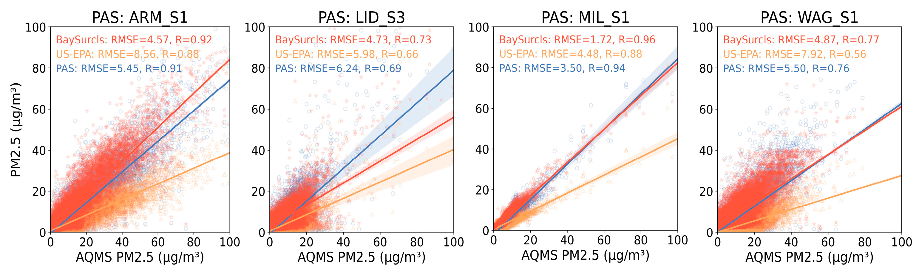
Figure 10.
Example of time series plots for two PASs for a two week period, comparing the reference PM2.5 data with relevant raw PAS2.5 data and PAS2.5 data corrected with the US-EPA method or the BaySurcls model.
Figure 10.
Example of time series plots for two PASs for a two week period, comparing the reference PM2.5 data with relevant raw PAS2.5 data and PAS2.5 data corrected with the US-EPA method or the BaySurcls model.
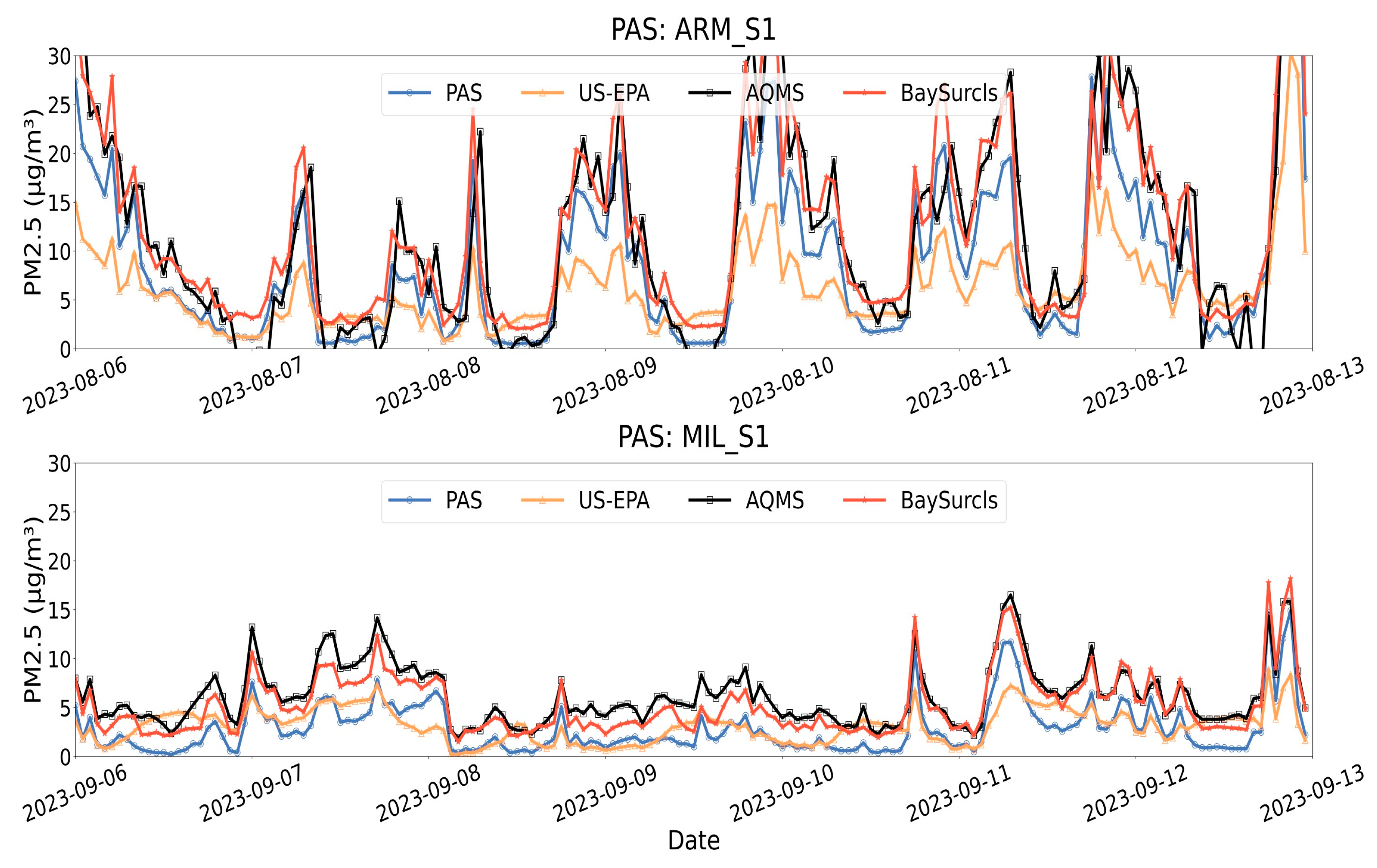
Time series plots for raw PAS data, corrected PAS data, and reference PM2.5 data further confirm BaySurcls's superior correction capabilities. Figure 9 gives examples of scatter plots for two sensors. Throughout the two-week periods analysed, BaySurcls closely aligned with the reference PM2.5 data, accurately capturing both peaks and troughs. In contrast, the uncorrected PAS PM2.5 data often showed a steady underestimation, while the US-EPA method-corrected data frequently failed to capture the full amplitude of pollution spikes. This further highlights BaySurcls’s ability to deliver improved PAS PM2.5 data for the non-collocation monitoring scenario, i.e., PAS monitoring at locations without direct reference measurements.
We also examined the violin plots for the ratios of the reference PM2.5 to the raw PAS2.5 data or PAS2.5 data corrected with the BaySurcls model or the US-EPA method, under the non-collocation monitoring scenario. Figure 11 shows example violin plots for for two sensors. The raw PAS data exhibits some significant spread and variability, particularly across all months. In contrast, the BaySurcls model maintained narrower distributions of ratios, showing less variability and greater precision in corrected PAS data (i.e., higher accuracy in aligning with the reference data). However, the PAS data corrected with the US-EPA method exhibited much larger spread and variability, comparable to those for the raw PAS data, indicating limited applicability in the context of NSW.
These findings underscore the robustness and reliability of the BaySurcls model in enhancing the quality of PM2.5 data from PASs, even in the absence of collocated reference stations. By accounting for local variability and learning from multiple sensors, BaySurcls provides a more adaptable solution for accurate air quality monitoring in different environments, making it an essential tool for ensuring data quality in regions lacking regulatory-grade monitoring.
4. Summary and Conclusion
PurpleAir sensors have been applied in PM2.5 monitoring in many regions in the world, primarily due to its affordability, portability, low power demand and easy maintenance. However, the measurement accuracy of such sensors can be influenced by environmental factors such as temperature, humidity and emission types. Therefore, PAS measurements must be corrected to provide PM2.5 data compatible to those from regulatory monitors, prior to its use for air quality reporting or research. One of the mostly used correction methods is the on derived by the US-EPA that consider the effects of relative humidity on PAS measurement accuracy [10].This study has examined the applicability the US-EPA method in the NSW context, and explored the potential for applying ML/DL algorithms to formulate new methods for PAS data correction in the region. The investigation was undertaken for two situations: (1) data correction for PAS monitoring where there exists collocated (standard) compliance monitoring (i.e., the collocation monitoring scenario); and (2) data correction for PAS monitoring where there is no collocated standard monitoring (the non-collocation scenario). The main findings are summarised below:
- The US-EPA method showed limited skills for correcting PAS data under both collocation and non-collocation monitoring scenarios, thus deemed inappropriate for common application in NSW.
- In contrast, the ML/DL methods tested in this study generally showed much superior performance over the US-EPA method at the tested locations.
- Among the tested algorithms, the hybrid model BaySurcls, featuring the application of deep learning (DL) algorithms in conjunction with a Bayesian-optimized surrogate model, showed good promise as a tool for improving PAS PM2.5 measurement accuracy.
- The BaySurcls and other ML/DL-based methods demonstrated high-level skills for correcting PAS data under the collocation scenario, and generally moderate-to high-level skills under the non-collocation scenario.
- The Performance of both ML/DL based methods and the US-EPA method could vary significantly across different air quality regions, indicating a need for further research in developing rigorous methods for correcting PAS data in NSW.
In conclusion, this study has demonstrated a good promise in developing more efficient method for correcting the PAS monitoring data by leveraging advanced architectures of ML/DL models. One area for improvement is leveraging transfer learning techniques to enable models trained on one region’s data to be adapted efficiently for use in other regions with minimal retraining. Integrating deep learning with dynamic quantile regression in BaySurcls makes it possible to refine PurpleAir sensor (PAS) that can be helpful not only to adjusts the changing conditions but also helps to estimate the uncertainties, leading to a more reliable and accurate correction.
Data correction skills can also be tested on models which include data from a wider range of stations, particularly those in diverse geographic regions with varying climatic and environmental conditions. This will enhance the model’s ability to generalise across different landscapes and environmental settings. Another direction is to explore the adaptability of the (less complex) US-EPA approach in the NSW context, if additional collocated data are made available from more locations and across different regions. This study will form the foundation of further work on data fusion, impact assessment and air quality nowcasting and forecasting in NSW. The results and approach can also be useful for other jurisdictions in Australia, or similar regions elsewhere
Author Contributions
Conceptualization, Masrur Ahmed,Ningbo Jiang, and Jing Kong; methodology, Masrur Ahmed,Ningbo Jiang, and Jing Kong; software, Masrur Ahmed, Jing Kong; formal analysis, Masrur Ahmed and Jing Kong; model development, Masrur Ahmed; investigation, Masrur Ahmed; data curation, Jing Kong and Praveen Puppala; visualization, Masrur Ahmed and Jing Kong; writing—original draft preparation, Masrur Ahmed and Jing Kong; writing—review and editing, Masrur Ahmed,Ningbo Jiang, Jing Kong, Hiep Nguyen Duc, Praveen Puppala, Merched Azzi, Matthew Riley, and Xavier Barthelemy.
Funding
The New South Wales Air Quality Monitoring Network is funded and maintained by Department of Climate Change, Energy, the Environment and Water (DCCEEW), New South Wales Government.
Data Availability Statement
The air quality data from the New South Wales Air Quality Monitoring Network are freely downloadable via DCCEEW’s air quality data API (Application Programming Interface) at https://www.airquality.nsw.gov.au/air-quality-data-services/air-quality-api.
Acknowledgments
We acknowledge the permission for access PurpleAir data via https://community.purpleair.com/c/data/7 (accessed July 2024).
Conflicts of Interest
The authors declare that they have no conflicts of interest.
References
- Anenberg, S.C.; Belova, A.; Brandt, J.; Fann, N.; Greco, S.; Guttikunda, S.; Heroux, M.E.; Hurley, F.; Krzyzanowski, M.; Medina, S. Survey of ambient air pollution health risk assessment tools. Risk analysis 2016, 36, 1718–1736. [Google Scholar] [CrossRef]
- De Marco, A.; Proietti, C.; Anav, A.; Ciancarella, L.; D'Elia, I.; Fares, S.; Fornasier, M.F.; Fusaro, L.; Gualtieri, M.; Manes, F. Impacts of air pollution on human and ecosystem health, and implications for the National Emission Ceilings Directive: Insights from Italy. Environment International 2019, 125, 320–333. [Google Scholar] [CrossRef] [PubMed]
- Robinson, D.L. Accurate, low cost PM2. 5 measurements demonstrate the large spatial variation in wood smoke pollution in regional Australia and improve modeling and estimates of health costs. Atmosphere 2020, 11, 856. [Google Scholar] [CrossRef]
- Aini, Q.; Febriani, W.; Lukita, C.; Kosasi, S.; Rahardja, U. New normal regulation with face recognition technology using attendx for student attendance algorithm. In Proceedings of the 2022 International Conference on Science and Technology (ICOSTECH), 2022; pp. 1-7.
- Dominici, F.; Peng, R.D.; Zeger, S.L.; White, R.H.; Samet, J.M. Particulate air pollution and mortality in the United States: did the risks change from 1987 to 2000? American Journal of Epidemiology 2007, 166, 880–888. [Google Scholar] [CrossRef]
- Franklin, M.; Zeka, A.; Schwartz, J. Association between PM2. 5 and all-cause and specific-cause mortality in 27 US communities. Journal of exposure science & environmental epidemiology 2007, 17, 279–287. [Google Scholar]
- Di, Q.; Dai, L.; Wang, Y.; Zanobetti, A.; Choirat, C.; Schwartz, J.D.; Dominici, F. Association of short-term exposure to air pollution with mortality in older adults. Jama 2017, 318, 2446–2456. [Google Scholar] [CrossRef] [PubMed]
- Bell, M.L.; Ebisu, K.; Belanger, K. Ambient air pollution and low birth weight in Connecticut and Massachusetts. Environmental health perspectives 2007, 115, 1118–1124. [Google Scholar] [CrossRef]
- Grande, G.; Ljungman, P.L.; Eneroth, K.; Bellander, T.; Rizzuto, D. Association between cardiovascular disease and long-term exposure to air pollution with the risk of dementia. JAMA neurology 2020, 77, 801–809. [Google Scholar] [CrossRef]
- Barkjohn, K.K.; Gantt, B.; Clements, A.L. Development and application of a United States-wide correction for PM 2.5 data collected with the PurpleAir sensor. Atmospheric Measurement Techniques 2021, 14, 4617–4637. [Google Scholar] [CrossRef]
- Ahmed, A.A.M.; Jui, S.J.J.; Sharma, E.; Ahmed, M.H.; Raj, N.; Bose, A. An advanced deep learning predictive model for air quality index forecasting with remote satellite-derived hydro-climatological variables. Sci Total Environ 2024, 906, 167234. [Google Scholar] [CrossRef]
- Marshall, J.D.; Nethery, E.; Brauer, M. Within-urban variability in ambient air pollution: comparison of estimation methods. Atmospheric Environment 2008, 42, 1359–1369. [Google Scholar] [CrossRef]
- Tan, Y.; Lipsky, E.M.; Saleh, R.; Robinson, A.L.; Presto, A.A. Characterizing the spatial variation of air pollutants and the contributions of high emitting vehicles in Pittsburgh, PA. Environmental science & technology 2014, 48, 14186–14194. [Google Scholar]
- Zimmerman, N.; Presto, A.A.; Kumar, S.P.; Gu, J.; Hauryliuk, A.; Robinson, E.S.; Robinson, A.L.; Subramanian, R. Closing the gap on lower cost air quality monitoring: Machine learning calibration models to improve low-cost sensor performance. Atmos. Meas. Tech. Discuss 2017, 2017, 1–36. [Google Scholar]
- Rahardja, U.; Aini, Q.; Manongga, D.; Sembiring, I.; Sanjaya, Y.P.A. Enhancing machine learning with low-cost p m2. 5 air quality sensor calibration using image processing. APTISI Transactions on Management 2023, 7, 201–209. [Google Scholar]
- Lewis, A.; Edwards, P. Validate personal air-pollution sensors. Nature 2016, 535, 29–31. [Google Scholar] [CrossRef]
- McKercher, G.R.; Salmond, J.A.; Vanos, J.K. Characteristics and applications of small, portable gaseous air pollution monitors. Environmental Pollution 2017, 223, 102–110. [Google Scholar] [CrossRef] [PubMed]
- Moltchanov, S.; Levy, I.; Etzion, Y.; Lerner, U.; Broday, D.M.; Fishbain, B. On the feasibility of measuring urban air pollution by wireless distributed sensor networks. Science of The Total Environment 2015, 502, 537–547. [Google Scholar] [CrossRef]
- Snyder, E.G.; Watkins, T.H.; Solomon, P.A.; Thoma, E.D.; Williams, R.W.; Hagler, G.S.; Shelow, D.; Hindin, D.A.; Kilaru, V.J.; Preuss, P.W. The changing paradigm of air pollution monitoring. Environmental science & technology 2013, 47, 11369–11377. [Google Scholar]
- Jaffe, D.A.; Thompson, K.; Finley, B.; Nelson, M.; Ouimette, J.; Andrews, E. An evaluation of the US EPA's correction equation for PurpleAir sensor data in smoke, dust, and wintertime urban pollution events. Atmospheric Measurement Techniques 2023, 16, 1311–1322. [Google Scholar] [CrossRef]
- Jayaratne, R.; Liu, X.; Thai, P.; Dunbabin, M.; Morawska, L. The influence of humidity on the performance of a low-cost air particle mass sensor and the effect of atmospheric fog. Atmospheric Measurement Techniques 2018, 11, 4883–4890. [Google Scholar] [CrossRef]
- Zheng, T.; Bergin, M.H.; Johnson, K.K.; Tripathi, S.N.; Shirodkar, S.; Landis, M.S.; Sutaria, R.; Carlson, D.E. Field evaluation of low-cost particulate matter sensors in high-and low-concentration environments. Atmospheric Measurement Techniques 2018, 11, 4823–4846. [Google Scholar] [CrossRef]
- Masson, N.; Piedrahita, R.; Hannigan, M. Quantification method for electrolytic sensors in long-term monitoring of ambient air quality. Sensors 2015, 15, 27283–27302. [Google Scholar] [CrossRef] [PubMed]
- Pang, X.; Shaw, M.D.; Lewis, A.C.; Carpenter, L.J.; Batchellier, T. Electrochemical ozone sensors: A miniaturised alternative for ozone measurements in laboratory experiments and air-quality monitoring. Sensors and Actuators B: Chemical 2017, 240, 829–837. [Google Scholar] [CrossRef]
- Williams, D.E.; Henshaw, G.S.; Bart, M.; Laing, G.; Wagner, J.; Naisbitt, S.; Salmond, J.A. Validation of low-cost ozone measurement instruments suitable for use in an air-quality monitoring network. Measurement Science and Technology 2013, 24, 065803. [Google Scholar] [CrossRef]
- Tryner, J.; Mehaffy, J.; Miller-Lionberg, D.; Volckens, J. Effects of aerosol type and simulated aging on performance of low-cost PM sensors. Journal of Aerosol Science 2020, 150, 105654. [Google Scholar] [CrossRef]
- Ardon-Dryer, K.; Dryer, Y.; Williams, J.N.; Moghimi, N. Measurements of PM 2.5 with PurpleAir under atmospheric conditions. Atmospheric Measurement Techniques 2020, 13, 5441–5458. [Google Scholar] [CrossRef]
- Kelly, K.; Whitaker, J.; Petty, A.; Widmer, C.; Dybwad, A.; Sleeth, D.; Martin, R.; Butterfield, A. Ambient and laboratory evaluation of a low-cost particulate matter sensor. Environmental pollution 2017, 221, 491–500. [Google Scholar] [CrossRef]
- Malings, C.; Tanzer, R.; Hauryliuk, A.; Saha, P.K.; Robinson, A.L.; Presto, A.A.; Subramanian, R. Fine particle mass monitoring with low-cost sensors: Corrections and long-term performance evaluation. Aerosol Science and Technology 2020, 54, 160–174. [Google Scholar] [CrossRef]
- Magi, B.I.; Cupini, C.; Francis, J.; Green, M.; Hauser, C. Evaluation of PM2. 5 measured in an urban setting using a low-cost optical particle counter and a Federal Equivalent Method Beta Attenuation Monitor. Aerosol Science and Technology 2020, 54, 147–159. [Google Scholar] [CrossRef]
- Bi, J.; Wildani, A.; Chang, H.H.; Liu, Y. Incorporating low-cost sensor measurements into high-resolution PM2. 5 modeling at a large spatial scale. Environmental Science & Technology 2020, 54, 2152–2162. [Google Scholar]
- Feenstra, B.; Papapostolou, V.; Hasheminassab, S.; Zhang, H.; Der Boghossian, B.; Cocker, D.; Polidori, A. Performance evaluation of twelve low-cost PM2. 5 sensors at an ambient air monitoring site. Atmospheric Environment 2019, 216, 116946. [Google Scholar] [CrossRef]
- Mehadi, A.; Moosmüller, H.; Campbell, D.E.; Ham, W.; Schweizer, D.; Tarnay, L.; Hunter, J. Laboratory and field evaluation of real-time and near real-time PM2. 5 smoke monitors. Journal of the Air & Waste Management Association 2020, 70, 158–179. [Google Scholar]
- Schulte, N.; Li, X.; Ghosh, J.K.; Fine, P.M.; Epstein, S.A. Responsive high-resolution air quality index mapping using model, regulatory monitor, and sensor data in real-time. Environmental Research Letters 2020, 15, 1040a1047. [Google Scholar] [CrossRef]
- Lu, Y.; Giuliano, G.; Habre, R. Estimating hourly PM2. 5 concentrations at the neighborhood scale using a low-cost air sensor network: A Los Angeles case study. Environmental Research 2021, 195, 110653. [Google Scholar] [CrossRef] [PubMed]
- Kim, S.; Park, S.; Lee, J. Evaluation of performance of inexpensive laser based PM2. 5 sensor monitors for typical indoor and outdoor hotspots of South Korea. Applied Sciences 2019, 9, 1947. [Google Scholar] [CrossRef]
- Stavroulas, I.; Grivas, G.; Michalopoulos, P.; Liakakou, E.; Bougiatioti, A.; Kalkavouras, P.; Fameli, K.M.; Hatzianastassiou, N.; Mihalopoulos, N.; Gerasopoulos, E. Field evaluation of low-cost PM sensors (Purple Air PA-II) under variable urban air quality conditions, in Greece. Atmosphere 2020, 11, 926. [Google Scholar] [CrossRef]
- Dhammapala, R.; Basnayake, A.; Premasiri, S.; Chathuranga, L.; Mera, K. PM2. 5 in Sri Lanka: Trend analysis, low-cost sensor correlations and spatial distribution. Aerosol and Air Quality Research 2022, 22, 210266. [Google Scholar] [CrossRef]
- McFarlane, C.; Isevulambire, P.K.; Lumbuenamo, R.S.; Ndinga, A.M.E.; Dhammapala, R.; Jin, X.; McNeill, V.F.; Malings, C.; Subramanian, R.; Westervelt, D.M. First measurements of ambient PM2. 5 in Kinshasa, Democratic Republic of Congo and Brazzaville, Republic of Congo using field-calibrated low-cost sensors. Aerosol and Air Quality Research 2021, 21, 200619. [Google Scholar] [CrossRef]
- Chojer, H.; Branco, P.; Martins, F.; Alvim-Ferraz, M.; Sousa, S. Can data reliability of low-cost sensor devices for indoor air particulate matter monitoring be improved?–An approach using machine learning. Atmospheric Environment 2022, 286, 119251. [Google Scholar] [CrossRef]
- Yu, M.; Zhang, S.; Zhang, K.; Yin, J.; Varela, M.; Miao, J. Developing high-resolution PM2. 5 exposure models by integrating low-cost sensors, automated machine learning, and big human mobility data. Frontiers in Environmental Science 2023, 11, 1223160. [Google Scholar] [CrossRef]
- Kar, A.; Ahmed, M.; May, A.A.; Le, H.T. High spatio-temporal resolution predictions of PM2. 5 using low-cost sensor data. Atmospheric Environment 2024, 326, 120486. [Google Scholar] [CrossRef]
- Paton-Walsh, C.; Rayner, P.; Simmons, J.; Fiddes, S.L.; Schofield, R.; Bridgman, H.; Beaupark, S.; Broome, R.; Chambers, S.D.; Chang, L.T.-C. A clean air plan for Sydney: An overview of the special issue on air quality in New South Wales. Atmosphere 2019, 10, 774. [Google Scholar] [CrossRef]
- Barnett, A.G.; Williams, G.M.; Schwartz, J.; Best, T.L.; Neller, A.H.; Petroeschevsky, A.L.; Simpson, R.W. The effects of air pollution on hospitalizations for cardiovascular disease in elderly people in Australian and New Zealand cities. Environmental health perspectives 2006, 114, 1018–1023. [Google Scholar] [CrossRef]
- Cohen, D.D.; Stelcer, E.; Garton, D.; Crawford, J. Fine particle characterisation, source apportionment and long-range dust transport into the Sydney Basin: a long term study between 1998 and 2009. Atmospheric Pollution Research 2011, 2, 182–189. [Google Scholar] [CrossRef]
- Cope, M.; Keywood, M.; Emmerson, K.; Galbally, I.; Boast, K.; Chambers, S.; Cheng, M.; Crumeyrolle, S.; Dunne, E.; Fedele, R. Sydney particle study-stage-II; CSIRO Marine and Atmospheric Research: 2014.
- Barkjohn, K.K.; Gantt, B.; Clements, A.L. Development and Application of a United States wide correction for PM(2.5) data collected with the PurpleAir sensor. Atmos Meas Tech 2021, 4. [Google Scholar] [CrossRef]
- Ardon-Dryer, K.; Dryer, Y.; Williams, J.N.; Moghimi, N. Measurements of PM2.5 with PurpleAir under atmospheric conditions. Atmospheric Measurement Techniques 2020, 13, 5441–5458. [Google Scholar] [CrossRef]
- Magi, B.I.; Cupini, C.; Francis, J.; Green, M.; Hauser, C. Evaluation of PM2.5 measured in an urban setting using a low-cost optical particle counter and a Federal Equivalent Method Beta Attenuation Monitor. Aerosol Science and Technology 2019, 54, 147–159. [Google Scholar] [CrossRef]
- Si, M.; Xiong, Y.; Du, S.; Du, K. Evaluation and calibration of a low-cost particle sensor in ambient conditions using machine-learning methods. Atmospheric Measurement Techniques 2020, 13, 1693–1707. [Google Scholar] [CrossRef]
- Masrur Ahmed, A.A.; Akther, S.; Nguyen-Huy, T.; Raj, N.; Janifer Jabin Jui, S.; Farzana, S.Z. Real-time prediction of the week-ahead flood index using hybrid deep learning algorithms with synoptic climate mode indices. Journal of Hydro-environment Research 2024, 57, 12–26. [Google Scholar] [CrossRef]
- Akbari Asanjan, A.; Yang, T.; Hsu, K.; Sorooshian, S.; Lin, J.; Peng, Q. Short-Term Precipitation Forecast Based on the PERSIANN System and LSTM Recurrent Neural Networks. Journal of Geophysical Research: Atmospheres 2018, 123. [Google Scholar] [CrossRef]
- Aungiers, J. Time Series Prediction Using LSTM Deep Neural Networks. 2018.
- Huang, C.J.; Kuo, P.H. A Deep CNN-LSTM Model for Particulate Matter (PM2.5) Forecasting in Smart Cities. Sensors (Basel) 2018, 18. [Google Scholar] [CrossRef] [PubMed]
- Wang, J.; Li, X.; Jin, L.; Li, J.; Sun, Q.; Wang, H. An air quality index prediction model based on CNN-ILSTM. Sci Rep 2022, 12, 8373. [Google Scholar] [CrossRef] [PubMed]
- Jui, S.J.J.; Ahmed, A.A.M.; Bose, A.; Raj, N.; Sharma, E.; Soar, J.; Chowdhury, M.W.I. Spatiotemporal Hybrid Random Forest Model for Tea Yield Prediction Using Satellite-Derived Variables. Remote Sensing 2022, 14. [Google Scholar] [CrossRef]
- Hochreiter, S. Long Short-term Memory. Neural Computation MIT-Press 1997.
- Beretta, L.; Santaniello, A. Nearest neighbor imputation algorithms: a critical evaluation. BMC Med Inform Decis Mak 2016, 16 Suppl 3, 74. [Google Scholar] [CrossRef]
- Cabello-Solorzano, K.; Ortigosa de Araujo, I.; Peña, M.; Correia, L.; J. Tallón-Ballesteros, A. The impact of data normalization on the accuracy of machine learning algorithms: a comparative analysis. In Proceedings of the International Conference on Soft Computing Models in Industrial and Environmental Applications, 2023; pp. 344-353.
- Chen, T.; Guestrin, C. Xgboost: A scalable tree boosting system. In Proceedings of the Proceedings of the 22nd acm sigkdd international conference on knowledge discovery and data mining, 2016; pp. 785-794.
- Snoek, J.; Larochelle, H.; Adams, R.P. Practical bayesian optimization of machine learning algorithms. Advances in neural information processing systems 2012, 25. [Google Scholar]
- Snoek, J.; Rippel, O.; Swersky, K.; Kiros, R.; Satish, N.; Sundaram, N.; Patwary, M.; Prabhat, M.; Adams, R. Scalable bayesian optimization using deep neural networks. In Proceedings of the International conference on machine learning, 2015; pp. 2171-2180.
- Frazier, P.I. Bayesian optimization. In Recent advances in optimization and modeling of contemporary problems; Informs: 2018; pp. 255-278.
Figure 1.
Location of air quality monitoring stations (AQMSs) (blue dots on map) and collocated PurpleAir sensors (PASs) (dot linked and listed on the right). PASs are highlighted blue if used for the purpose of building transfer learning models under the non-collocation monitoring scenario.
Figure 1.
Location of air quality monitoring stations (AQMSs) (blue dots on map) and collocated PurpleAir sensors (PASs) (dot linked and listed on the right). PASs are highlighted blue if used for the purpose of building transfer learning models under the non-collocation monitoring scenario.
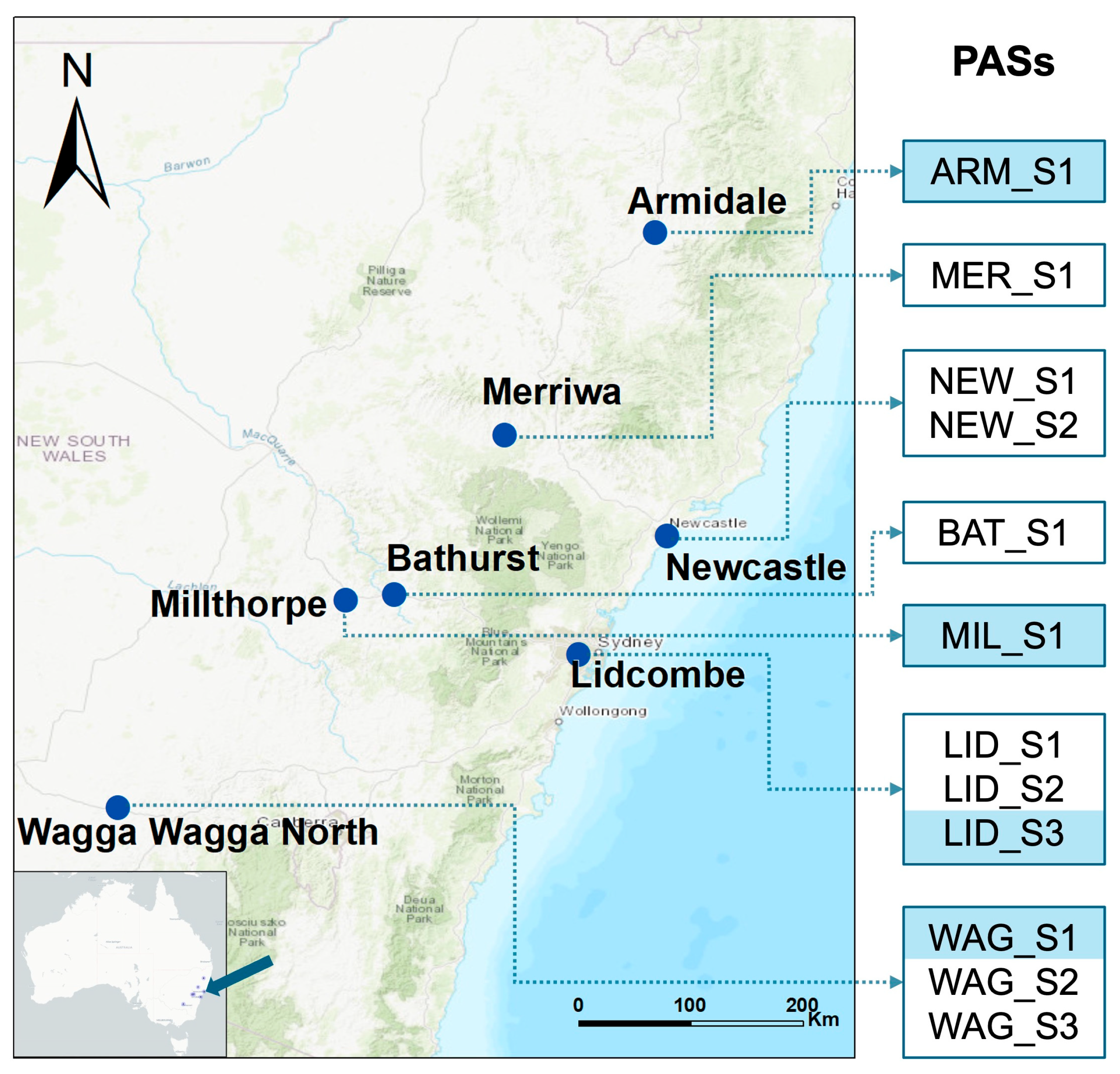
Figure 2.
Boxplots of PM 2.5 data ratio between AQMS and collocated PAS readings (horizontal line in box indicates median value position).
Figure 2.
Boxplots of PM 2.5 data ratio between AQMS and collocated PAS readings (horizontal line in box indicates median value position).
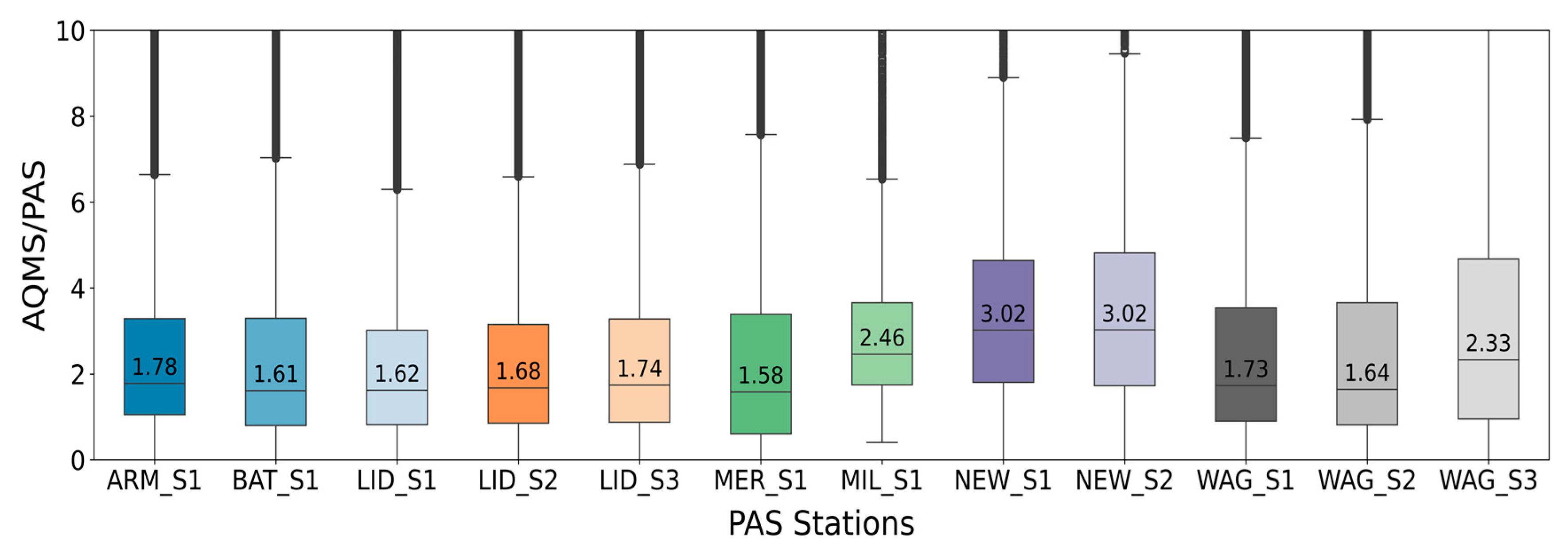
Figure 3.
Workflow of the BaySurcls framework for correcting PurpleAir sensor PM2.5 Data.
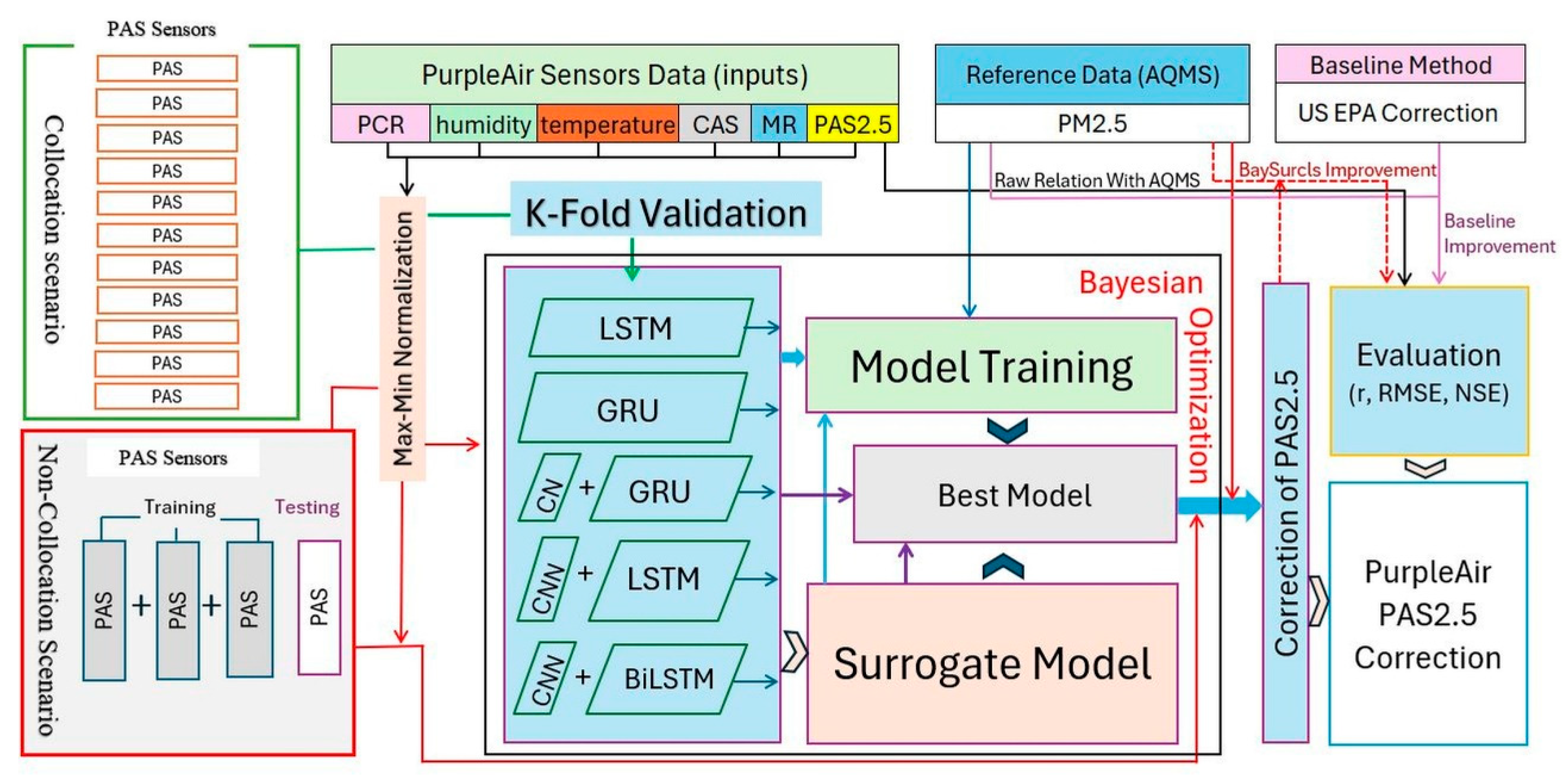
Figure 4.
Correction efficiencies expressed in NSE values for tested ML/DL based methods compared to the US-EPA method for each collocated PAS.
Figure 4.
Correction efficiencies expressed in NSE values for tested ML/DL based methods compared to the US-EPA method for each collocated PAS.
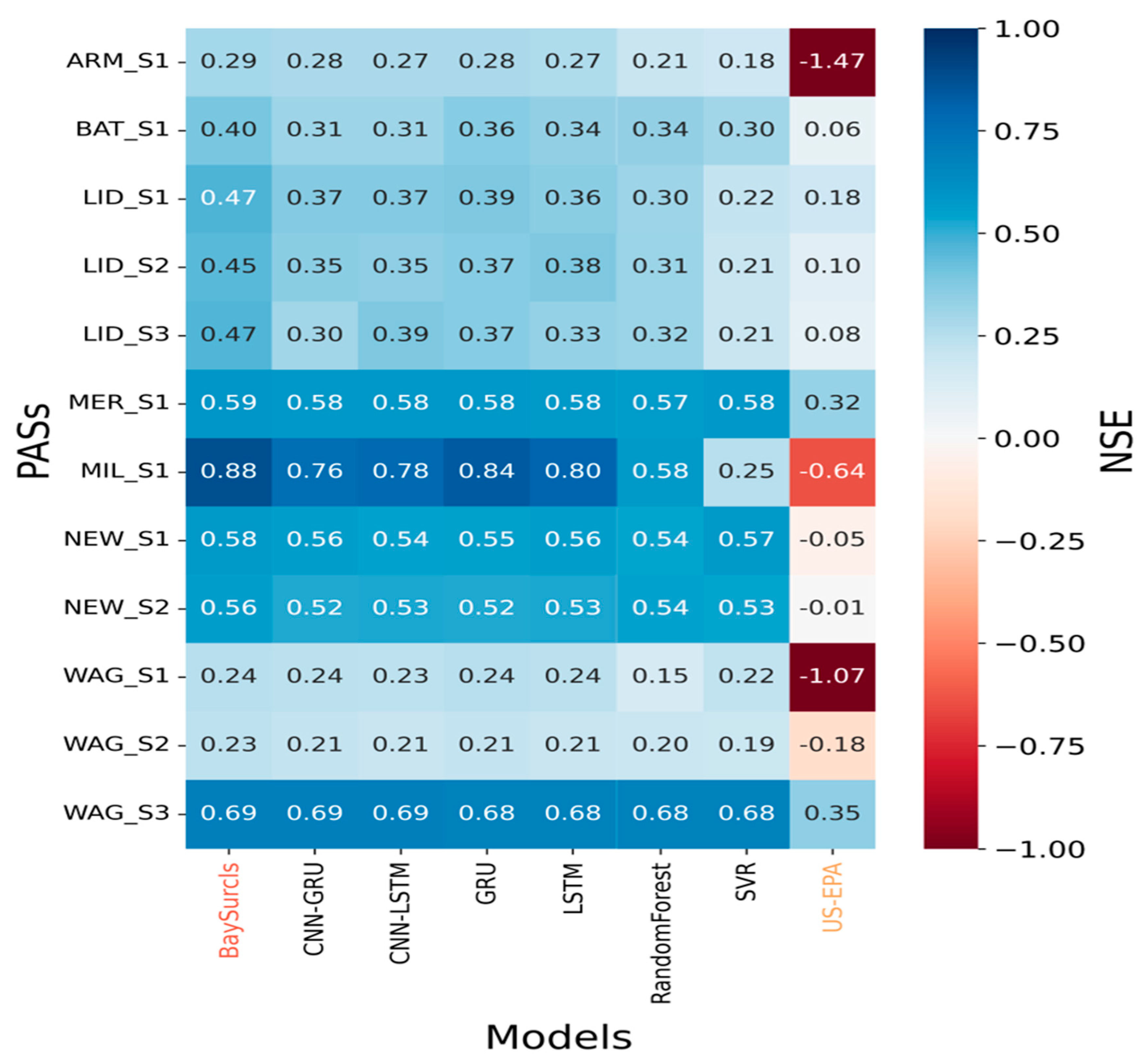
Figure 5.
Scatter plots demonstrating the correlation (R) between the reference PM2.5 data and: the raw PAS data (blue), the US-EPA-corrected PM2.5 (orange), and the BaySurcls-corrected PM2.5 (red), as well as the improvement in RMSE by applying different correction methods, under the collocation monitoring scenario.
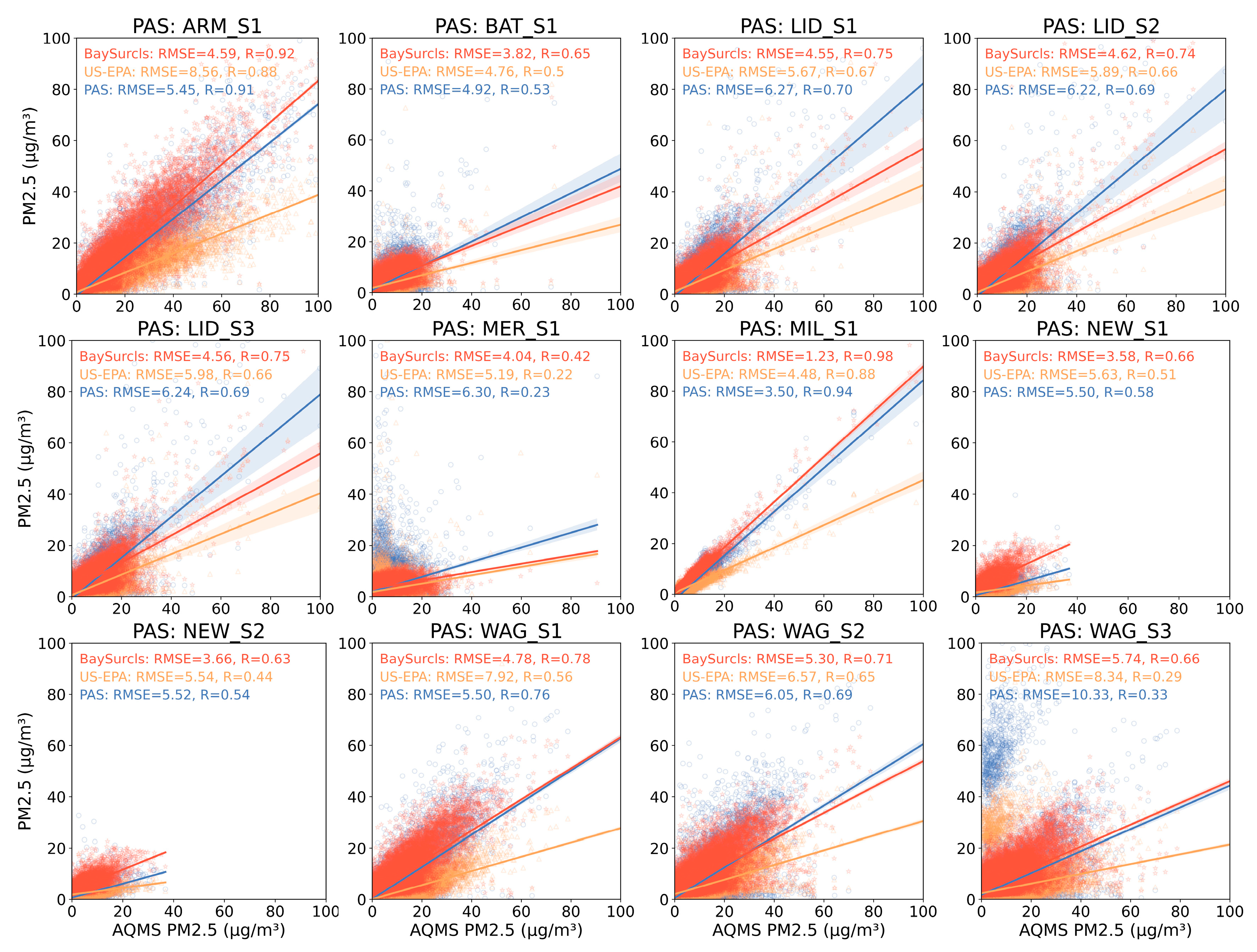
Figure 6.
Example time series plots for two typical cases of high and low ambient PM2.5 pollution, comparing the raw PAS, US-EPA-corrected and BaySurcls-corrected data with the reference PM2.5 data.
Figure 6.
Example time series plots for two typical cases of high and low ambient PM2.5 pollution, comparing the raw PAS, US-EPA-corrected and BaySurcls-corrected data with the reference PM2.5 data.
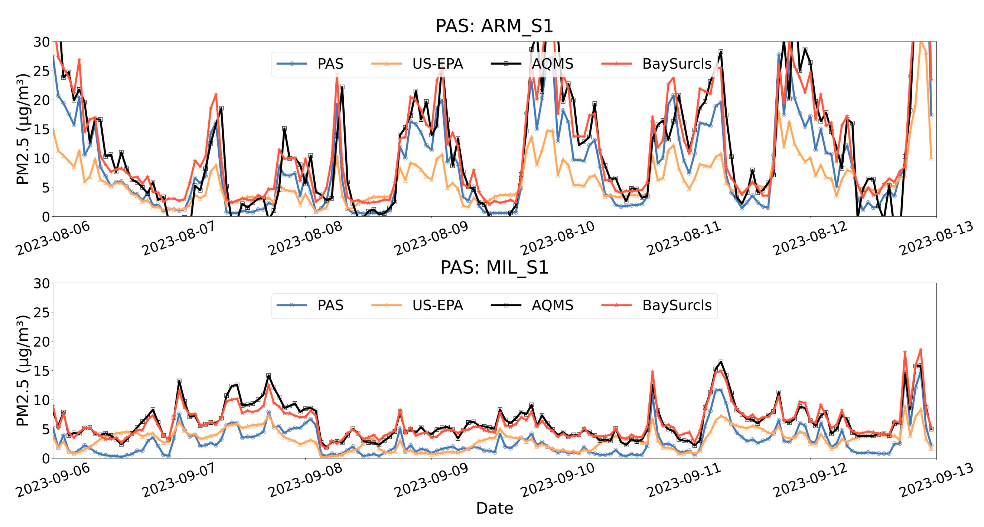
Figure 7.
Example violin plots - illustrating the monthly distribution of the ratios between reference (AQMS) PM2.5 data and: (1) raw PAS2.5 data (blue), (2) corrected PAS2.5 data with the US-EPA method, and (3) corrected PAS2.5 with BaySurcls (brown) for two sensors in the collocation monitoring scenario. January to December is indicated by 1 to 12.
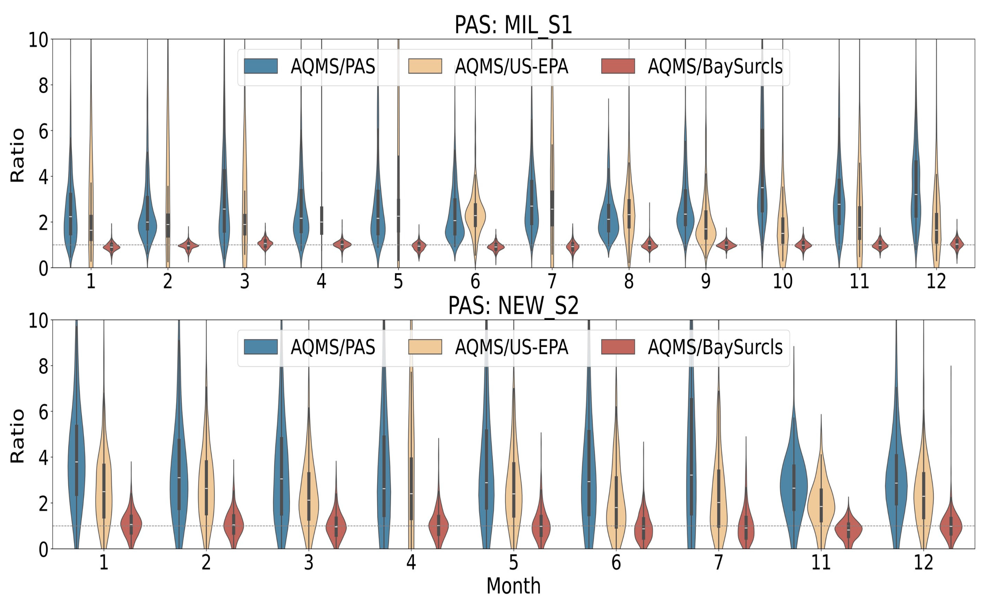
Figure 8.
Correction efficiencies expressed in NSE for ML/DL based models and the US-EPA method for correcting the PAS PM2.5 for PAS monitoring scenario where no collocated reference monitoring exists.
Figure 8.
Correction efficiencies expressed in NSE for ML/DL based models and the US-EPA method for correcting the PAS PM2.5 for PAS monitoring scenario where no collocated reference monitoring exists.
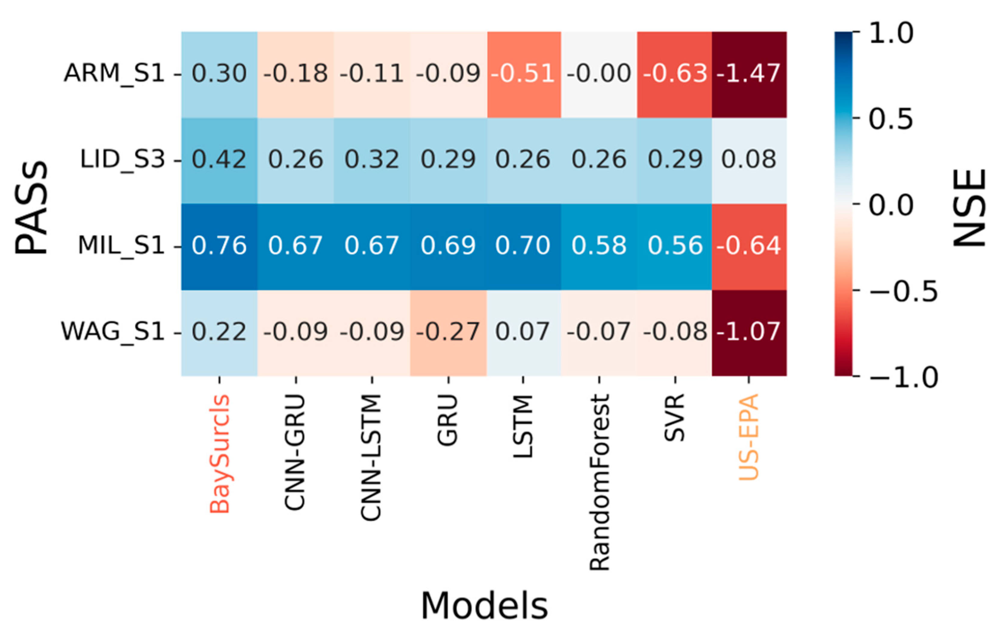
Figure 11.
Violin plot presents the monthly distribution of the ratio between PM2.5/PAS PM2.5 and PM2.5/BaySurcls-calibrated PM2.5 for selected collocated sensors.
Figure 11.
Violin plot presents the monthly distribution of the ratio between PM2.5/PAS PM2.5 and PM2.5/BaySurcls-calibrated PM2.5 for selected collocated sensors.
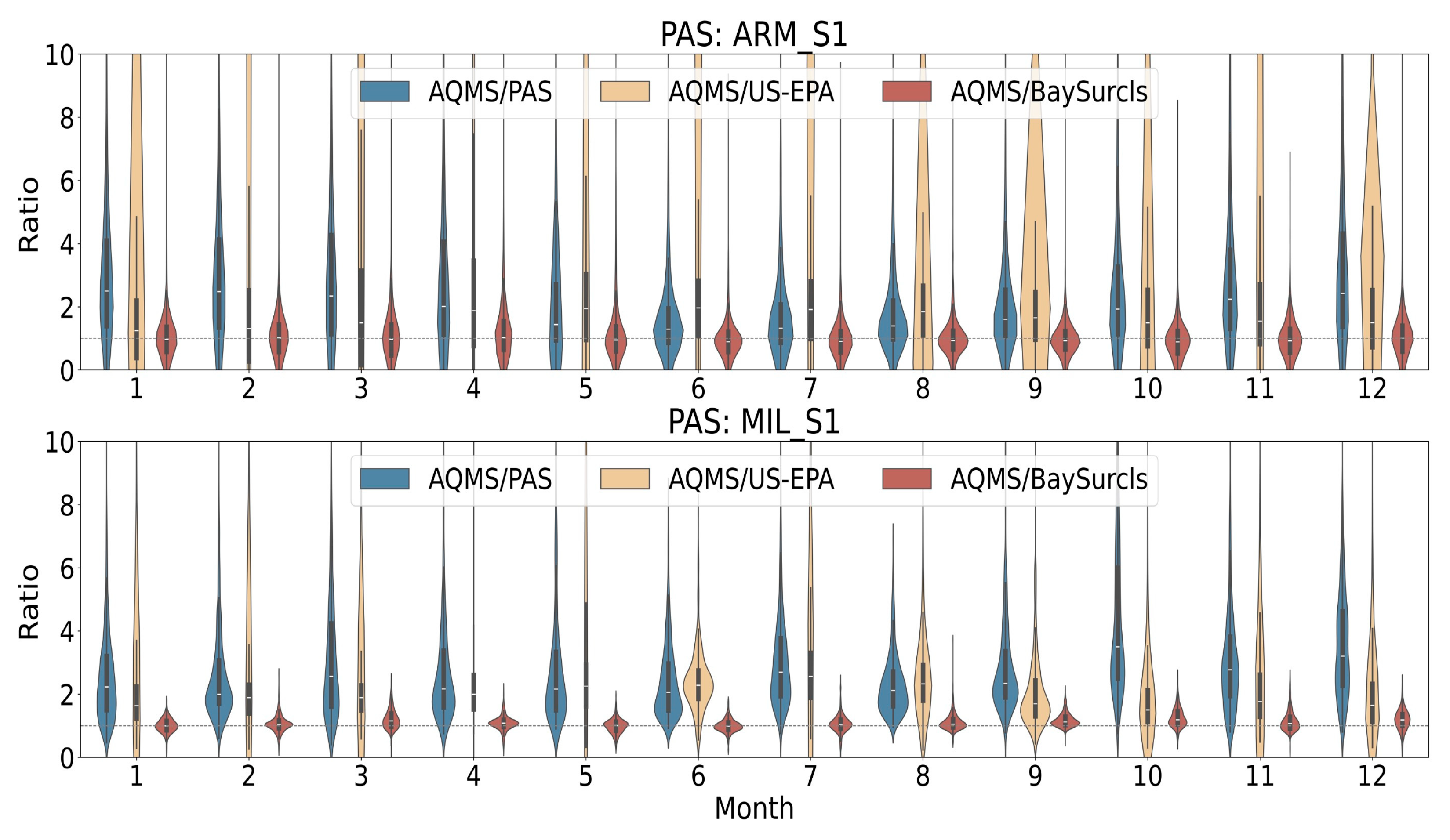

Table 1.
Details of air quality monitoring stations and corresponding co-located PurpleAir sensors and data period.
Table 1.
Details of air quality monitoring stations and corresponding co-located PurpleAir sensors and data period.
| Region Name | AQMS Name | Latitude | Longitude | PAS ID (online) |
PAS Name | Data Period |
|---|---|---|---|---|---|---|
| Riverina-Murray | Wagga Wagga North | 29959 | WAG_S1 | 01/03/2020 – 16/07/2024 | ||
| -35.10411 | 147.36037 | 29945 | WAG2 | 01/03/2020 – 16/07/2024 | ||
| 30007 | WAG3 | 01/03/2020 – 16/07/2024 | ||||
| Northern Tablelands | Armidale | -30.50851 | 151.66173 | 29949 | ARM1 | 01/03/2020 – 16/07/2024 |
| Sydney | Lidcombe | 91721 | LID1 | 08/02/2021 - 16/07/2024 | ||
| -33.88143 | 151.04676 | 92367 | LID2 | 15/02/2021 - 16/07/2024 | ||
| 91355 | LID3 | 15/02/2021 - 16/07/2024 | ||||
| Central Tablelands | Bathurst | -33.40178 | 149.57456 | 98435 | BAT1 | 28/05/2021 – 16/07/2024 |
| Millthorpe | -33.444339 | 149.185325 | 182853 | MIL1 | 26/07/2023 – 30/07/2024 | |
| Lower Hunter | Newcastle | -32.9312 | 151.75965 | 191067 | NEW1 | 15/11/2023 – 16/07/2024 |
| 191081 | NEW2 | 15/11/2023 – 16/07/2024 | ||||
| Upper Hunter | Merriwa | -32.12665 | 150.45824 | 92479 | MER1 | 09/02/2021 – 30/07/2024 |
Table 2.
Aerosol and Particle Ratios Used for PM2.5 Calibration.
| Ratio Name | Calculation | Significance |
|---|---|---|
| Coarse Aerosol Fraction (CAF) | CAF = (PM10 −PM2.5)/PM10 | High CAF (> 0.5): coarse particles, likely dust. Low CAF (< 0.5): fine particles, typical of smoke or urban pollution. |
| Mass Ratio (MR) | MR = PM1/PM10 | High MR (> 0.5): More ultrafine particles, likely from smoke or combustion. Low MR (< 0.5): More large particles, typical of dust. |
| Particle Count Ratio (PCR) | PCR = 0.3 µm /5µm | High PCR (> 500): Dominance of fine particles, indicating smoke. Low PCR (< 500): More coarse particles, suggesting dust. |
Disclaimer/Publisher’s Note: The statements, opinions and data contained in all publications are solely those of the individual author(s) and contributor(s) and not of MDPI and/or the editor(s). MDPI and/or the editor(s) disclaim responsibility for any injury to people or property resulting from any ideas, methods, instructions or products referred to in the content. |
© 2024 by the authors. Licensee MDPI, Basel, Switzerland. This article is an open access article distributed under the terms and conditions of the Creative Commons Attribution (CC BY) license (http://creativecommons.org/licenses/by/4.0/).
Copyright: This open access article is published under a Creative Commons CC BY 4.0 license, which permit the free download, distribution, and reuse, provided that the author and preprint are cited in any reuse.


