Submitted:
25 October 2024
Posted:
28 October 2024
You are already at the latest version
Abstract
Treatment efficacy for age-related macular degeneration relies on early diagnosis and precise determination of the disease stage. It involves analyzing biomarkers in retinal images, which can be challenging when handling a large flow of patients and compromise the quality of healthcare services. Clinical decision support systems offer a solution to this issue by employing intelligent algorithms to recognize biomarkers and specify the age-related macular degeneration stage through the analysis of retinal images. However, different stages of age-related macular degeneration may exhibit similar biomarkers, complicating the application of intelligent algorithms. This paper introduces an approach to overcome these challenges using hybrid and hierarchical classification. By leveraging the hybrid structure of the classifier, we can effectively manage issues commonly encountered with medical data sets, such as class imbalance and strong correlations between variables. The modifications to the intelligent algorithm proposed in this work for staging age-related macular degeneration resulted in an increase in average accuracy, sensitivity, and specificity by 20% compared to initial values. The Cohen’s Kappa coefficient used for consistency estimation between the regression model and expert assessments of the intermediate class severity was 0.708, indicating a high level of agreement.
Keywords:
Age-related macular degeneration
; optical coherence tomography
; staging
; computer vision
; deep learning
; hierarchical classification
; semi-supervised learning
1. Introduction
Age-related macular degeneration (AMD) is a socially significant disease associated with the risk of central vision loss. According to 2020 data, the prevalence of AMD worldwide is about 200 million people [1]. It is important to note that AMD is a chronic disease that tends to progress gradually [2,3]. Timely detection and treatment of AMD can help slow its progression and improve patients’ quality of life [4,5]. Monitoring the development of AMD is essential to address this issue [6].
AMD has three stages: early, intermediate, and late [7], each with distinct clinical presentations and biomarkers. The early stage is identified by druses up to 125 micrometers in size and is often asymptomatic, making it challenging to diagnose [8]. Signs of the intermediate stage include druses with a diameter of more than 125 micrometers, drusenoid detachment of the pigment epithelium, and atrophy of the pigment epithelium outside the center. Complaints may also be absent at this stage [9]. The late stage is marked by deterioration of central vision, visual distortions, and changes in color perception. At this stage, geographic atrophy (GA) or macular neovascularization (MNV) may develop [10,11,12]. GA is the outcome of the early stage of AMD. MNV, if untreated, can lead to subretinal fibrosis (SF) [12,13].
The tactics of managing patients with different stages of AMD differ significantly [14]. There is no specific treatment for the early stage of AMD; preventive measures are used to eliminate risk factors for the development and progression of AMD [15,16]. Currently, drugs are being introduced to treat GA, but this therapy has yet to receive widespread use [17]. In turn, treatment of the late form utilizes intravitreal injections to inhibit the vascular endothelial growth factor (anti-VEGF). These injections are widely utilized and have proven their effectiveness.
It is crucial to identify an intermediate stage that separates the early and late stages to make timely adjustments to patients’ diagnostic and treatment plans. It can help reduce or neutralize the negative factors in the development of the disease [18,19]. A key aspect of analyzing the progression of AMD is tracking the moment when intravitreal injections of anti-VEGF drugs are needed to help slow down the progression of the late form of AMD [20].
However, differentiating between the intermediate stage of AMD and the early and late stages can be challenging due to the similarity of biomarkers. The diagnostician needs to invest extra time and effort in visually identifying each biomarker and measuring its dimension, then comparing it with the evaluation scale. A large flow of patients can reduce efficiency due to human factor [21,22].
The most informative and standard diagnostic method of AMD is optical coherence tomography [23]. Currently, computer vision (CV) and machine learning (ML) methods are widely used to automate Optical Coherence Tomography (OCT) visual analysis [24]. Many studies use ML to identify the intermediate stage [25]. In this case, two main approaches to the implementation of staging algorithms can be distinguished:
- Classification of AMD biomarkers identified in a retinal image using an additional CV algorithm. The biomarker extraction algorithm can be implemented using retinal segmentation based on unsupervised learning [30,31,32] or using supervised learning algorithms by comparing medical images and a segmented set [33,34,35].
Biomarker-based AMD classification offers several advantages. It provides a better understanding of the algorithm and expands its scope of application. Biomarker segmentation can also be used separately in the image classification pipeline to extract the position and shape of detected biomarkers. This information can be valuable for quantitative and statistical analysis of pathologies [36,37].
However, obtaining a labeled dataset can be a complex task requiring significant time investment for high-quality labeling [38]. Open-labeled datasets are only sometimes suitable for training ML models since the available OCT image datasets may not correspond to the imaging specifics of different tomographs [39,40]. Unsupervised learning segmentation methods also require expert participation to verify the results, which can be difficult [41].
In cases where obtaining a labeled dataset for segmentation is difficult or economically unfeasible, biomarker-based classification can be achieved by directly applying classifiers to images using additional predictor analysis algorithms. This approach does not involve identifying biomarker boundaries to assess their progression, but instead focuses the diagnostician’s attention on the presence of a group of biomarkers. It allows the expert to concentrate on specific areas of the image to confirm or refute the hypotheses proposed by the algorithm. This approach aligns with the concept of decision support systems. An algorithm error is less likely to result in an incorrect decision by an expert than the allocation of pathology segments, which can confuse an expert and complicate the determination of the actual boundaries of pathologies [42,43].
Addressing several associated challenges is essential to creating clinical decision support systems (CDSS) for adjusting the treatment approach for retinal diseases using the AMD stage classifier. Identifying the intermediate stage of AMD is particularly challenging because the OCT images at this stage can resemble those from both the early and late stages of AMD. One effective approach to tackle this issue is to utilize the relationship between the identified classes of disease stages when implementing a hybrid classification [44]. Hybrid classification involves combining multiple ML models or methods to improve classification efficiency. This approach takes advantage of different algorithms to address specific shortcomings or limitations that one model may have [45]. Hierarchical classification can help address issues like class imbalance and overfitting when analyzing medical data’s structure. This method organizes the class space as a hierarchy, often represented as a tree or a directed acyclic graph [46]. Once the hierarchical tree is constructed, the ML model’s work can be divided into tasks for each tree branch. This approach allows for breaking down a complex problem into more manageable subtasks.
Thus, [47] demonstrated that organizing classes into a hierarchy can significantly enhance the scalability of the classification process. This breakthrough paves the way for decision-making at different levels and simplifies the complexity of distinguishing many classes simultaneously. Moreover, [48] showed that hybrid and hierarchical classification can effectively organize the feature space, mainly when dealing with many classes. In addition, the work [49] demonstrated that hierarchical classification allows for identifying complex relationships between classes, which are often present, including in biological data. It leads to more meaningful and accurate classification results. The results of the studies show promise in addressing various challenges that arise during the development process due to the unique nature of medical datasets and clinical decision support systems. This work aims to develop an OCT-based AMD classification algorithm, which will become part of the CDSS, monitor changes in AMD, and adjust patient management plans accordingly.
The main focus of the work was on the intermediate stage of AMD and the ability to assess its progression compared to the early and late stages of the disease. The main issues are the need for a labeled OCT dataset and the need to address the class imbalance problem when identifying GA and SF. Additionally, an algorithm for detecting the intermediate stage without biomarker analysis is necessary, considering the high correlation of visual features in medical images of the intermediate, early, and late stages.
The paper is organized as follows. The second chapter presents the results of the initial training and testing of the basic structure of the AMD stage classifier. It includes an analysis of the identified shortcomings in disease staging and proposes a new structure with hybrid and hierarchical classification elements to address them. The third chapter presents the results of training the new classifier structure at all stages. It demonstrates the results of testing its operation, confirming the elimination of the shortcomings identified in the second chapter.
2. Development of the Algorithm
The study created an approach to diagnose different stages of AMD by analyzing macular images. It identified four main stages: no disease, early, intermediate, and late. Additionally, two late-stage development scenarios were identified: GA and SF. A series of OCT images was then generated and pre-processed. A basic classifier model was then trained and tested on these images to identify various challenges that affect the accurate classification of AMD stages and development options.
2.1. Dataset Structure
To develop the algorithm, we utilized a diverse set of 1928 OCT images of the macular region of patients with AMD. These images covered broad spectrum of AMD stages obtained during optical coherence tomography of the retina on Avanti XR (Optovue; USA) and REVO NX (Optopol; Poland) devices at the Optimed Laser Vision Restoration Center (Ufa, Russia).
The list of classes under consideration included the following cases with the corresponding code designations:
- no disease (N) (23%);
- early AMD (S) (18%);
- intermediate stage (P) (18%);
-
late AMD:
- geographic atrophy (SI) (5%);
- macular neovascularization (V) (26%);
- subretinal fibrosis (VI) (10%).
The imbalance of classes resulting from the disproportionate sizes of classes SI and VI during direct classification necessitated additional solutions outlined below.
To enhance the algorithm’s accuracy, we have added a new label. This label is specifically used to classify conclusions about the nearest extreme states of stage P, such as S and V. However, these labels are not assigned to the entire class P but only to a carefully chosen group of highly representative examples that illustrate the proximity of P to stages S and V.
It was also decided to enhance the algorithm by enabling it to identify the progression of stage P based on its proximity to stages S and V. By labeling only a portion of the class; users can utilize their expert judgment to personalize the analysis of the intermediate class, reducing potential disagreements among experts. To determine the minimum threshold for the number of examples of class P, we considered several options for the proportion of labeled and unlabeled data: 1/6, 1/4, and 1/3. In the section on algorithm implementation, the choice of the minimum proportion of labeled data was analyzed in terms of its accuracy in identifying the progression of intermediate class AMD on test samples.
The preprocessing of the grayscale OCT images in the dataset involved several essential steps:
- Normalizing pixel brightness levels to remove any color distortions;
- Generating new image samples by randomly flipping them horizontally, ensuring that all possible C-scan image positions were accounted for;
- Resizing images to a standard 64 by 128-pixel format to ensure consistent visualization of images obtained from different tomographs, given the prominent horizontal orientation of the retina.
2.2. Developing a Classifier Structure and Identifying the Problem of Direct Classification of Medical Data
The modern approach to image analysis relies on processing images at the level of individual pixels. To analyze an image, the brightness of each pixel is determined, as well as its location in the entire image and other clusters of pixels [50]. These features, obtained through analysis, form a vector representation of the image in a feature space. The more distinct the vectors representing one class are from those of others, the greater the classification effectiveness will be [51].
Convolutional neural networks (CNNs) are effective for extracting features from images. These networks can separate image vectors in feature space when there are enough representative examples for each class in classification problems [52,53]. However, additional steps are required when the number of images is limited or there is a class imbalance to ensure the stability of deep computer vision algorithms [54,55]. To address these challenges, we selected a base classification model and then modernized it step by step, evaluating the effectiveness of each change.
A four-layer CNN-based encoder served as the base classification model for the analysis. To ensure consistent training conditions for all ML models throughout the study, the following training parameters were established:
- Number of training epochs: 80;
- Optimizer: Adam algorithm;
- Error function: cross entropy.
We trained and tested the base encoder model using the transformed dataset to classify six classes, which include the main stages and two late-stage scenarios. To assess the performance of our classifiers, we utilized the following set of metrics:
- Precision: measures the proportion of correct positive predictions among all positive predictions made by the model, including false positives. High precision indicates a significant probability that the answer is correct in the case of positive predictions for a given class [56];
- Sensitivity: is the ratio of correctly identified positive cases to the total number of positive cases, including false negative cases. A high sensitivity value indicates that the model is more efficient at correctly identifying positive cases [56];
- Specificity: measures the ratio of correctly identified negative cases to the total number of negative cases. A high specificity indicates that the model accurately identifies negative cases [56];
- F1-Score: is the harmonic mean of precision and recall. It measures the model’s overall performance, considering both false positives and false negatives, especially when dealing with class imbalance [56].
The analysis of the confusion matrix and metrics for the direct classifier showed that the model’s performance was unsatisfactory due to the difficulty in detecting the intermediate stage and the imbalanced nature of the SI and VI classes, which have similar features to the early and intermediate AMD stages. The model showed conservatism, with a high precision value but a low sensitivity value. It meant that while the model was unlikely to make errors in selecting the N and VI classes, it was highly likely to miss many actual instances of these classes.
To improve the efficiency of CNN, the parameters of convolutional layers and their impact on classification accuracy were studied. Since biomarkers in different stages of AMD vary in size, the impact of convolution kernel size was investigated in terms of accuracy in separating S and V classes. A neural network with convolutional and fully connected layers was used for the study. The results, showing the relationship between the model’s sensitivity (true positive rate, TPR) and convolution kernel size, are presented in Figure 2 after cross-validation. The data indicates that the sensitivity of CNNs with an average kernel size increased by at least 8% compared to the previously used 5 × 5 kernel size.
The results of the cross-validation process showed a connection between the levels of biomarkers linked to different stages of AMD and the model’s sensitivity when using different convolution parameters. These findings were used to create a framework that simultaneously processes information through multiple convolution layers, each with its unique convolution kernels.
We explored how the encoder’s performance varies when employing parallel convolution layers at each stage. The results of this study are presented in a confusion matrix shown in Figure 3 and summarized in Table 2.
The changes made to the encoder architecture have greatly improved the classifier’s performance, resulting in a higher overall F1 Score. Despite these improvements, the challenge of addressing a significant class imbalance and accurately distinguishing class P from the background classes S and V persists.
In order to tackle this problem, we incorporated elements of a hierarchical approach into the structure of the encoder. The goal was to break down the complex task of categorizing six nonequilibrium classes into more manageable sub-tasks. The components of the classifier were then identified as follows:
- The main task of the global classifier model is to classify the four main stages;
- Two binary classifiers address the class imbalance issue by determining classes SI and VI;
- We developed a regression model to assess the degree of proximity of class P to classes S and V.
When analyzing the data in Figure 3, we can conclude that despite SI being a subclass of V, the visual correlation of GA and the early stage of AMD is much stronger than with the late stage. Therefore, we decided to classify SI as a subclass specifically to S, and the subsequent transformation stage is forced to correlate these samples with V. Thus, if a sample belongs to classes S or V, then two binary classifiers determine whether it is part of class S or SI, and V or VI.
It is important to note that the image features extracted by the global model using different convolutional layers can act as input to binary classifiers. It significantly reduces the computational complexity required for high accuracy, sensitivity, and specificity. This is achieved by passing information directly from the global model to these classifiers from intermediate layers. This approach was also utilized to create input data for the regression algorithm, which determines the degree of development of stage P.
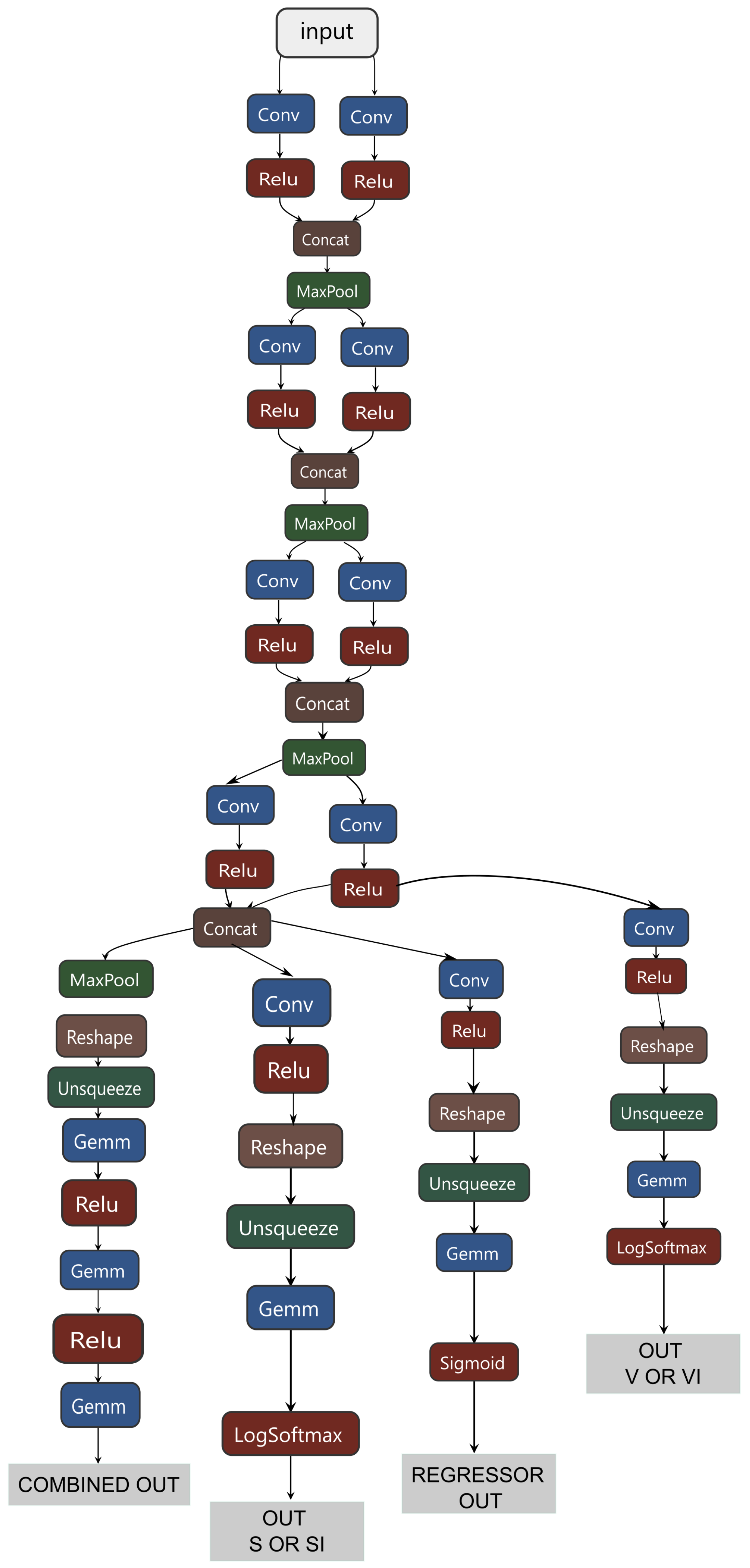
Thus, a hybrid classifier integrates several models, including a global classifier, two binary classifiers for processing SI and VI subclasses, and a regressor for processing the intermediate stage P. The general scheme of its structure is shown in Appendix A.1. Common information data were allocated for the SI subclass and the regression of class P, effectively identifying small and large predictors. Only large predictors were allocated for the VI subclass, proving to be the most effective approach.
The hybrid classifier’s training process involved several stages. First, only the global classifier was trained. Then, the binary classifiers and the regressor were trained, and the global classifier processed the input data. To train the global classifier, classes S and V included examples from both their samples and from classes SI and VI, respectively. In the next stage, binary classifiers S and V determined classes SI and VI.
The algorithm for determining the severity of intermediate AMD included a regressor operating in tandem with the Label Propagation (LPA) algorithm [57]. The training was conducted in three iterations using three different versions of the labeled dataset (1/6, 1/4, and 1/3). Accuracy was evaluated using a predetermined test dataset, which accounted for 10% of the total labeled data volume.
3. Results Obtained
Initially, a global classifier was trained to identify four main categories. The results of testing the global classifier are shown in the error matrix in Figure 4 and Table 3.
Testing of the global classifier revealed a significant reduction in class imbalance. It increased accuracy in P stage detection, suggesting that integrating the global classifier and regressor responses further improves the P detection process.
The values of the regressor were divided into three regions:
- P-free region (0–0,3);
- region of initial P progression (0,3–0,67);
- region of late P progression (0,67–1).
If the regressor’s response falls outside the first interval and the global classifier indicates that the class S closest to P is the correct one, then the final response is determined to be P.
In the next stage of developing a hybrid classifier, we trained binary classifiers to distinguish between the SI and VI classes. The results of testing these classifiers are illustrated as error matrices in Figure 5 and Figure 6, and their performance indicators are provided in Table 4.
The obtained data indicate that binary classifiers are effectively separate classes S and SI and V and VI, as the metrics show consistently high values even for adjacent classes.
The regressor was trained using a partially labeled data set, with 80% of the data used for training. The data set included three states: 0 - no P, 0.5 - the initial stage of P, and 1 - the extreme P stage. The Mean Absolute Error (MAE) and Root Mean Squared Error (RMSE) were used as metrics to evaluate the regression model. MAE calculates the average error in a set of forecasts and is less affected by outliers. On the other hand, RMSE calculates the square root of the average of the squared differences between the predicted and actual values. It is more sensitive to large deviations in the predicted value, allowing it to clearly emphasize significant discrepancies between the predicted and actual values [58].
First, the regressor was trained on these examples, and then the LPA model. The results of testing the regressor are presented in Table 5.
Concerning the boundaries we set for intermediate AMD progression, the outcome achieved using a 1/4 data set can be minimally acceptable. For subsequent work, we utilized a model trained on a data set with a 1/3 labeled data ratio.
The final stage of our study involved the comprehensive testing of the entire hybrid classifier. This testing was crucial in evaluating the performance of our system, and the results are presented in the error matrix in Figure 7 and Table 6.
Using Cohen’s Kappa coefficient, we assessed the agreement between the hybrid classifier and expert opinion, a statistical measure of their agreement [59]. The testing focused on diagnosing the most challenging cases of AMD, involving thorough analysis and comparison with an assessment scale. A set of 305 examples was given to an expert ophthalmologist, and the developed algorithm for evaluation. They were tasked with deciding whether to change the patient’s treatment plan after diagnosing the early stage of the disease during a prior examination. Cohen’s Kappa coefficient is calculated using the following formula:
where a is the number of times both test participants answered affirmatively; b is the number of times test participant 1 answered affirmatively and participant 2 answered negatively; c is the number of times test participant 1 answered negatively and participant 2 answered affirmatively; d is the number of times both test participants answered negatively; N is the total number of test examples.
During the testing of the algorithm and the expert, the following results were obtained:
Cohen’s kappa coefficient analysis shows a high agreement between expert assessments and the algorithm’s responses, demonstrating its effectiveness as a clinical decision-support tool.
The results indicate that the issues of class imbalance and complexity in identifying the intermediate stage of AMD have been effectively resolved. Additionally, the conservative classification for classes N and V has been minimized. This framework can be seamlessly integrated into the CDSS to help determine when to adjust a patient’s treatment plan. The hybrid classifier offers an accurate and interpretable assessment of the intermediate stage and early and late AMD outcomes.
4. Discussion
The developed hybrid classifier has demonstrated high efficiency and aligns well with expert assessments. However, it is essential to recognize that integrating the CDSS with the developed and trained CNN into medical practice may present several challenges. One significant issue is the need for more transparency regarding how the CNN arrives at clinical recommendations. The "black box" concept in hierarchical classification can lead to mistrust among diagnosticians, making it difficult to evaluate the system’s clinical significance. Future studies will focus on enhancing the transparency of CDSS for diagnosticians. It aims to build trust in the system and facilitate its integration into medical practice.
Moreover, the current study, while promising, is based on a limited dataset from a single clinical center. To truly gauge the generalizability of the classifier, it is imperative to work with a larger dataset that encompasses a wider range of OCT image sources and clinical pictures. This will be a key focus in our future studies.
In conclusion, this study demonstrates the possibility and potential of using the CDSS based on the hybrid classifier for monitoring changes in the management plan for patients with AMD. With further development and clinical validation, this system may simplify the treatment of AMD and enable earlier intervention, thereby improving the quality of healthcare services.
5. Conclusions
In this paper, we propose a hybrid approach for developing a CDSS to determine when to change the treatment plan for patients with AMD based on the analysis of OCT images. The architecture of our hybrid classifier consists of a global classifier, several local binary classifiers, and a regressor. The developed architecture effectively addresses class imbalance issues and accurately differentiates the intermediate stages of AMD, allowing for an assessment of its progression. By incorporating parallel convolutional layers with varying sizes of convolution kernels in the global classifier, the sensitivity of the CNN improved by at least 8%, and the harmonic mean also increased.
The class imbalance problem was addressed using hierarchical classification, which involved two binary classifiers in the architecture. In the subsequent transformation stage, these samples were closely correlated with the later stages of AMD. Modifications to the CNN resulted in high accuracy, sensitivity, specificity, and F1-scores exceeding 0.90 for all stages of AMD. This performance improvement surpassed the average value of the original four-layer encoder architecture by more than 20%. Additionally, the CNN structure included an algorithm designed to assess the severity of the intermediate stage of AMD. It includes a regressor that establishes the minimum ratio of labeled data to the entire dataset. This approach will aid in developing and modifying future hybrid algorithms for the CDSS. We calculated Cohen’s Kappa coefficient to evaluate the agreement between the algorithm’s results and expert assessments regarding the severity of the intermediate stage of AMD. The calculated value was 0.708, which indicates a remarkably high level of agreement between the algorithm and the experts’ evaluations.
Author Contributions
Conceptualization, L.E.; methodology, L.E. and Y.E.; software, L.E. and Y.E.; validation, I.R. and I.G.; formal analysis, I.G.; investigation, L.E., Y.E., I.R. and I.G.; resources, M.T., I.R. and I.G.; data curation, I.R. and I.G.; writing—original draft preparation, L.E.; writing—review and editing, L.E., G.E. and K.R.; visualization, L.E. and Y.E.; supervision, G.E. and I.G.; project administration, M.T. and K.R.; funding acquisition, G.E. and K.R. All authors have read and agreed to the published version of the manuscript.
Funding
The research is supported by the Ministry of Science and Higher Education of the Russian Federation within the state assignment for UUST (agreement № 075-03-2024-123/1 dated 15.02.2024) and conducted in the research laboratory "Sensor systems based on integrated photonics devices" of the Eurasian Scientific and Educational Center.
Institutional Review Board Statement
Not applicable.
Informed Consent Statement
Not applicable.
Conflicts of Interest
The authors declare no conflict of interest.
Abbreviations
The following abbreviations are used in this manuscript:
| AMD | Age-related Macular Degeneration |
| GA | Geographic Atrophy |
| MNV | Macular Neovascularization |
| SF | Subretinal Fibrosis |
| anti-VEGF | Intravitreal injections to inhibit the vascular endothelial growth factor |
| CV | Computer Vision |
| ML | Machine Learning |
| OCT | Optical Coherence Tomography |
| CDSS | Clinical Decision Support Systems |
| CNN | Convolutional Neural Networks |
| LPA | Label Propagation |
Appendix A
Appendix A.1. Structure of the Hybrid Classifier
Figure A1.
Figure caption.
References
- Stahl, A. The Diagnosis and Treatment of Age-Related Macular Degeneration. Deutsches Ärzteblatt international 2020. [Online; accessed 2024-09-13]. [CrossRef]
- Bressler, N.M. Antiangiogenic Approaches to Age-Related Macular Degeneration Today. Ophthalmology 2009, 116, S15–S23. [CrossRef]
- Yu, J.; Ba, J.; Peng, R.; Xu, D.; Li, Y.; Shi, H.; Wang, Q. Intravitreal anti-VEGF injections for treating wet age-related macular degeneration: a systematic review and meta-analysis. Drug Design, Development and Therapy 2015, p. 5397. [CrossRef]
- Lee, Y.; Ahn, E.J.; Hussain, A. Saponin-Mediated Rejuvenation of Bruch’s Membrane: A New Strategy for Intervention in Dry Age-Related Macular Degeneration (AMD). Recent Advances and New Perspectives in Managing Macular Degeneration 2022, pp. undefined–undefined. [CrossRef]
- Arrigo, A.; IRCCS San Raffaele Scientific Institute, Vita-Salute San Raffaele University, Milan, Italy.; Bandello, F.; IRCCS San Raffaele Scientific Institute, Vita-Salute San Raffaele University, Milan, Italy. Towards the Development of Longer and More Efficacious Therapies for Wet and Dry Age-related Macular Degeneration. US Ophthalmic Review 2022, 16, 30. [CrossRef]
- Wong, T.Y.; Lanzetta, P.; Bandello, F.; Eldem, B.; Navarro, R.; Lövestam Adrian, M.; Loewenstein, A. CURRENT CONCEPTS AND MODALITIES FOR MONITORING THE FELLOW EYE IN NEOVASCULAR AGE-RELATED MACULAR DEGENERATION: An Expert Panel Consensus. Retina 2020, 40, 1. [CrossRef]
- Ferris, F.L.; Wilkinson, C.; Bird, A.; Chakravarthy, U.; Chew, E.; Csaky, K.; Sadda, S.R. Clinical Classification of Age-related Macular Degeneration. Ophthalmology 2013, 120, 844–851. [CrossRef]
- Waugh, N.; Loveman, E.; Colquitt, J.; Royle, P.; Yeong, J.L.; Hoad, G.; Lois, N. Treatments for Dry Age-Related Macular Degeneration and Stargardt Disease: A Systematic Review. Health Technology Assessment 2018, 22, 1–168. [CrossRef]
- Garcia-Layana, A.; Cabrera-López, F.; García-Arumí, J.; Arias-Barquet, L.; Ruiz-Moreno, J.M. Early and intermediate age-related macular degeneration: update and clinical review. Clinical Interventions in Aging 2017, Volume 12, 1579–1587. [CrossRef]
- Morris, B.; Imrie, F.; Armbrecht, A.M.; Dhillon, B. Age-related macular degeneration and recent developments: new hope for old eyes? Postgraduate Medical Journal 2007, 83, 301–307. [CrossRef]
- LlorenteGonzález, S.; Hernandez, M.; GonzálezZamora, J.; BilbaoMalavé, V.; FernándezRobredo, P.; SaenzdeViteri, M.; BarrioBarrio, J.; RodríguezCid, M.J.; Donate, J.; Ascaso, F.J.; GómezRamírez, A.M.; Araiz, J.; Armadá, F.; RuizMoreno, Ó.; Recalde, S.; GarcíaLayana, A.; Spanish AMD group. The role of retinal fluid location in atrophy and fibrosis evolution of patients with neovascular agerelated macular degeneration longterm treated in real world. Acta Ophthalmologica 2022, 100. [Online; accessed 2024-06-21]. [CrossRef]
- Regillo, C.; Nijm, L.; Shechtman, D.; Kaiser, P.; Karpecki, P.; Ryan, E.; Ip, M.; Yeu, E.; Kim, T.; Rafieetary, M.; Donnenfeld, E. Considerations for the Identification and Management of Geographic Atrophy: Recommendations from an Expert Panel. Clinical Ophthalmology 2024, Volume 18, 325–335. [CrossRef]
- Zhang, J.; Sheng, X.; Ding, Q.; Wang, Y.; Zhao, J.; Zhang, J. Subretinal fibrosis secondary to neovascular age-related macular degeneration: mechanisms and potential therapeutic targets. Neural Regeneration Research 2025, 20, 378–393. [CrossRef]
- Fabre, M.; Mateo, L.; Lamaa, D.; Baillif, S.; Pagès, G.; Demange, L.; Ronco, C.; Benhida, R. Recent Advances in Age-Related Macular Degeneration Therapies. Molecules 2022, 27, 5089. [CrossRef]
- Lombardo, M.; Serrao, S.; Lombardo, G. Challenges in Age-Related Macular Degeneration: From Risk Factors to Novel Diagnostics and Prevention Strategies. Frontiers in Medicine 2022, 9. [CrossRef]
- Hagag, A.M.; Kaye, R.; Hoang, V.; Riedl, S.; Anders, P.; Stuart, B.; Traber, G.; Appenzeller-Herzog, C.; Schmidt-Erfurth, U.; Bogunovic, H.; Scholl, H.P.; Prevost, T.; Fritsche, L.; Rueckert, D.; Sivaprasad, S.; Lotery, A.J. Systematic review of prognostic factors associated with progression to late age-related macular degeneration: Pinnacle study report 2. Survey of Ophthalmology 2024, 69, 165–172. [CrossRef]
- Danzig, C.J.; Khanani, A.M.; Loewenstein, A. C5 inhibitor avacincaptad pegol treatment for geographic atrophy: A comprehensive review. Immunotherapy 2024, pp. 1–12. [CrossRef]
- Xu, Y.; Feng, Y.; Zou, R.; Yuan, F.; Yuan, Y. Silencing of YAP attenuates pericytemyofibroblast transition and subretinal fibrosis in experimental model of choroidal neovascularization. Cell Biology International 2022, 46, 1249–1263. [CrossRef]
- Ho, A.C.; Kleinman, D.M.; Lum, F.C.; Heier, J.S.; Lindstrom, R.L.; Orr, S.C.; Chang, G.C.; Smith, E.L.; Pollack, J.S. Baseline Visual Acuity at Wet AMD Diagnosis Predicts Long-Term Vision Outcomes: An Analysis of the IRIS Registry. Ophthalmic Surgery, Lasers and Imaging Retina 2020, 51, 633–639. [CrossRef]
- Shamsnajafabadi, H.; Daftarian, N.; Ahmadieh, H.; Soheili, Z.s. Pharmacologic Treatment of Wet Type Age-related Macular Degeneration; Current and Evolving Therapies. Archives of Iranian Medicine 2017, 20, 525–537.
- Flores, R.; Carneiro, Â.; Tenreiro, S.; Seabra, M.C. Retinal Progression Biomarkers of Early and Intermediate Age-Related Macular Degeneration. Life 2021, 12, 36. [CrossRef]
- Lad, E.M.; Finger, R.P.; Guymer, R. Biomarkers for the Progression of Intermediate Age-Related Macular Degeneration. Ophthalmology and Therapy 2023, 12, 2917–2941. [CrossRef]
- Boopathiraj, N.; Wagner, I.V.; Dorairaj, S.K.; Miller, D.D.; Stewart, M.W. Recent Updates on the Diagnosis and Management of Age-Related Macular Degeneration. Mayo Clinic Proceedings: Innovations, Quality & Outcomes 2024, 8, 364–374. [CrossRef]
- Sheeba, T.M.; Raj, S.A.A.; Anand, M. Computational Intelligent Techniques and Analysis on Automated Retinal Layer Segmentation and Detection of Retinal Diseases. 2023 9th International Conference on Advanced Computing and Communication Systems (ICACCS); IEEE, , 2023; pp. 2213–2219. [Online; accessed 2024-07-01]. [CrossRef]
- Koseoglu, N.D.; Grzybowski, A.; Liu, T.Y.A. Deep Learning Applications to Classification and Detection of Age-Related Macular Degeneration on Optical Coherence Tomography Imaging: A Review. Ophthalmology and Therapy 2023, 12, 2347–2359. [CrossRef]
- Burlina, P.M.; Joshi, N.; Pekala, M.; Pacheco, K.D.; Freund, D.E.; Bressler, N.M. Automated Grading of Age-Related Macular Degeneration From Color Fundus Images Using Deep Convolutional Neural Networks. JAMA Ophthalmology 2017, 135, 1170. [CrossRef]
- Leingang, O.; Riedl, S.; Mai, J.; Reiter, G.S.; Faustmann, G.; Fuchs, P.; Scholl, H.P.N.; Sivaprasad, S.; Rueckert, D.; Lotery, A.; Schmidt-Erfurth, U.; Bogunović, H. Automated deep learning-based AMD detection and staging in real-world OCT datasets (PINNACLE study report 5). Scientific Reports 2023, 13, 19545. publisher: Nature Publishing Group. [CrossRef]
- Tan, J.H.; Bhandary, S.V.; Sivaprasad, S.; Hagiwara, Y.; Bagchi, A.; Raghavendra, U.; Krishna Rao, A.; Raju, B.; Shetty, N.S.; Gertych, A.; Chua, K.C.; Acharya, U.R. Age-related Macular Degeneration detection using deep convolutional neural network. Future Generation Computer Systems 2018, 87, 127–135. [CrossRef]
- Govindaiah, A.; Hussain, M.A.; Smith, R.T.; Bhuiyan, A. Deep convolutional neural network based screening and assessment of age-related macular degeneration from fundus images. 2018 IEEE 15th International Symposium on Biomedical Imaging (ISBI 2018); IEEE, , 2018; pp. 1525–1528. [Online; accessed 2024-06-18]. [CrossRef]
- Abd El-Khalek, A.A.; Balaha, H.M.; Alghamdi, N.S.; Ghazal, M.; Khalil, A.T.; Abo-Elsoud, M.E.A.; El-Baz, A. A concentrated machine learning-based classification system for age-related macular degeneration (AMD) diagnosis using fundus images. Scientific Reports 2024, 14, 2434. [CrossRef]
- Bogunovic, H.; Montuoro, A.; Baratsits, M.; Karantonis, M.G.; Waldstein, S.M.; Schlanitz, F.; Schmidt-Erfurth, U. Machine Learning of the Progression of Intermediate Age-Related Macular Degeneration Based on OCT Imaging. Investigative Opthalmology & Visual Science 2017, 58, BIO141. [CrossRef]
- Yellapragada, B.; Hornhauer, S.; Snyder, K.; Yu, S.; Yiu, G. Unsupervised Deep Learning for Grading of Age-Related Macular Degeneration Using Retinal Fundus Images, 2020, [2010.11993]. [CrossRef]
- Yim, J.; Chopra, R.; Spitz, T.; Winkens, J.; Obika, A.; Kelly, C.; Askham, H.; Lukic, M.; Huemer, J.; Fasler, K.; Moraes, G.; Meyer, C.; Wilson, M.; Dixon, J.; Hughes, C.; Rees, G.; Khaw, P.T.; Karthikesalingam, A.; King, D.; Hassabis, D.; Suleyman, M.; Back, T.; Ledsam, J.R.; Keane, P.A.; De Fauw, J. Predicting conversion to wet age-related macular degeneration using deep learning. Nature Medicine 2020, 26, 892–899. [CrossRef]
- Liefers, B.; Taylor, P.; Alsaedi, A.; Bailey, C.; Balaskas, K.; Dhingra, N.; Egan, C.A.; Rodrigues, F.G.; Gonzalo, C.G.; Heeren, T.F.; Lotery, A.; Müller, P.L.; Olvera-Barrios, A.; Paul, B.; Schwartz, R.; Thomas, D.S.; Warwick, A.N.; Tufail, A.; Sánchez, C.I. Quantification of Key Retinal Features in Early and Late Age-Related Macular Degeneration Using Deep Learning. American Journal of Ophthalmology 2021, 226, 1–12. [CrossRef]
- Borrelli, E.; Serafino, S.; Ricardi, F.; Coletto, A.; Neri, G.; Olivieri, C.; Ulla, L.; Foti, C.; Marolo, P.; Toro, M.D.; Bandello, F.; Reibaldi, M. Deep Learning in Neovascular Age-Related Macular Degeneration. Medicina 2024, 60, 990. [CrossRef]
- Holland, R.; Kaye, R.; Hagag, A.M.; Leingang, O.; Taylor, T.R.; Bogunović, H.; Schmidt-Erfurth, U.; Scholl, H.P.; Rueckert, D.; Lotery, A.J.; Sivaprasad, S.; Menten, M.J. Deep Learning–Based Clustering of OCT Images for Biomarker Discovery in Age-Related Macular Degeneration (PINNACLE Study Report 4). Ophthalmology Science 2024, 4, 100543. [CrossRef]
- Yildirim, K.; Al-Nawaiseh, S.; Ehlers, S.; Schießer, L.; Storck, M.; Brix, T.; Eter, N.; Varghese, J. U-Net-Based Segmentation of Current Imaging Biomarkers in OCT-Scans of Patients with Age Related Macular Degeneration. Studies in health technology and informatics 2023, 302, 947–951. [CrossRef]
- Biloborodova, T.; Skarga-Bandurova, I.; Koverha, M.; Skarha-Bandurov, I.; Yevsieieva, Y. A Learning Framework for Medical Image-Based Intelligent Diagnosis from Imbalanced Datasets. Studies in Health Technology and Informatics 2021, 287, 13–17. [CrossRef]
- Prudhomme, C.; Schaffert, M.; Ponciano, J.J. Deep Learning Datasets Challenges For Semantic Segmentation -A Survey. Lecture Notes in Informatics, 2023.
- Yang, S.; Zhou, X.; Wang, J.; Xie, G.; Lv, C.; Gao, P.; Lv, B. Unsupervised Domain Adaptation for Cross-Device OCT Lesion Detection via Learning Adaptive Features. 2020 IEEE 17th International Symposium on Biomedical Imaging (ISBI); IEEE, , 2020; pp. 1570–1573. [Online; accessed 2024-09-13]. [CrossRef]
- Kim, W.; Kanezaki, A.; Tanaka, M. Unsupervised Learning of Image Segmentation Based on Differentiable Feature Clustering. IEEE Transactions on Image Processing 2020, 29, 8055–8068. [CrossRef]
- Brunekreef, J.; Marcus, E.; Sheombarsing, R.; Sonke, J.J.; Teuwen, J. Kandinsky Conformal Prediction: Efficient Calibration of Image Segmentation Algorithms, 2023, [arXiv:cs.CV/2311.11837].
- Orzeł, Z.; Kosior-Romanowska, A.; Bednarczuk, P. Methods of medical image segmentation analysis to improve the effectiveness of diagnosing lung diseases. Journal of Modern Science 2024, 57, 609–621. [CrossRef]
- Sajjadi, Z.; Esmaeili, M.; Ghobaei-Arani, M.; Minaei, B. A Hybrid Clustering Approach for link prediction in Heterogeneous Information Networks. Knowledge and Information Systems 2023, 65. [CrossRef]
- Mavaie, P.; Holder, L.; Skinner, M.K. Hybrid deep learning approach to improve classification of low-volume high-dimensional data. BMC Bioinformatics 2023, 24, 419. [CrossRef]
- Chou, Y.Y.; Shapiro, L.G. A hierarchical multiple classifier learning algorithm. Pattern Analysis & Applications 2003, 6, 150–168. [CrossRef]
- Silla, C.N.; Freitas, A.A. A survey of hierarchical classification across different application domains. Data Mining and Knowledge Discovery 2011, 22, 31–72. [CrossRef]
- Lin, Y.; Liu, H.; Zhao, H.; Hu, Q.; Zhu, X.; Wu, X. Hierarchical Feature Selection Based on Label Distribution Learning. IEEE Transactions on Knowledge and Data Engineering 2022, pp. 1–1. [CrossRef]
- Rezende, P.M.; Xavier, J.S.; Ascher, D.B.; Fernandes, G.R.; Pires, D.E.V. Evaluating hierarchical machine learning approaches to classify biological databases. Briefings in Bioinformatics 2022, 23, bbac216. [CrossRef]
- Qi, J.; Yang, H.; Kong, Z. A review of traditional image segmentation methods. 5th International Conference on Computer Information Science and Application Technology (CISAT 2022); Zhao, F., Ed.; SPIE, , 2022; p. 127. [Online; accessed 2024-06-25]. [CrossRef]
- Lindeberg, T. Scale-Space. In Wiley Encyclopedia of Computer Science and Engineering; John Wiley & Sons, 2009; pp. 2495–2504.
- Archana, R.; Jeevaraj, P.S.E. Deep learning models for digital image processing: a review. Artificial Intelligence Review 2024, 57, 11. [CrossRef]
- Zeng, S.; Zhao, Y.; Li, S. Comparison Between the Traditional and Deep Learning Algorithms on Image Matching. 2022 IEEE/ACIS 22nd International Conference on Computer and Information Science (ICIS); IEEE, , 2022; pp. 182–186. [Online; accessed 2024-06-25]. [CrossRef]
- Bria, A.; Marrocco, C.; Tortorella, F. Addressing class imbalance in deep learning for small lesion detection on medical images. Computers in Biology and Medicine 2020, 120, 103735. [CrossRef]
- Brigato, L.; Barz, B.; Iocchi, L.; Denzler, J. Image Classification With Small Datasets: Overview and Benchmark. IEEE Access 2022, 10, 49233–49250. [CrossRef]
- Jude Chukwura Obi. A comparative study of several classification metrics and their performances on data. World Journal of Advanced Engineering Technology and Sciences 2023, 8, 308–314. [CrossRef]
- Zhu, X.; Ghahramani, Z. Learning from labeled and unlabeled data with label propagation. School of Computer Science, Carnegie Mellon University, 2002.
- Hodson, T.O. Root-mean-square error (RMSE) or mean absolute error (MAE): when to use them or not. Geoscientific Model Development 2022, 15, 5481–5487. [CrossRef]
- Pacurari, A.C.; Bhattarai, S.; Muhammad, A.; Avram, C.; Mederle, A.O.; Rosca, O.; Bratosin, F.; Bogdan, I.; Fericean, R.M.; Biris, M.; Olaru, F.; Dumitru, C.; Tapalaga, G.; Mavrea, A. Diagnostic Accuracy of Machine Learning AI Architectures in Detection and Classification of Lung Cancer: A Systematic Review. Diagnostics 2023, 13, 2145. [CrossRef]
Figure 1.
Error matrix of the basic encoder model.
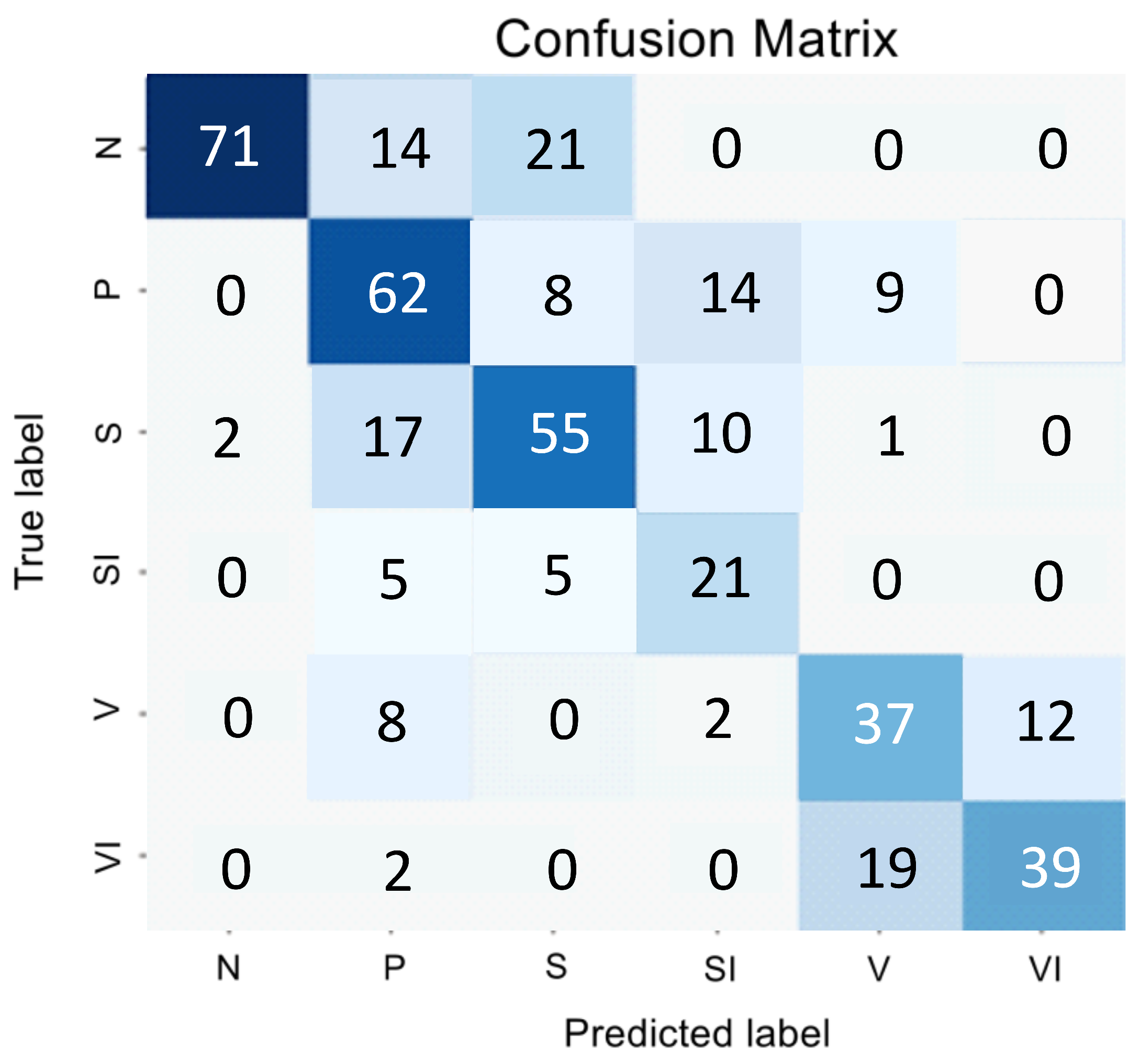
Figure 2.
Sensitivity of the model for classes S and V when using different sizes of convolution kernels.
Figure 2.
Sensitivity of the model for classes S and V when using different sizes of convolution kernels.
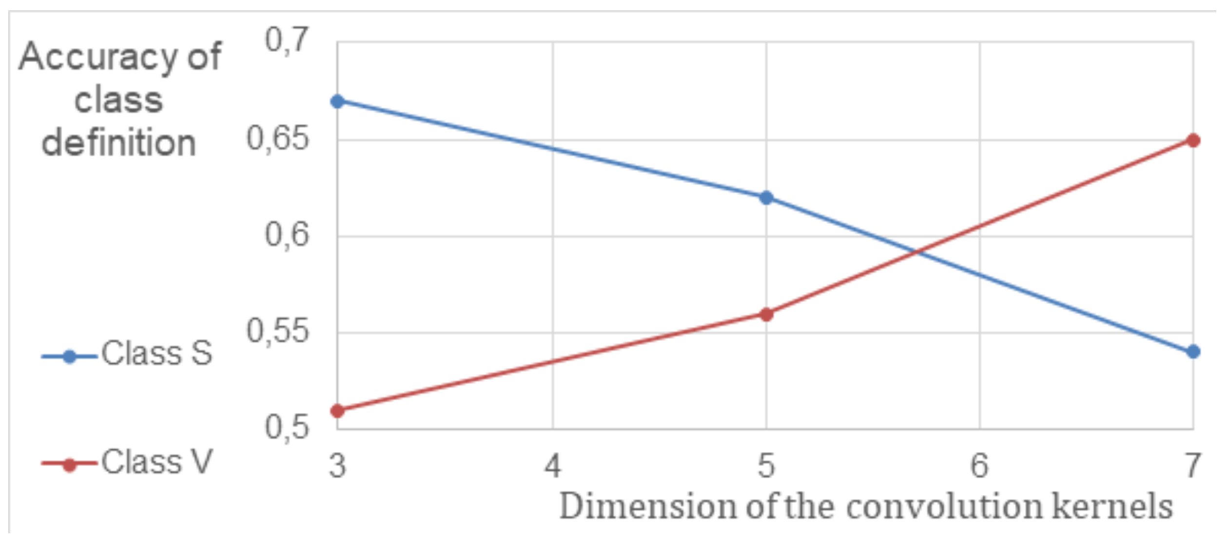
Figure 3.
Encoder error matrix with the inclusion of parallel convolutional layers in the architecture.
Figure 3.
Encoder error matrix with the inclusion of parallel convolutional layers in the architecture.
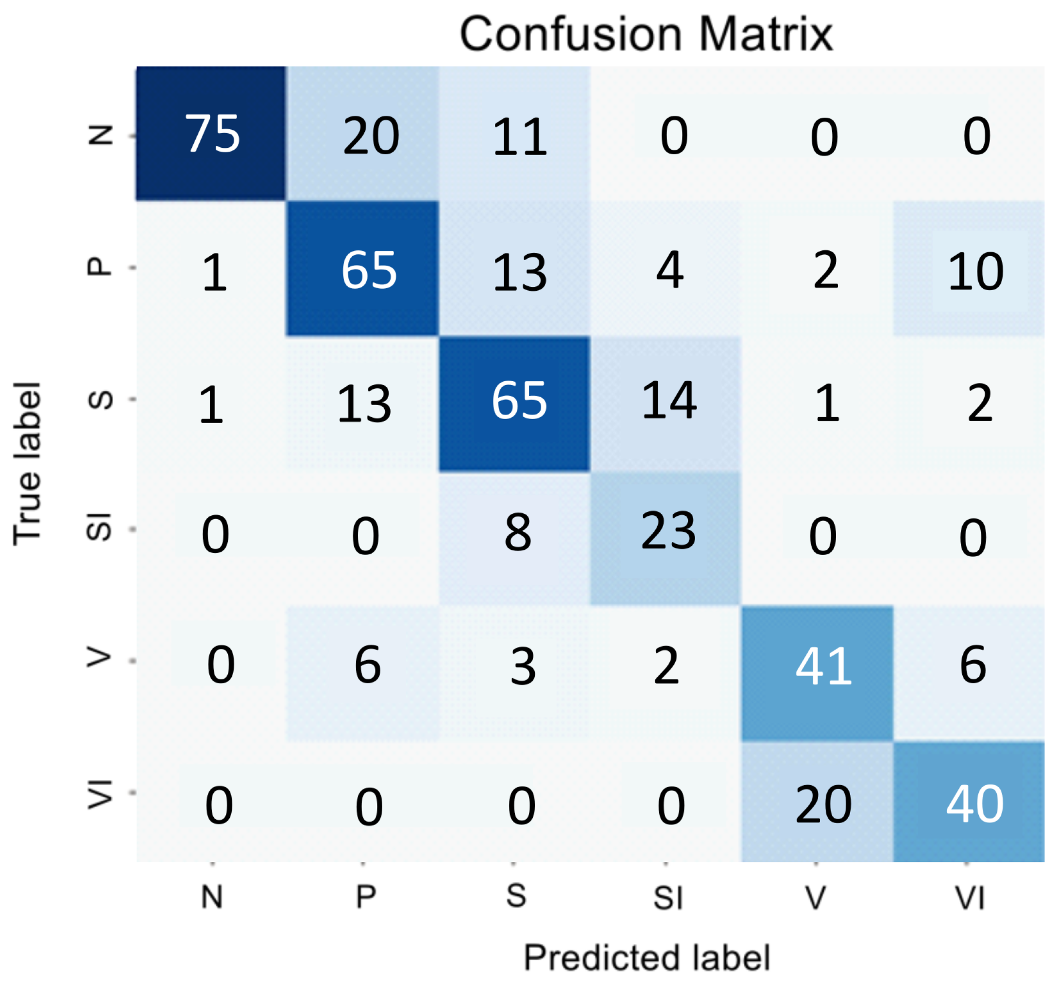
Figure 4.
Error matrix of the global classifier.

Figure 5.
Error matrices for binary classifier S and SI.

Figure 6.
Error matrices for binary classifier V and VI.
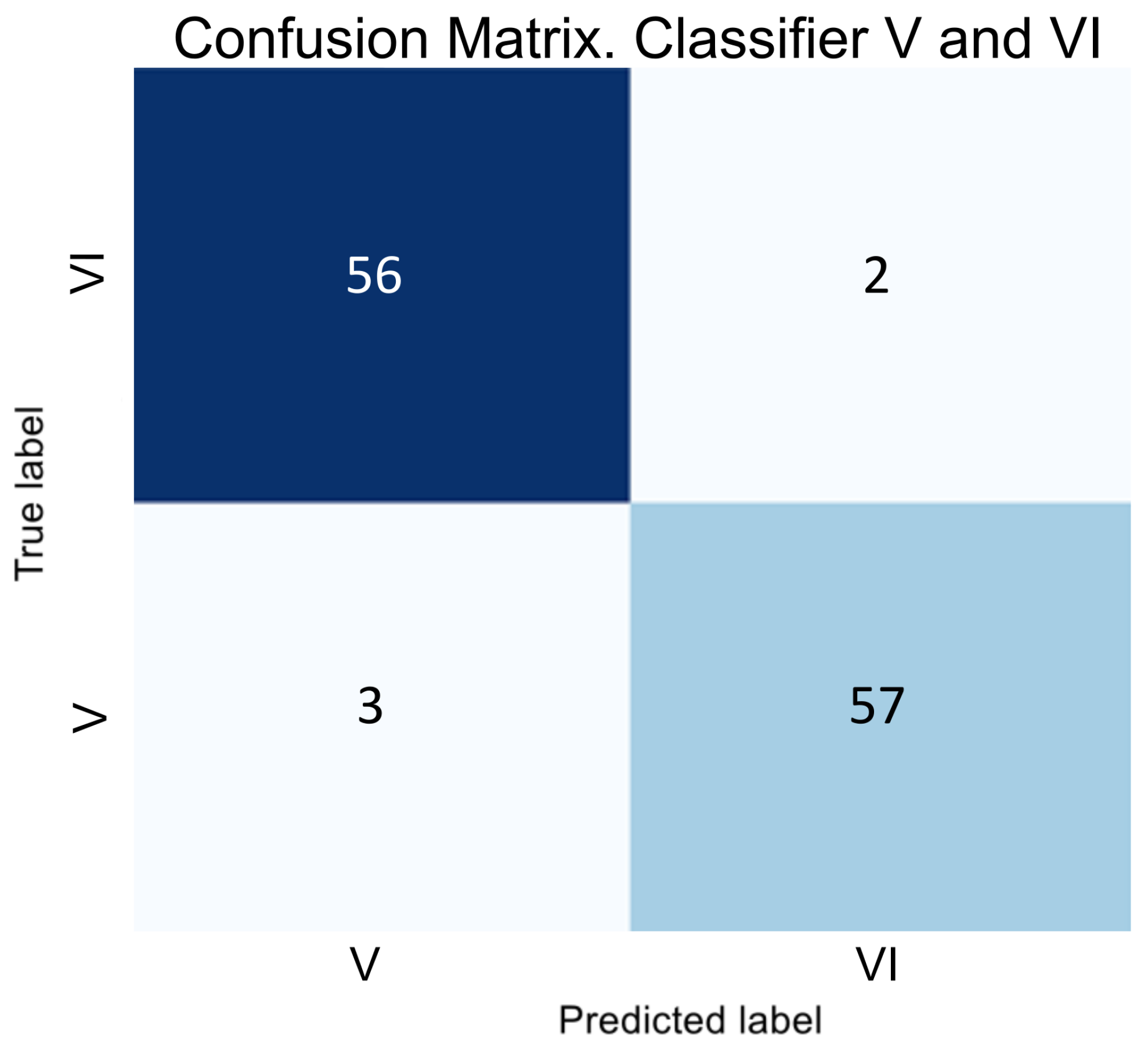
Figure 7.
Error matrix of hybrid classifier.
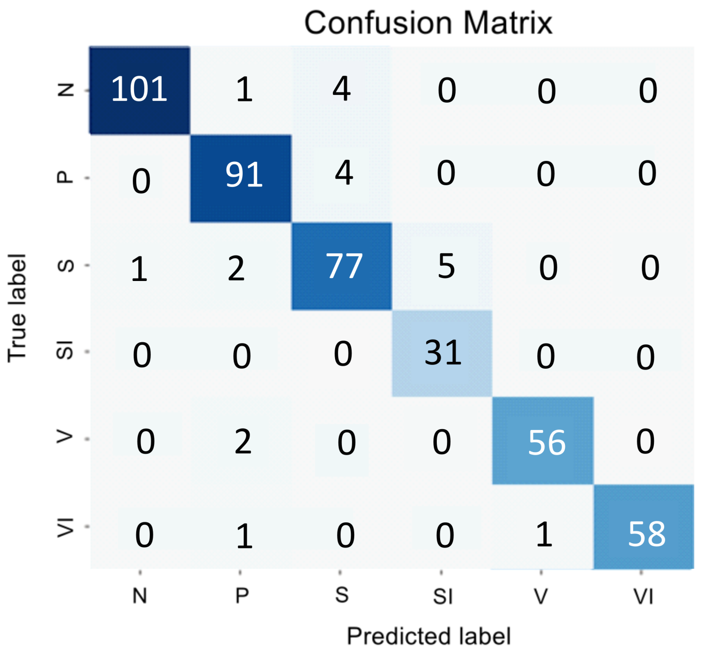

Table 1.
Performance indicators of the primary encoder model.
| Classes | N | P | S | SI | V | VI | |
|---|---|---|---|---|---|---|---|
| Metrics | |||||||
| Precision | 0.9725 | 0.5741 | 0.618 | 0.4565 | 0.5606 | 0.7358 | |
| Sensitivity | 0.6698 | 0.6526 | 0.6471 | 0.6774 | 0.6379 | 0.65 | |
| Specificity | 0.9939 | 0.8647 | 0.9029 | 0.9381 | 0.9231 | 0.9627 | |
| F1-score | 0.7933 | 0.6108 | 0.6322 | 0.5455 | 0.5968 | 0.6903 | |
Table 2.
Performance indicators of the primary encoder model with the inclusion of parallel convolutional layers in the architecture.
Table 2.
Performance indicators of the primary encoder model with the inclusion of parallel convolutional layers in the architecture.
| Classes | N | P | S | SI | V | VI | |
|---|---|---|---|---|---|---|---|
| Metrics | |||||||
| Precision | 0.974 | 0.6915 | 0.6465 | 0.5349 | 0.6406 | 0.6897 | |
| Sensitivity | 0.7075 | 0.6842 | 0.7529 | 0.7419 | 0.7069 | 0.6667 | |
| Specificity | 0.9939 | 0.9147 | 0.9 | 0.9505 | 0.939 | 0.952 | |
| F1-score | 0.8197 | 0.6878 | 0.6957 | 0.6216 | 0.6721 | 0.678 | |
Table 3.
Performance indicators of the global classifier.
| Classes | N | P | S | V | |
|---|---|---|---|---|---|
| Metrics | |||||
| Precision | 0.9182 | 0.7961 | 0.8350 | 0.9244 | |
| Sensitivity | 0.9528 | 0.8632 | 0.7414 | 0.9322 | |
| Specificity | 0.9726 | 0.9382 | 0.9467 | 0.9716 | |
| F1-score | 0.9352 | 0.8283 | 0.7854 | 0.9283 | |
Table 4.
Performance indicators of binary classifiers.
| Classes | S | SI | V | VI | |
|---|---|---|---|---|---|
| Metrics | |||||
| Precision | 0.9882 | 0.9677 | 0.9492 | 0.9661 | |
| Sensitivity | 0.9882 | 0.9677 | 0.9655 | 0.95 | |
| Specificity | 0.9677 | 0.9882 | 0.95 | 0.9655 | |
| F1-score | 0.9882 | 0.9677 | 0.9573 | 0.958 | |
Table 5.
Performance indicators of the regressor for assessing the degree of affinity between class P and classes S and V.
Table 5.
Performance indicators of the regressor for assessing the degree of affinity between class P and classes S and V.
| Markup percentage | 1/6 | 1/4 | 1/3 | |
| Metrics | ||||
| Mean Absolute Error | 0.2297 | 0.0882 | 0.0484 | |
| Root Mean Squared Error | 0.2827 | 0.1243 | 0.0551 | |
Table 6.
Performance of the primary encoder model with parallel convolutional layers included in the architecture.
Table 6.
Performance of the primary encoder model with parallel convolutional layers included in the architecture.
| Classes | N | P | S | SI | V | VI | |
|---|---|---|---|---|---|---|---|
| Metrics | |||||||
| Precision | 0.9902 | 0.9381 | 0.9059 | 0.8611 | 0.9825 | 1.00 | |
| Sensitivity | 0.9528 | 0.9579 | 0.9059 | 1.00 | 0.9655 | 0.9667 | |
| Specificity | 0.9970 | 0.9824 | 0.9771 | 0.9876 | 0.9973 | 1.00 | |
| F1-score | 0.9712 | 0.9479 | 0.9059 | 0.9254 | 0.9739 | 0.9831 | |
Disclaimer/Publisher’s Note: The statements, opinions and data contained in all publications are solely those of the individual author(s) and contributor(s) and not of MDPI and/or the editor(s). MDPI and/or the editor(s) disclaim responsibility for any injury to people or property resulting from any ideas, methods, instructions or products referred to in the content. |
© 2024 by the authors. Licensee MDPI, Basel, Switzerland. This article is an open access article distributed under the terms and conditions of the Creative Commons Attribution (CC BY) license (http://creativecommons.org/licenses/by/4.0/).
Copyright: This open access article is published under a Creative Commons CC BY 4.0 license, which permit the free download, distribution, and reuse, provided that the author and preprint are cited in any reuse.


