Bone Fracture Detection from X-ray Images using a Convolutional Neural Network (CNN)

Sultan Mamun; Md Al Amin; Ajlan Jamal Ali; Jingwei Li

doi:10.20944/preprints202410.1320.v1

Submitted:

15 October 2024

Posted:

16 October 2024

You are already at the latest version

Abstract

Bone fractures are common injuries that require quick and accurate diagnosis to provide the right medical care. The “convolutional neural network” technique relies mostly on manual inspection, by radiologists and can be laborious and prone to error. The objective of this work was to increase the efficiency and accuracy of fracture identification by automating the examination of X-ray images using convolutional neural networks. A “convolutional neural network” model created to detect bone fractures in X-ray images was used in the present study. The model was trained and validated using an extensive dataset of X-ray images, which included both fractured and nonfractured bones. Multiple convolutional layers were used in the “convolutional neural network” architecture for feature extraction, and pooling and fully connected layers were added for classification. The main measures used to assess the model's performance were sensitivity, specificity, and accuracy. In regard to identifying bone fractures, the “convolutional neural network”-based model outperformed the conventional technique. With significant gains in sensitivity and specificity, this approach achieved a high accuracy rate and decreased the frequency of false positives and false negatives. We used “convolutional neural network” tool in PyTorch for bone fracture detection and we outlined the important considerations that must be considered when attempting to achieve this goal Additionally, we contrasted every study with our baseline. Here our maximum accuracies were 99.05%, 98.60%, 99.45% and 99.74% for epochs 8, 9, 10 and 11, respectively. These findings highlight the model's ability to improve the diagnostic efficiency and accuracy in clinical settings. Using “convolutional neural network” to identify bone fractures from X-ray images is a promising development in medical imaging. In the end, our method improves patient outcomes by ensuring faster and more reliable fracture diagnosis while also lessening the diagnostic burden on radiologists. Subsequent investigations will focus on incorporating this system into clinical procedures and investigating its utilization in real-time emergency situations. Since there was no medical intervention on human subjects in this investigation, trial registration regulations were not applied.

Keywords:

X-ray image

;

Convolutional neural network

;

Bone fracture

;

Python

;

PyTorch

Subject:

Engineering - Electrical and Electronic Engineering

I. Introduction

Bone fracture is a currently one of the most common injuries. It is a global public health issue. Every year more bone fractures occur in China, Bangladesh, India, Pakistan and other regions. Globally millions of people suffer from bone fracture every year. Only in the United States are millions of bone fractures found every year [1]. By employing CNNs for experimental bone fracture detection, medical imaging and machine learning research has advanced, and patient care may be enhanced by precise and effective fracture detection. A great responsibility for this lies with the doctors, who must evaluate tens of X-ray images a day. The majority of the technology used for initial diagnosis is X-ray technology, which has been used for more than a century and is still widely employed. Examining X-ray images can be difficult for physicians for three reasons: first, the images may obscure certain characteristics of the bone; second, the classification of fractures requires extensive experience; and third, physicians frequently respond to emergency cases and may be fatigued. In fact, research indicates that radiologists perform worse toward the end of the workday than they did at the start in regard to fracture detection while interpreting musculoskeletal radiographs. Furthermore, radiographic interpretation frequently occurs in settings without access to trained peers.

A precise classification of fractures among standard forms is critical for ensuring good prognosis and therapeutic efficacy. In this situation, a computer-aided diagnosis system that supports physicians could directly affect the way patients progress. We covered a number of topics in this work, ranging from fundamental strategies to the most important sophisticated fixes. Convolutional neural network operations, which include preprocessing, feature extraction, and classification steps, were the focus of early earlier efforts in the detection and classification of fractures. Bone fracture detection using CNN techniques has recently produced remarkable results. Through database searches and other sources, additional records were found. Following a screening and exclusion process for all records, the eligibility of the full-text publications was evaluated. We chose records from these papers for analysis. Only a small number of them attempted to categorize the various forms of fractures, but the majority focused on distinguishing between bones that were broken and those that were not. We selected studies that, in our opinion, best demonstrated the advantages of a CNN detection technique for the development of a universal tool capable of categorizing all forms of fractures in the body’s bones.

II. Related Work

One of the earliest and most widely used diagnostic techniques in clinical medicine is X-ray, which can produce images of any bone, including the hand, wrist, hip, pelvis etc [1]. Fractures are a common bone disease that arise when a bone is unable to tolerate external forces such as direct blows. falls or twisting injuries [2]. Bone cracks known as fractures are described as medical conditions in which the bone's continuity of the bone is disrepute [2]. Finding fractures and treating them properly are seen as significant since an incorrect diagnosis frequently results in ineffective patient care, a rise in complaints, and costly legal action Bone fracture detection is a difficult task, particularly in the presence of sound. There are several differences between PECTS and conventional object detection including the following. 1. The scales of different bones vary greatly on X-ray images [3]. The human bone structure diagram shows various bone types, including the wrist, radius, skull, and so forth. 2. Different fracture types, such as traverse, open, simple, spiral, and comminuted fractures, have distinct textures and shapes. As a result, identifying bone fractures in various bone types is crucial [4].

The majority of early research on bone fracture detection focused on employing computer graphics and machine learning to identify fractures in particular bone regions [5]. As previously mentioned, they extracted features from pelvic CT scans using wavelet transform, adaptive windowing, and boundary tracing. A registered active shape model was subsequently used to identify fractures.

To identify fractures in X-ray images, Yu et al. [6] employed stacked random forests based on feature fusion. Multiple classifiers, including the Back Propagation Neural Network, K-Nearest Neighbor, Support Vector Machine, Max/Min Rule, and Product Rule, are fused to design as a combined classifier to detect fractures after edge and shape features are extracted from bone [7,8]. Among other things, bone fracture detection has made extensive use of mathematical morphology [9]. These techniques can identify whether an image is fractured based on the entire picture [3,5,9], but they are unable to identify the specific bone region that is broken. An entropy-based thresholding method was employed in earlier work to separate the surrounding flesh region from a bone region in X-ray images. Numerous individuals notice a break in a single human bone. The authors of Ref. [10] proposed an automated fracture detection system that relies on filtering algorithms to eliminate noise, edge detection techniques to identify edges, wavelet and curvelet transforms to extract features, and the construction of decision tree-style classification algorithms in hand bones using X-ray images. An algorithm based on the grey level cooccurrence matrix (GLCM) was presented by Chai et al. [11] to identify femur fractures, if any were present. Additionally, in Reference [12], the authors identified femur fractures by extracting the femur contour using a modified Canny edge detection algorithm, calculating the neck-shaft angle from the femur contour, and utilizing the neck-shaft angle to construct classification algorithms. The authors of Ref. [12] preprocessed X-ray/CT images using techniques such as segmentation, edge detection, and feature extraction. They then used a variety of classifiers, including decision trees (DTs), neural networks (NNs), and meta-classifiers, to classify fractured and nonfractured images, with an excellent accuracy of 85% on 40 images. To facilitate easy visualization of the fracture [5] combined an entropy-based segmentation method with an adaptive thresholding-based contour tracing technique to localize the line-of-break, identify its orientation, and evaluate the degree of bone damage surrounding a long-bone digital X-ray image. A fusion classification technique was proposed by Mahendran and Baboo [13] for the automatic detection of fractures in the tibia bone, one of the long bones of the leg. Deep convolutional networks were used in another study [1] to automatically detect posterior element fractures in the spine using CT scans.

These techniques can only identify fractures in medical images of a single bone [1,5,11,12,13]. Fractures cannot be identified in images of other types of bones in the human body to aid medical professionals in identifying fractures, but we have used different bone X-ray images from the human body. They used a traditional method of using genetic algorithms [13] and Canny edge detectors [12] to segment pictures for medical purposes. Additionally, they employed 2D and 3D CNNs for MR structural image segmentation via automatic proximal femur segmentation. These techniques, however, were unable to distinguish between various bone types.

III. Methods

Convolutional neural networks (CNNs) are built using PyTorch and require a number of steps to be completed, including system architecture and data preparation, model architecture definition, training, and evaluation. We take the following general approach. This is our basic outline, and we need to adapt it to our specific requirements and dataset characteristics. Experimentation and iteration are key to finding the best model for the task.

A. System Architecture

A variety of bone X-ray images were obtained, including examples of both healthy and broken bones. The photos were preprocessed to normalize the pixel values, adjust the contrast, and standardize the size. The training, validation, and test sets were constructed from the dataset. This guarantees that the model learns from a single set of data and makes good generalizations to new data. Utilizing the training dataset, the CNN model is trained. This entails feeding the network images, optimizing the model with an appropriate loss function, and modifying the model’s weights through backpropagation.

To ensure that the trained model did not overfit the training set, we validated it using the validation set. As necessary, adjust the hyperparameters. The model’s generalization performance was analyzed using the test set. Postprocessing techniques，such as thresholding, are used to enhance accuracy and refine the model’s output. This approach could be implemented as part of a web application, in a hospital setting, or integrated with a picture archiving and communication system [12,13].

B. Model Architecture

The sizes of the input layer and previously processed images should match. To capture hierarchical features in images, multiple convolutional layers are stacked. To find distinct patterns, filters of different sizes were used. To enable the model to learn complex relationships, nonlinearity is introduced after each convolutional layer using activation functions such as rectified linear unit.

Figure 1. Model Architecture.

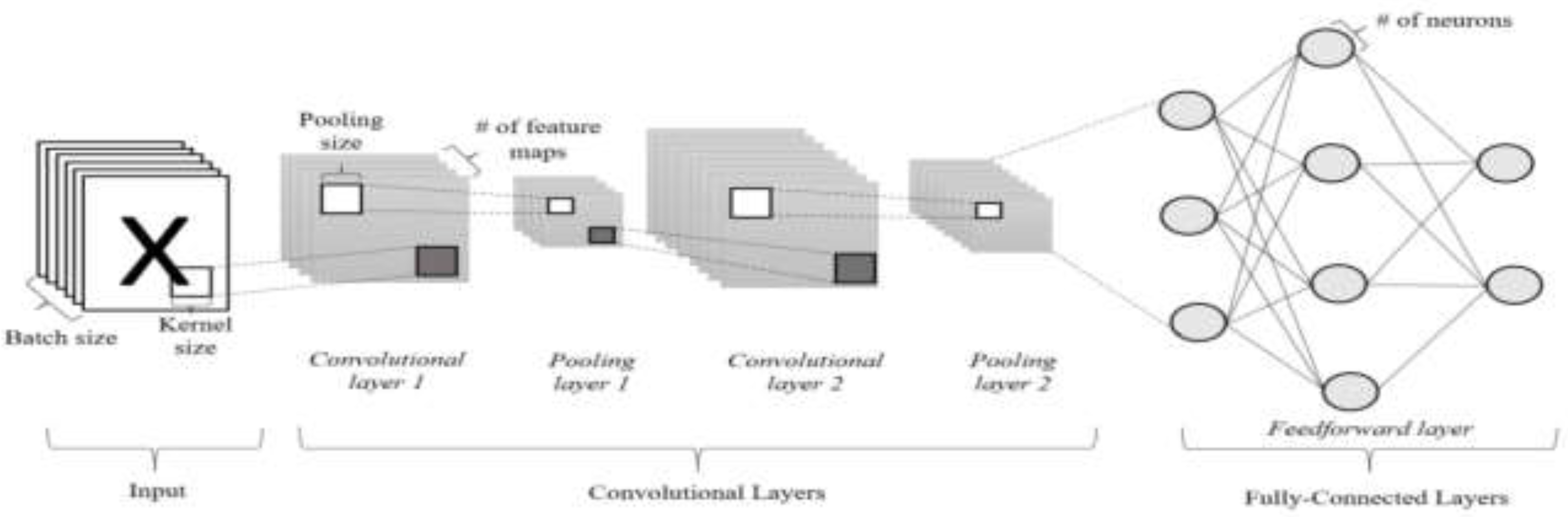
To decrease the computational load and down sample the spatial dimensions, pooling layers (such as max pooling) are added. The convolutional layer output should be flattened into a vector so that it can be fed into the dense, fully connected layers. One or more dense layers are added to the model for classification. These layers process the extracted features and determine whether a fracture is present. The output layer should have the same number of neurons as the other classes (normal or fractured). For binary classification, a SoftMax activation function is used. A suitable loss function such as binary cross-entropy loss is selected for binary classification tasks [16,17]. The robustness and generalizability of a convolutional neural network (CNN) model can be evaluated by comparing it to a more difficult dataset when evaluating a bone fracture detection model. Suitable metrics such as the F1-Score, specificity, accuracy, precision, recall or sensitivity, area under the receiver operating characteristic curve (AUC-ROC), are chosen for assessment [18].

The selected performance metrics were determined, and the trained model was assessed using the test set. Classification reports and confusion matrices are created to learn more about the model’s performance for various fracture types. Display ROC curves, precision-recall curves, and examples of correctly and incorrectly classified images using visualization tools.

If the model’s performance does not reach par, implement regularization strategies such as dropout or L1/L2 regularization, modify hyperparameters, or fine tune the architecture [19]. Examine how well the model performs on the difficult dataset in comparison to a standard dataset. This approach enables one to determine whether the accuracy of the model decreases noticeably in more complicated cases [20].

IV. Experiment

This experiment aimed to assess how well a convolutional neural network (CNN) performs in detecting bone fractures using various configurations of hyperparameters, particularly epochs and learning rates. We used a specific MURA dataset from different sources. We obtained 9193 images for training and 8907 images for testing. There are multiple phases involved in building a convolutional neural network (CNN) with PyTorch for bone fracture diagnosis. We have modified this term in accordance with the dataset and needs. Here we assume that the dataset of bone X-ray images is arranged into folders for each class (fracture or no fracture):

We imported our necessary libraries. The CNN model was defined as necessary. We change the filter sizes, fully connected layer sizes, and number of channels and input the dimensions. In addition, depending on the intricacy of the dataset, batch normalization or dropout layers are incorporated for regularization. We then organized and split the dataset into training and testing sets. We used an image folder for image classification tasks and put the dataset into folders with distinct „fracture” and „no fracture” subfolders for each class. We used transforms to apply data transformations to resize, normalize and enhance the images then we used compose. We ensure that, the path to the dataset is substituted for „/path/to/dataset”. Finally, during the training and testing stages, the CNN model can loop through batches of data using these data loaders. This is our fundamental training cycle to include more advanced features such as learning rate scheduling, early stopping, or model checkpointing, depending on my particular use case. The learning rate and number of epochs are two examples of hyperparameters that can be adjusted based on how well the model performs and converges on training and test sets.

Figure 2. Fracture Detection/ Fracture Image.

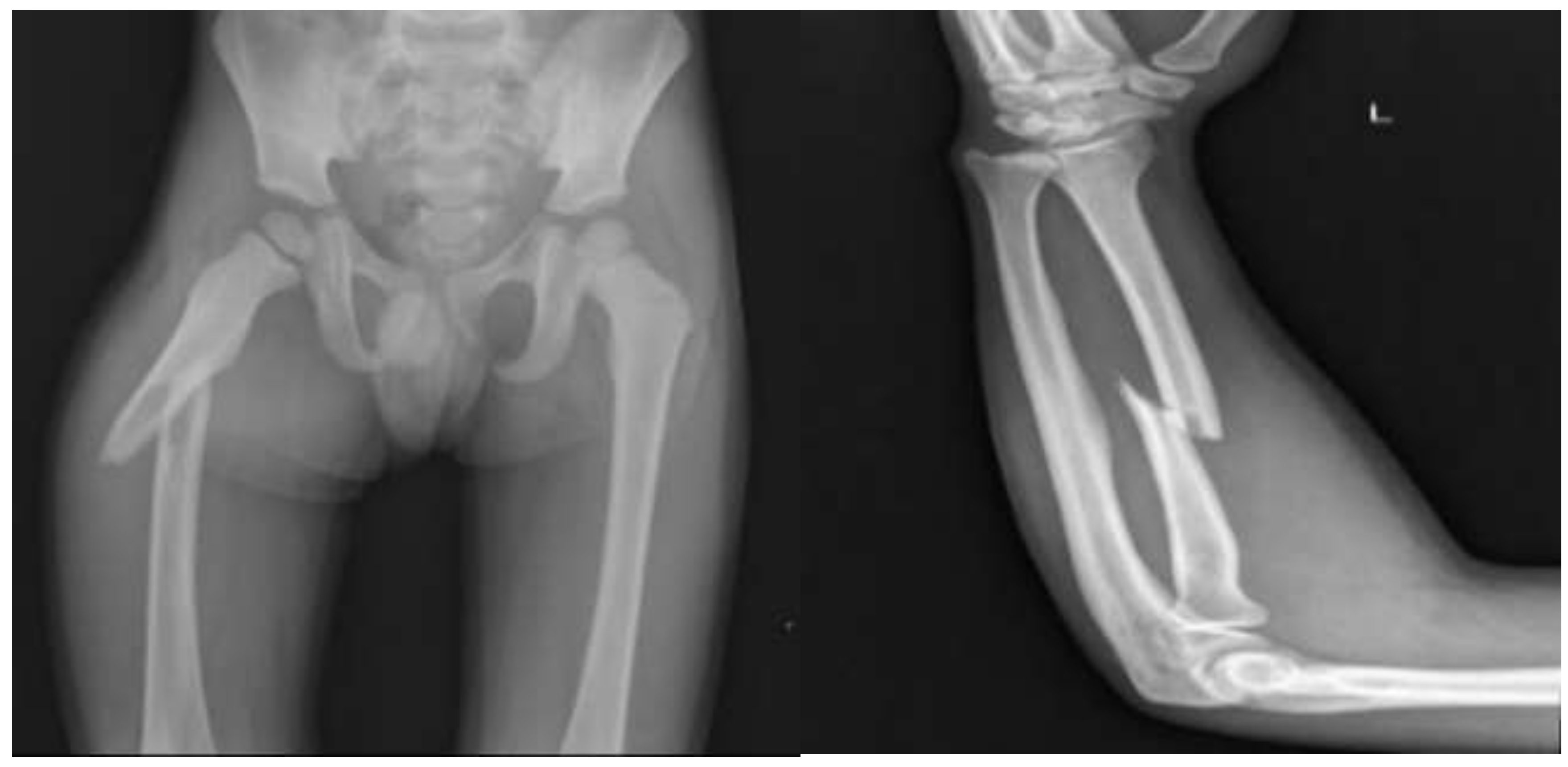
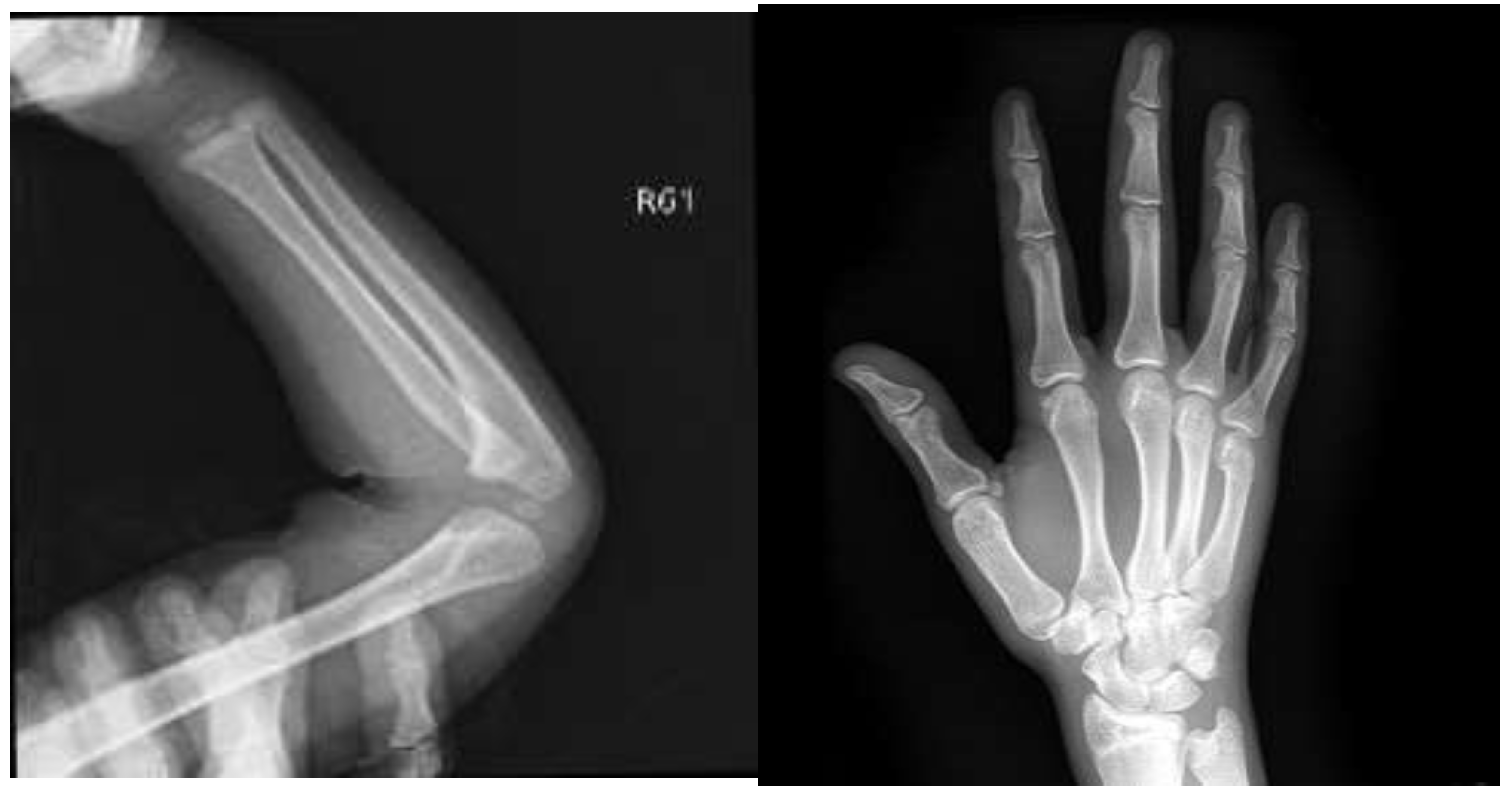
Figure 3. No Fracture Detection/ Non-Fracture Images.

We analyzed our model with fresh data after training, and adjusted the hyperparameters as necessary. This simple template needs to modified depending on the requirements, model architecture, and particular dataset to further enhance the performance, of the algorithm, taking into account learning rate scheduling, data augmentation, and other methods. The CNN architecture is depends on the unique requirements and characteristics of the dataset, the architecture, hyperparameters, and data preprocessing steps need to be modified. To monitor the model’s performance during training and avoid overfitting, we should also divide the data into training and validation sets. The CNN model’s ability to detect bone fractures can be largely impacted by the selection of hyperparameters, especially learning rates and epoch counts. To find the hyperparameter combinations that produce the best results in terms of accuracy, generalization, and convergence, experimentation is necessary.

CNN from scratch in PyTorch training. Here the CNN network uses different layers. Training the CNN with the dataset and saving the best model based on testing accuracy. We arranged the datasets, and the data sets contain 9193 training and 8907 test images of size 150*150 distributed into two categories: fracture images and nonfracture images. For the first step we imported the all-necessary libraries. Then they are used to transform and process the data. First all the images were resized to 150 heights and 150 widths. Then I used the transform to tensor, which changed the picture of each color channel from 0-255 to 0-1. This process change the data type NumPy to tensors. Then “transform. Normalized” changes the range from 0-1 to [-1,1]. Here the data loader helps readers read the data and gates the model for training in batches. Additionally, the batch size should be adjusted according to the GPU or CPU memory. A higher batch size cannot lead to memory overload which can load to an error. Paths for training and testing directories both have holders for the categories and need to classified with images inside them. In the next steps all the classes are fetched.

Here the CNN network class extends the “nn.Module”. The class specifies the entire layers network. Before the start of the network, the shape of the image batch is (256,3,150,150), the height is 150, and the widths of the image is 150. Therefore, the formula for the height and width of the CNN output is ((w-f+2p)/s) +1. Here the training accuracy was 0.995, and the test Accuracy was 0.994.

V. Results

Table 1. various results for training AND testing statistics.

Epoch	Train Loss	Train Accuracy	Test Accuracy
0	3.3721	0.62841292	0.74952284
1	0.4713	0.81388012	0.90917256
2	0.4813	0.830523224	0.813292915
3	0.4554	0.849559447	0.948018412
4	0.1532	0.94528445	0.97799483
5	0.0916	0.973022952	0.981250701
6	0.0580	0.984009572	0.991018300
7	0.0573	0.98455346	0.99404962
8	0.0409	0.990536277	0.977658021
9	0.0484	0.98607636	0.99056921
10	0.0263	0.99456107	0.99607050
11	0.0188	0.99749809	0.99517233
12	0.0176	0.99738931	0.99640732
13	0.0155	0.99793321	0.99793321

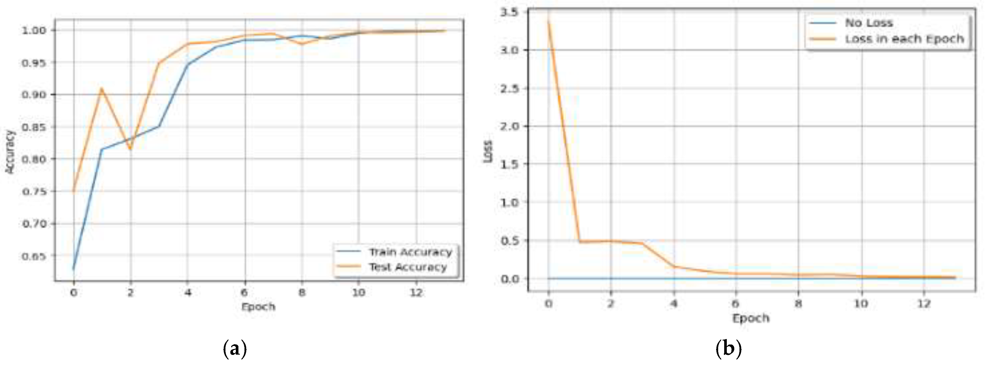
Various hyperparameters can influence the learning process and, ultimately, the loss versus epoch curve when training a convolutional neural network (CNN) from scratch. The best hyperparameters can vary depending on the dataset and problem at hand. Experimentation and hyperparameter tuning are frequently required to find the optimal set of hyperparameters for a CNN. It is critical to monitor the loss versus epoch curve and validation performance during this process to ensure that the model converges effectively and avoids overfitting.

Figure 4. Results for 8 Epochs.

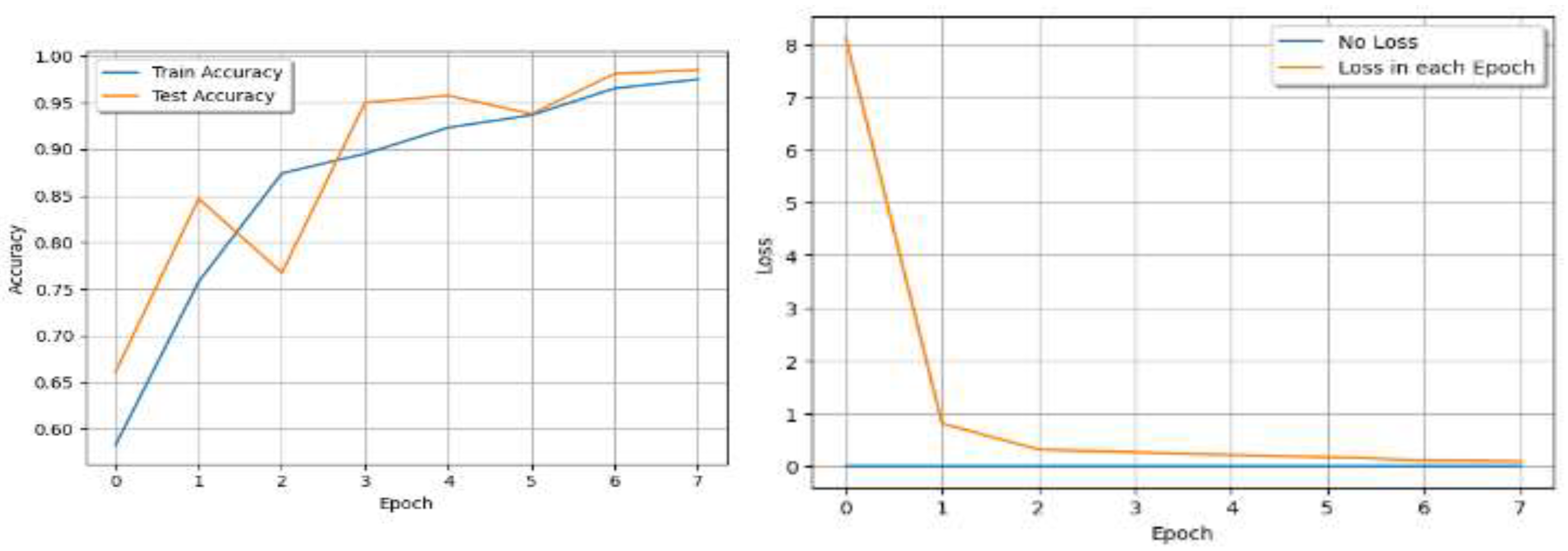
Figure 5. Results for 14 Epochs.

VI. Discussion

When the number of epochs changes from a small to a high number, the increase in accuracy also decreases the loss. Higher learning rates may lead to faster convergence but risk overshooting the optimal weights. This can result in a loss curve that exhibits oscillations or fails to converge. Lower learning rates are more stable but may require longer training times for convergence. The loss curve tends to decrease gradually. A more irregular loss curve and noisy updates can result from a smaller batch size. However, this approach can aid in the model’s escape from local minima. A smoother loss curve and more stable gradients can be obtained with a larger batch size. However, if the batch size is too large, more memory might be needed, possibly leading to convergence problems. Insufficient epochs of training could lead to an underfit model with an early plateauing loss curve. Overfitting, in which the loss in the validation set begins to increase while the training loss continues to decrease, can result from training for an excessive number of epochs. The loss curve’s shape can be affected by the use of learning rate schedules, such as cyclic learning rates or learning rate decay. During training, these schedules modify the learning rate.

VII. Compared with the Other Results

A comparison of ‘Table 2’ with ‘Veerabhadra Rao Marellapudi’s paper name- ‘Building and Training a Custom Convolutional Neural Network with PyTorch’ yielded maximum accuracies of 61.18%, 61.88%, 62.05% and 62.75% for epochs 8, 9, 10, 11, respectively. However, in our study, the maximum accuracies were 99.05%, 98.60%, 99.45% and 99.74% for epochs 8, 9, 10, 11 respectively. Additionally, at the same epochs the training loss was 0.8948, 0.8859, 0.8875 and 0.8824 and at the same epochs our training loss was 0.0409, 0.0484, 0.0263 and 0.0188- [14].

A comparison of ‘Table 3’ with the paper name- Bone Fracture Detection in X-ray Images using a Convolutional Network yielded maximum accuracies of 87.20%, 86.82%, 88.00% and 89.90% for epochs 10, 20, 20, 20 respectively. However, in our study, the maximum accuracies were 99.05%, 98.60%, 99.45%, and 99.74% for epochs 8, 9, 10, 11 respectively [15].

Figure 6 and Figure 7 show the changes in accuracy and validation accuracy while training the model. The accuracy of the training data was 95.0%, and the accuracy of the test data was 69.4%. was 96.6%, 89.7%, and 98.2%, respectively. For the test data, the precision, recall, and specificity were 60.0%, 60.4%, and 75.0%, respectively [16]. However, in our study, the maximum accuracy 99.05%, 98.60%, 99.45%, and 99.74%, and the maximum accuracies was 0.996, 0.995, 0.996, and 0.997 for epochs 8, 9, 10, and 11respectively. A comparison of the above results with those of others related studies revealed that, in our work, the test and training accuracies were better than the minimum loss. We have taken different epochs, and models and illustrated more results to increase the learning rate and accuracy.

VIII. Description of Shortcomings and Improvements

A significant drawback of a convolutional neural network (CNN) model for bone fracture detection from X-ray images is its limited generalization capacity. However CNN models may find it difficult to reliably distinguish fractures, such as rare fracture patterns, different imaging characteristics, or particular patient demographics, in X-ray images from cases that have never been previously observed. This is because the model is not able to learn and generalize well on diverse and uncommon scenarios that were not comprehensively represented in the training data. A representative and diverse training dataset covering a broad range of fracture types, patient demographics, and imaging characteristics is essential for addressing the generalization problem. Obtaining a large number of samples from a comprehensive dataset can aid in the model’s learning of resilient features and patterns. [21]

The CNN model can acquire low-level features more successfully if it is pretrained on a sizable dataset from a related domain, such as generic X-ray images or medical images. The particular dataset was used to fine-tune the pretrained model on the bone fracture detection task. Through transfer learning, the model’s performance can be enhanced by utilizing information from larger datasets and tailoring it to the particular task at hand [23]. To prevent bias toward the majority class, the dataset was balanced across various fracture types. Reducing class imbalance can improve the model’s ability to identify uncommon fracture patterns [24]. To integrate several trained CNN models, ensemble techniques such as model averaging or bagging are used. By utilizing the advantages of several individual models and mitigating the effects of their shortcomings, ensemble learning can enhance the performance of the model [23]. To avoid overfitting and improve the model’s capacity to generalize well to unknown data, regularization techniques such as weight decay or dropout are incorporated [25]. Medical specialist input the data, and the model’s performance on fresh data was continuously assessed. The required iterative improvements are achieved by utilizing this feedback to pinpoint and resolve model limitations [24].

IX. Conclusion

Given the labelled training and validation images, the problem statement aimed to investigate the classification accuracy of various supervised and unsupervised models for different Heri X-ray images: normative vs. anomalous (anomalous being humeri that are broken, fractured, or have implants). To feed the normalized histograms of each image into the supervised learning algorithms, we preprocessed the images. In contrast to our initial expectation, “convolutional neural network” would perform best.

We used a variety of datasets for fracture detection and classification in this paper. Fracture detection techniques can be used to automate the labor-intensive and time-consuming process of expert radiologists diagnosing and interpreting radiographs. Many of the researchers cited state that the biggest obstacle to creating a high-performance classification algorithm is the lack of labeled training data. Currently, no industry-standard model exists that can be applied to the available data. We have made an effort to demonstrate how deep learning is used in medical imaging and how a radiologist can use it to accurately diagnose a patient. Fully implementing deep learning in radiology is still difficult since employees are afraid of losing their jobs. Rather than attempting to take the place of the radiologist, our goal is simply to support them in their work.

References

Burr DB. Introduction - bone turnover and fracture risk. J Musculoskeletal Neuronal Interact 2003, 3, 408–409. [Google Scholar]
Pranata YD, Wang K, Wang J, Idram I, Lai J, Liu J, Hsieh I. Deep learning and surf for automated classification and detection of calcaneus fractures in ct images. Comput Methods Progr Biomed 2019, 171, 27–37. [Google Scholar]
Urakawa T, Tanaka Y, Goto S, Matsuzawa H, Watanabe K, Endo N. Detecting intertrochanteric hip fractures with orthopedist-level accuracy using a deep convolutional neural network. Skeletal Radiol 2019, 48, 239–244. [Google Scholar]
Dhahir BM, Hameed IH, Jaber AR. Prospective and retrospective study of fractures according to trauma mechanism and type of bone fracture. Res J Pharm Technol 2017, 10, 1994–2002. [Google Scholar]
Bandyopadhyay O, Biswas A, Bhattacharya BB. Long-bone fracture detection in digital X-ray images based on digital-geometric techniques. Comput Methods Progr Biomed 2016, 123, 2–14. [Google Scholar]
Cao Y, Wang H, Moradi M, Prasanna P, Syeda-Mahmood TF. Fracture detection in X-ray images through stacked random forests feature fusion. In: Biomedical imaging (ISBI), 2015 IEEE 12th international symposium on. IEEE; 2015. p. 801–5.
Umadevi N, Geethalakshmi S. Multiple classification system for fracture detection in human bone X-ray images. In: Computing communication & networking technologies (ICCCNT), 2012 third international conference on. IEEE; 2012. p. 1–8.
Lum VLF, Leow WK, Chen Y, Howe TS, Png MA. Combining classifiers for bone fracture detection in X-ray images. In: Image processing, 2005. ICIP 2005. IEEE international conference on, vol. 1. IEEE; 2005. I–1149.
Liang J, Pan B-C, Huang Y-H, Fan X-Y. Fracture identification of X-ray image. In: Wavelet analysis and pattern recognition (ICWAPR), 2010 international conference on. IEEE; 2010. p. 67–73.
Al-Ayyoub M, Hmeidi I, Rababah H. Detecting hand bone fractures in X-ray images. JMPT (J Manip Physiol Ther) 2013, 4, 155–168. [Google Scholar]
Chai HY, Wee LK, Swee TT, Salleh S-H, Ariff A, et al. Gray-level co-occurrence matrix bone fracture detection. Am J Appl Sci 2011, 8, 26. [Google Scholar] [CrossRef]
T. T. Peng, et al., report Detection of femur fractures in X-ray images, Master of Science Thesis, National University of Singapore. & T. Anu, M. M. R. Raman, Detection of bone fracture using image processing methods. Int J Comput Appl.
Mahendran S, Baboo SS. An enhanced tibia fracture detection tool using image processing and classification fusion techniques in X-ray images. Global J Comput Sci Technol 2011, 11, 23–28. [Google Scholar]
Building and Training a Custom Convolutional Neural Network with PyTorch using Cow Teat Image Dataset, Veerabhadra Rao Marellapudi Yeshiva University, NYC, NY vmarella@mail.yu.edu November 9, 2023.
Bone Fracture Detection in X-ray Images using Convolutional Neural Network, Book on ResearchGate April 2022, All content following this page was uploaded by Rinisha Bagaria on 21 June 2022. Received March 29, 2020, accepted April 15, 2020, date of publication April 20, 2020, date of current version May 4, 2020.
Muratsu (3, Syoji Kobashi (1 1) Graduate School of Engineering, University An automated fracture detection from pelvic CT images with 3-D convolutional neural networks Naoto Yamamoto (1, Rashedur Rahman (1, Naomi Yagi (1, 2), Keigo Hayashi (3, Akihiro Maruo (3, Hirotsugu of Hyogo, Himeji, Japan 2) Himeji Dokkyo University, Himeji, Japan 3) Steel Memorial Hirohata Hospital, Himeji, Japan. 3-2019.
Gulshan, V. , et al. (2016). Development and Validation of a Deep Learning Algorithm for Detection of Diabetic Retinopathy in Retinal Fundus Photographs. & „Deep Learning” by Ian Goodfellow, Yoshua Bengio, and Aaron Courville. & „Hands-On Machine Learning with Scikit-Learn, Keras, and TensorFlow” by Aurélien Géron.
Saito, T. , & Rehmsmeier, M. (2015). The Precision-Recall Plot is More Informative than the ROC Plot when Evaluating Binary Classifiers on Imbalanced Datasets. & Bradley, A. P. (1997). The use of the area under the ROC curve in the evaluation of machine learning algorithms.
Srivastava, N. , et al. (2014). Dropout: A Simple Way to Prevent Neural Networks from Overfitting. & Loshchilov, I., & Hutter, F. (2017). SGDR: Stochastic gradient descent with warm restarts.
Caruana, R. , et al. (2008). Intelligible models for healthcare: Predicting pneumonia risk and hospital 30-day readmission. & Berrar, D. (2019). Cross-Validation. & Litjens, G., et al. (2017). A survey on deep learning in medical image analysis. & Razavian, A. S., et al. (2014). CNN Features Off-the-Shelf: An Astounding Baseline for Recognition.
D. C. Ciresan, et al., „Deep neural networks segment neuronal membranes in electron microscopy images.” Advances in Neural Information Processing Systems (NIPS), 2012.
Y. LeCun, L. Bottou, Y. Bengio, and P. Haffner, „Gradient-based learning applied to document recognition,” Proceedings of the IEEE, 1998. & S. Ren, K. He, R. Girshick, and J. Sun, „Faster R-CNN: Toward Real-Time Object Detection with Region Proposal Networks,”. arXiv:1506.01497, 2015.
A. Esteva, et al., „A guide to deep learning in healthcare.” Nature Medicine, 2019. & T. G. Dietterich, „Ensemble methods in machine learning,” Multiple Classifier Systems, 2000.
N. Srivastava, et al., „Dropout: A Simple Way to Prevent Neural Networks from Overfitting,” Journal of Machine Learning Research, 2014. & S. Raschka, et alal., „Model Evaluation, Model Selection, and Algorithm Selection in Machine Learning,” arXiv:1811.12808, 2018.

Figure 6. Accuracy. The accuracy of the learning data was described as ‘accuracy’ and that of the test data was described as ‘Val accuracy’.

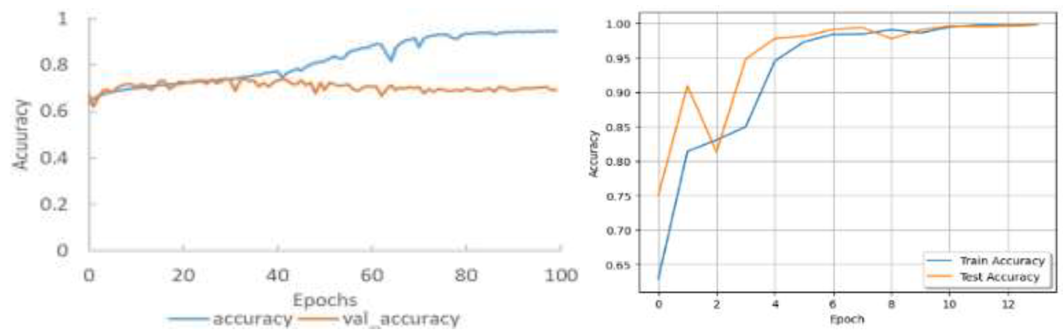
Figure 7. A Loss. The loss in the learning data was described as ‘loss’ and, that in the test data was described as ‘Val loss’.

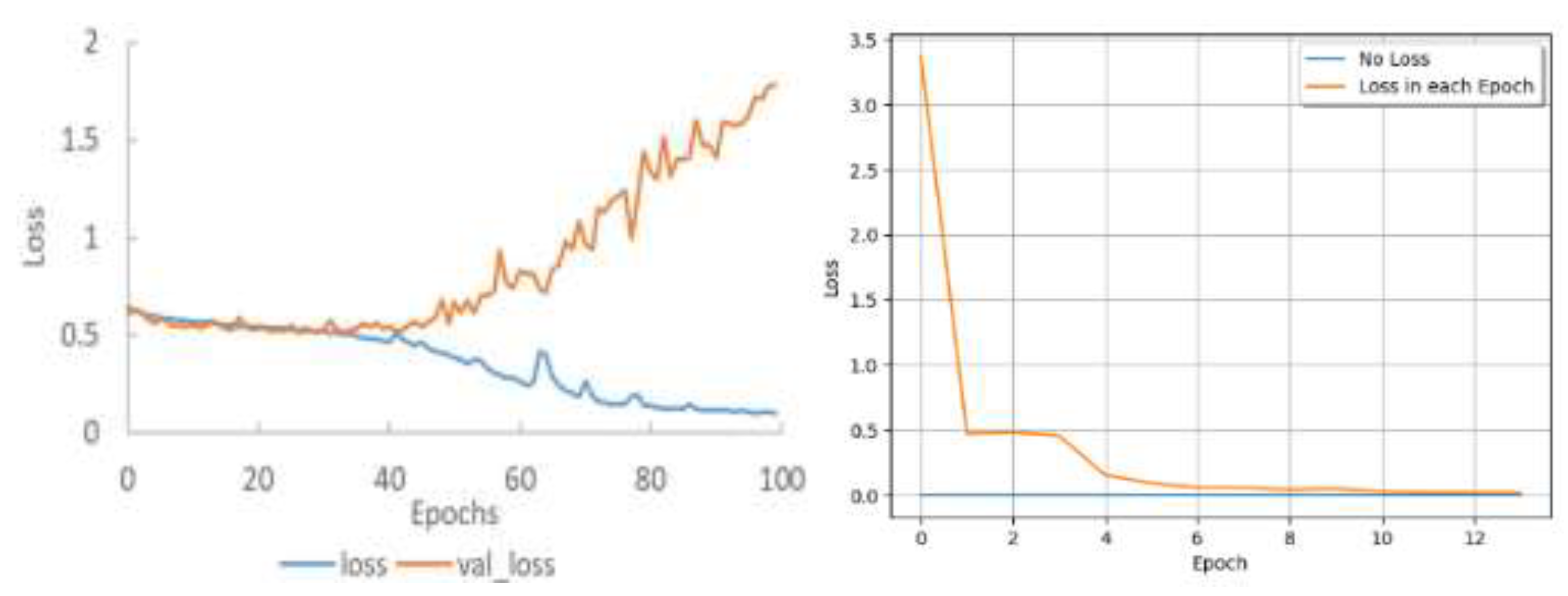
Table 2. Various results for trainING statistics.

Epoch	Train Loss		Train Accuracy
Epoch	Rao’s result	Our result	Rao’s result	Our result
1	1.0686	0.4713	55.53%	81.38%
2	1.0481	0.4813	52.83%	83.05%
3	0.9955	0.4554	55.18%	84.95%
4	0.9264	0.1532	59.97%	94.52%
5	0.9029	0.0916	61.36%	97.30%
6	0.9105	0.0580	60.84%	98.40%
7	0.8952	0.0573	61.01%	98.45%
8	0.8948	0.0409	61.18%	99.05%
9	0.8859	0.0484	61.88%	98.60%
10	0.8875	0.0263	62.05%	99.45%
11	0.8824	0.0188	62.75%	99.74%

Table 3. Performance analysis of THE trained models.

Epoch	Batch size	Accuracy (%)	AUC	Specificity
10 20 20 20 20 20	10 32 32 32 32 32	87.20% 76.20% 88.00% 89.90% 89.00% 86.82%	0.8244 0.6589 0.8286 0.8088 0.8417 0.6819	87.20% 76.20% 88.00% 89.90% 89.00% 86.82%

Disclaimer/Publisher’s Note: The statements, opinions and data contained in all publications are solely those of the individual author(s) and contributor(s) and not of MDPI and/or the editor(s). MDPI and/or the editor(s) disclaim responsibility for any injury to people or property resulting from any ideas, methods, instructions or products referred to in the content.

© 2024 by the authors. Licensee MDPI, Basel, Switzerland. This article is an open access article distributed under the terms and conditions of the Creative Commons Attribution (CC BY) license (http://creativecommons.org/licenses/by/4.0/).

Copyright: This open access article is published under a Creative Commons CC BY 4.0 license, which permit the free download, distribution, and reuse, provided that the author and preprint are cited in any reuse.