Submitted:
15 January 2025
Posted:
15 January 2025
You are already at the latest version
Abstract
Whale signals originating in the vicinity of a triplet of underwater hydrophones, 2 km distant from each other, and recorded at the three hydrophones, offer the opportunity to verify simple models of propagation applied in the immediate neighborhood of the triplet, by comparing arrival times and amplitudes between the three hydrophones. Examples of recordings of individual fin whales based on the characteristics of their vocalizations around 20 Hz, passing by hydrophone triplets are presented. Conclusions are drawn about waveform coherency and amplitudes of the signals recorded at the three hydrophones in the [10-50] Hz frequency band. A grid-search method of tracking the calls is presented based on time differences of arrivals between three hydrophones obtained with a combination of power detector time picking and cross-correlation. The spherical amplitude decay law of one over the distance is verified using amplitude ratios between two of the hydrophones, when the cetacean is in the immediate vicinity of the triplet, in a circle of radius 1.5 km sharing its center with the triplet. In turn, the measurement of the amplitude ratios between two hydrophones allows for an estimate of the depth of vocalization when the animal is within 250 m of horizontal distance of one of the hydrophones. Analysis of hundreds of calls leads to the possibility that more accurate coordinates and depth of the hydrophones are needed to unambiguously verify the laws of propagation, or that more elaborate non-isotropic models of propagation are needed.
Keywords:
1. Introduction
2. Data Acquisition and Processing Methods
2.1. Data Acquisition
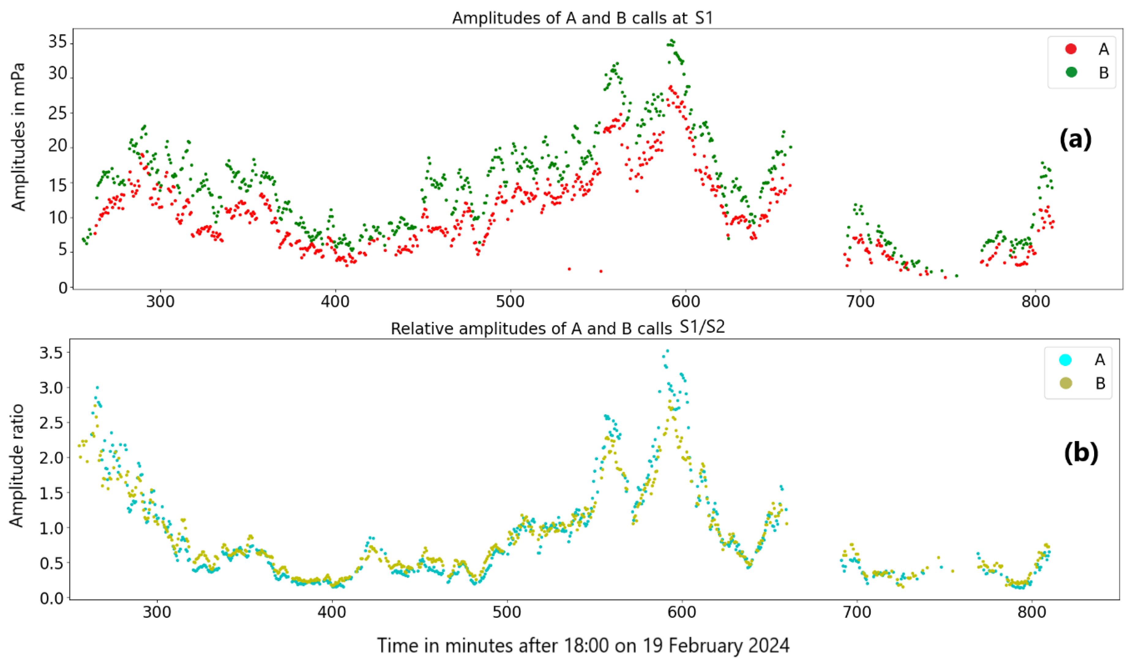
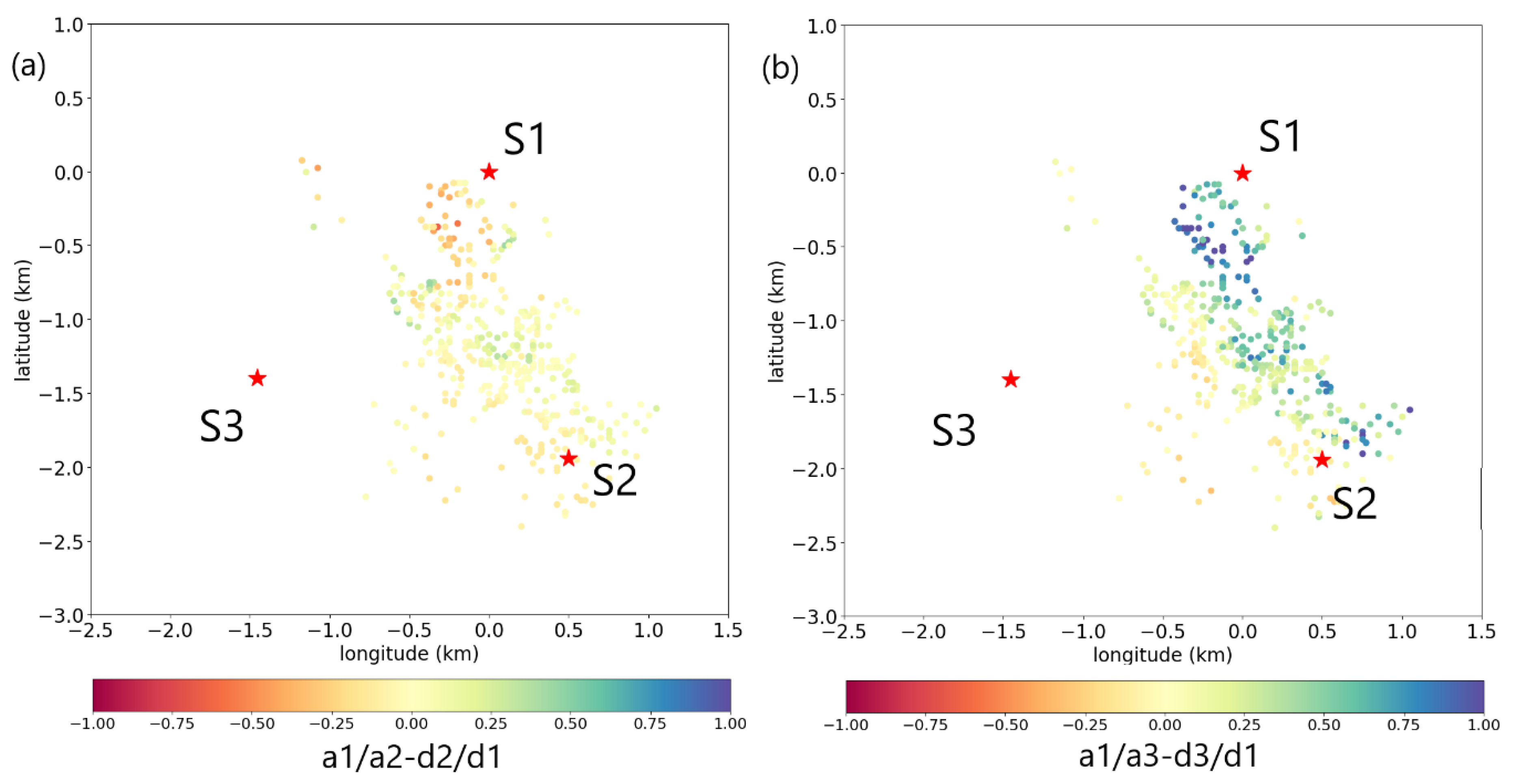
- The amplitude of the signal is increasing on all three waveforms starting from about one hour after time zero. This can easily be explained if the source is progressively getting closer to all three sensors until the end of the two-hour sequence.
- The amplitudes at S1 and S3 are slightly higher than at S2.
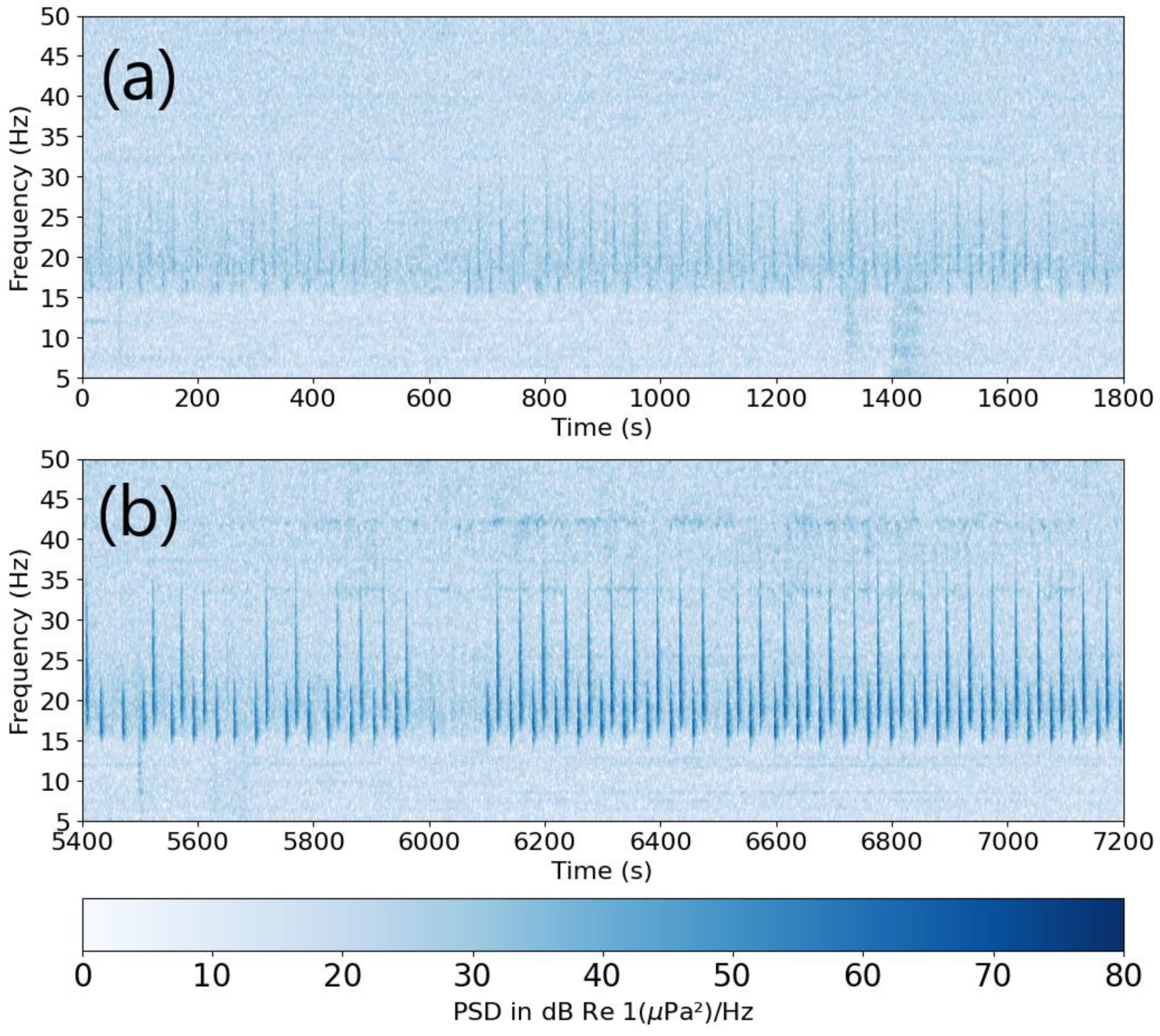
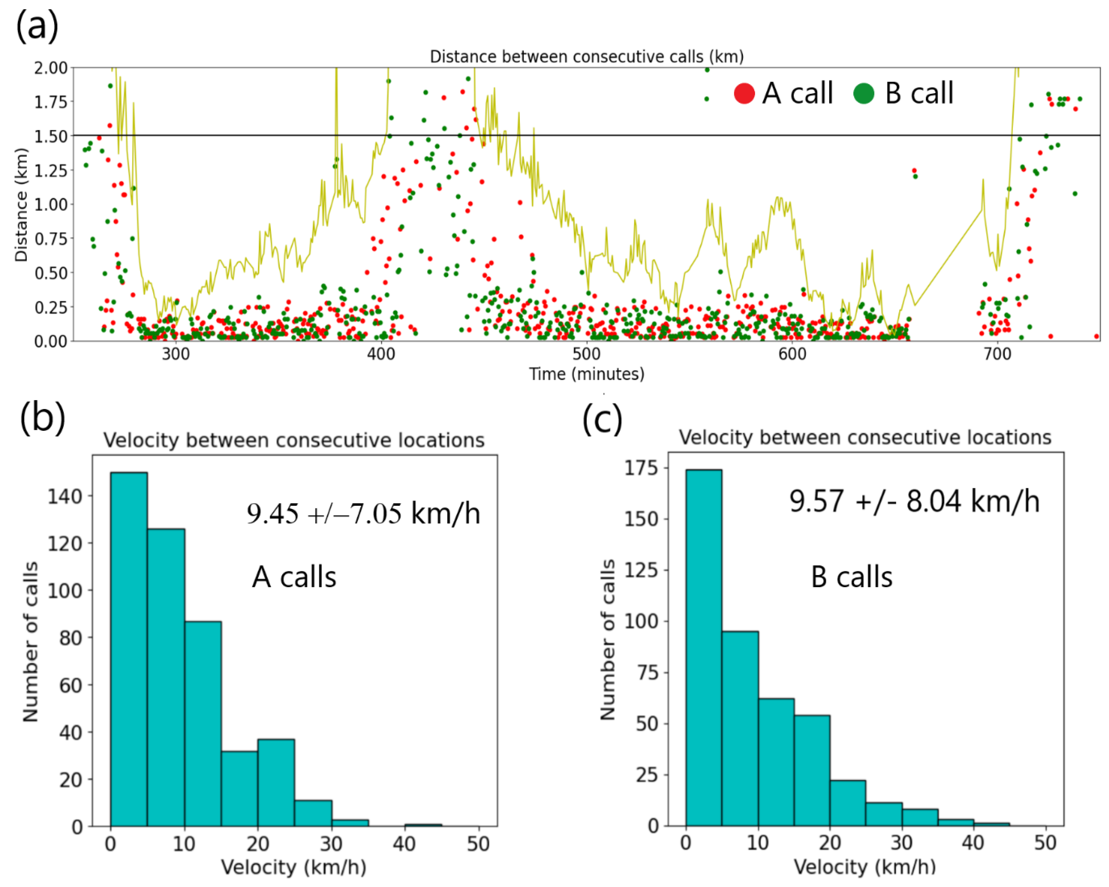
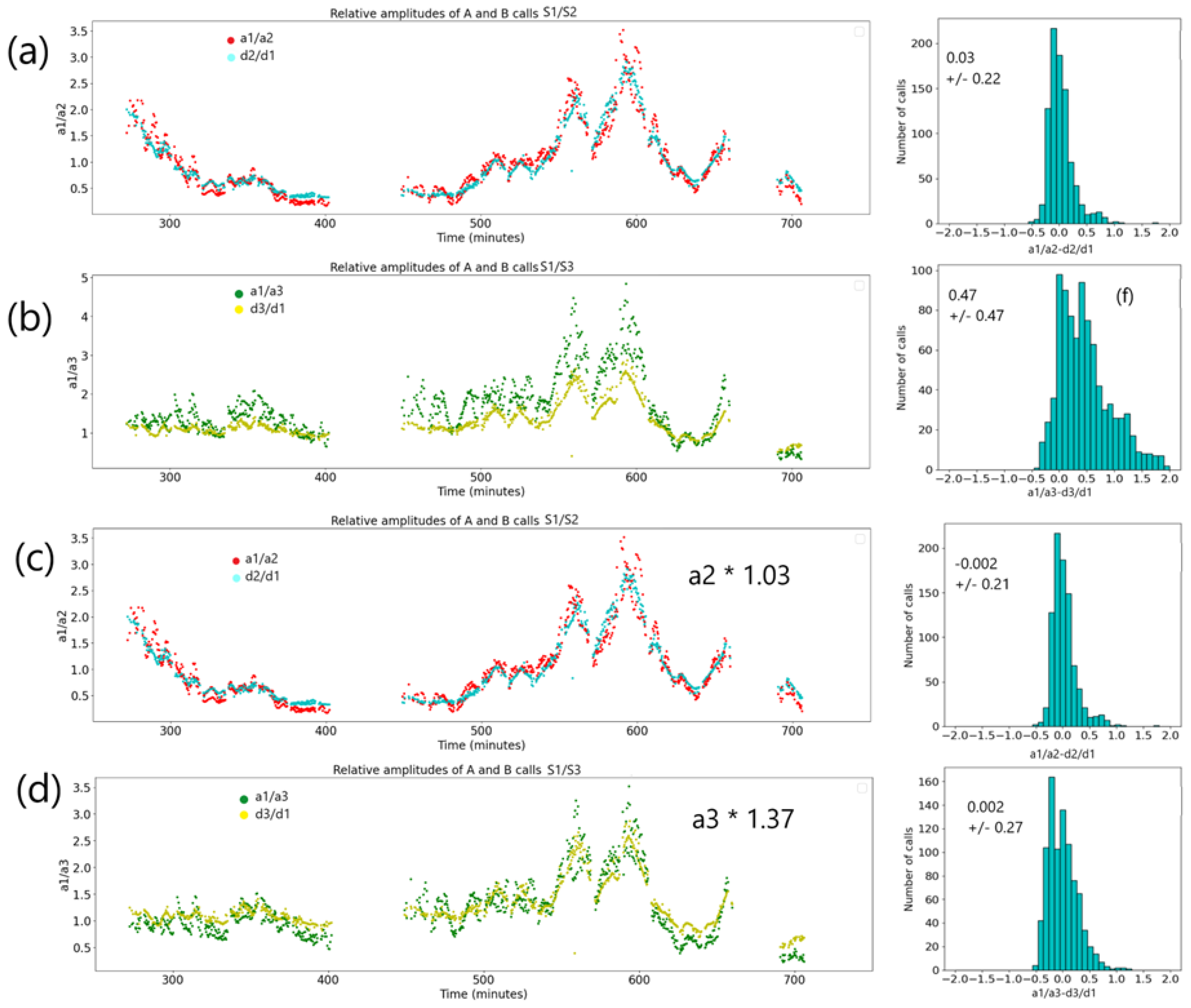
- Two types of calls are clearly visible on the spectrogram. One type has a broader bandwidth [17-40] Hz and higher center frequency than the other one [15-25] Hz. The nomenclature type A for the lower frequency type and type B for the higher frequency have previously been used in the literature[19]. The two types are separated by about 25 s and generally alternate, but not always. An exception can be seen in Figure 2 in an interval of about 100 s after 5600 s with three consecutive type B in that interval, and again twice at about 5800 s. Each call is picked individually, and the measurement of amplitudes shows a bimodal distribution corresponding to these two types.
- If the hypothesis that the interruptions in the calls are at the time of surfacing, and the calls originate with a single individual, the first call when the animal dives is generally the lower, narrower band, frequency pulse (type A), and the last call is the higher, broader band, frequency call (type B)
2.2. Waveform Signal Processing
| Algorithm 1 | DTOA and amplitudes extraction | |
|
Input: Three waveform segments from S1, S2, S3. Output: Three arrays of time differences d12, d23, d31 and three arrays of amplitudes a1, a2, a3. All six arrays are of dimension Ndet, the number of groups of three detections (one each at S1, S2, S3) made. | ||
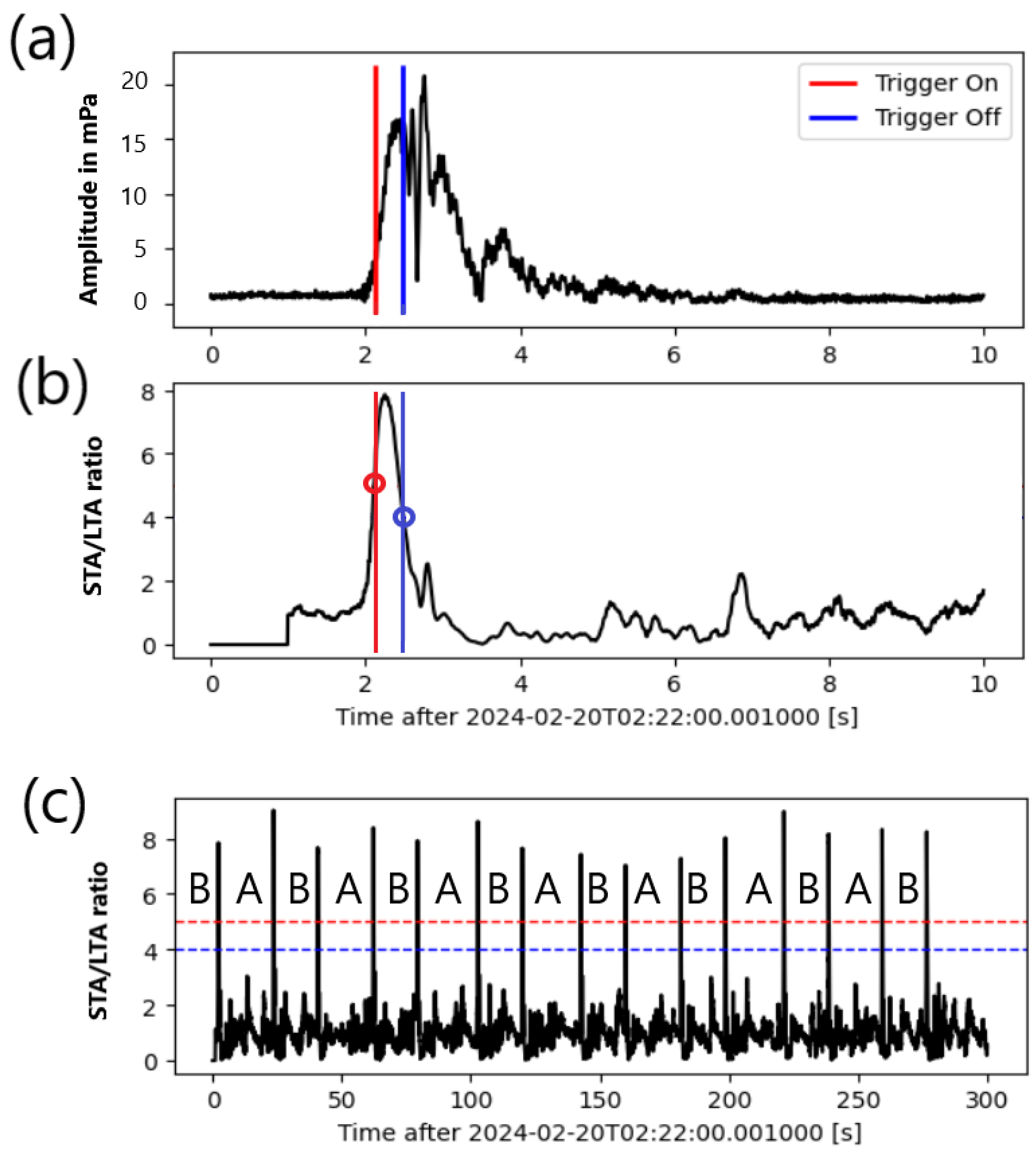
| Step 1 | Apply STA/LTA algorithm on all three waveforms. Get N1, N2, N3 detections respectively on S1, S2, S3. | |
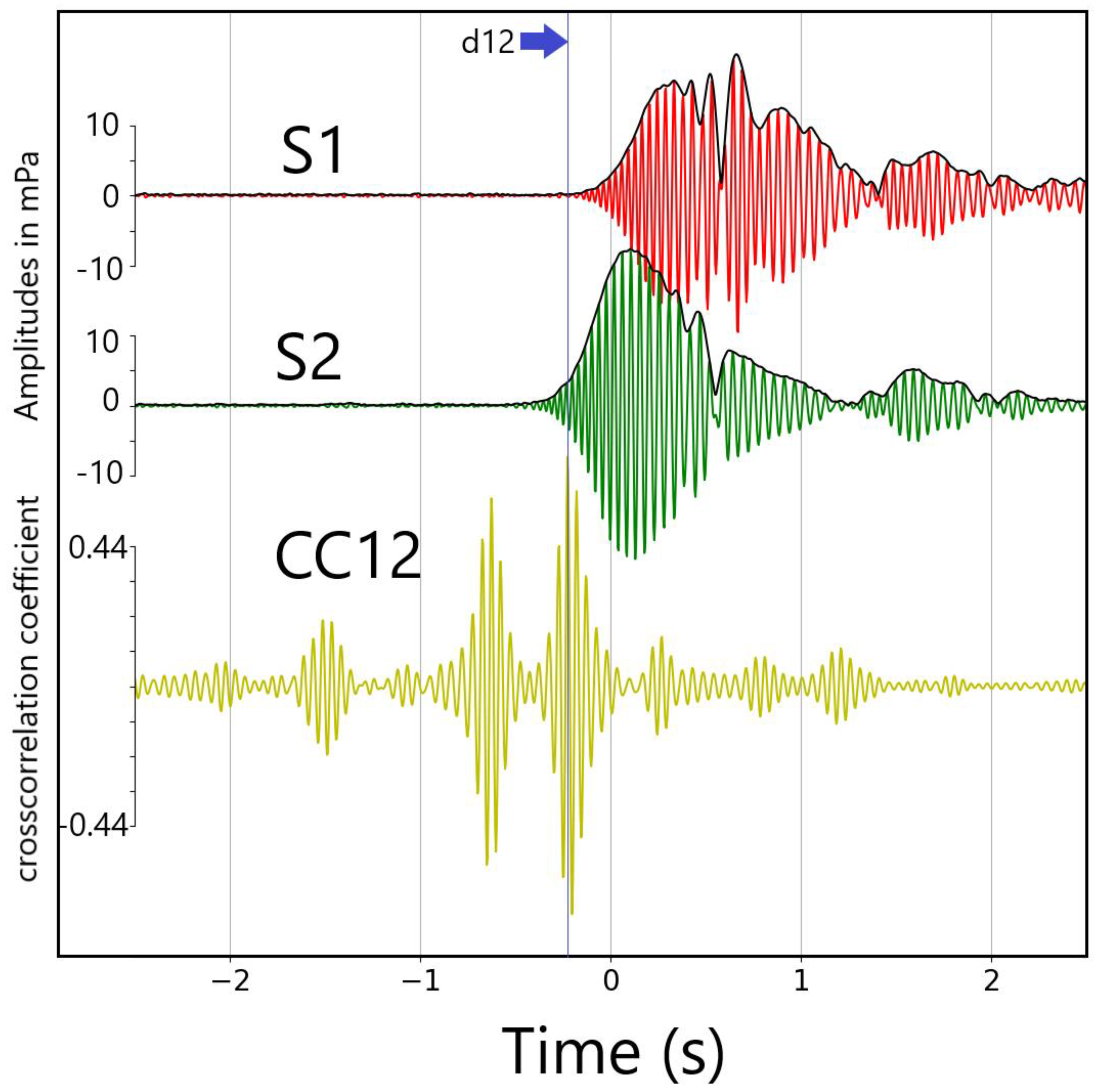
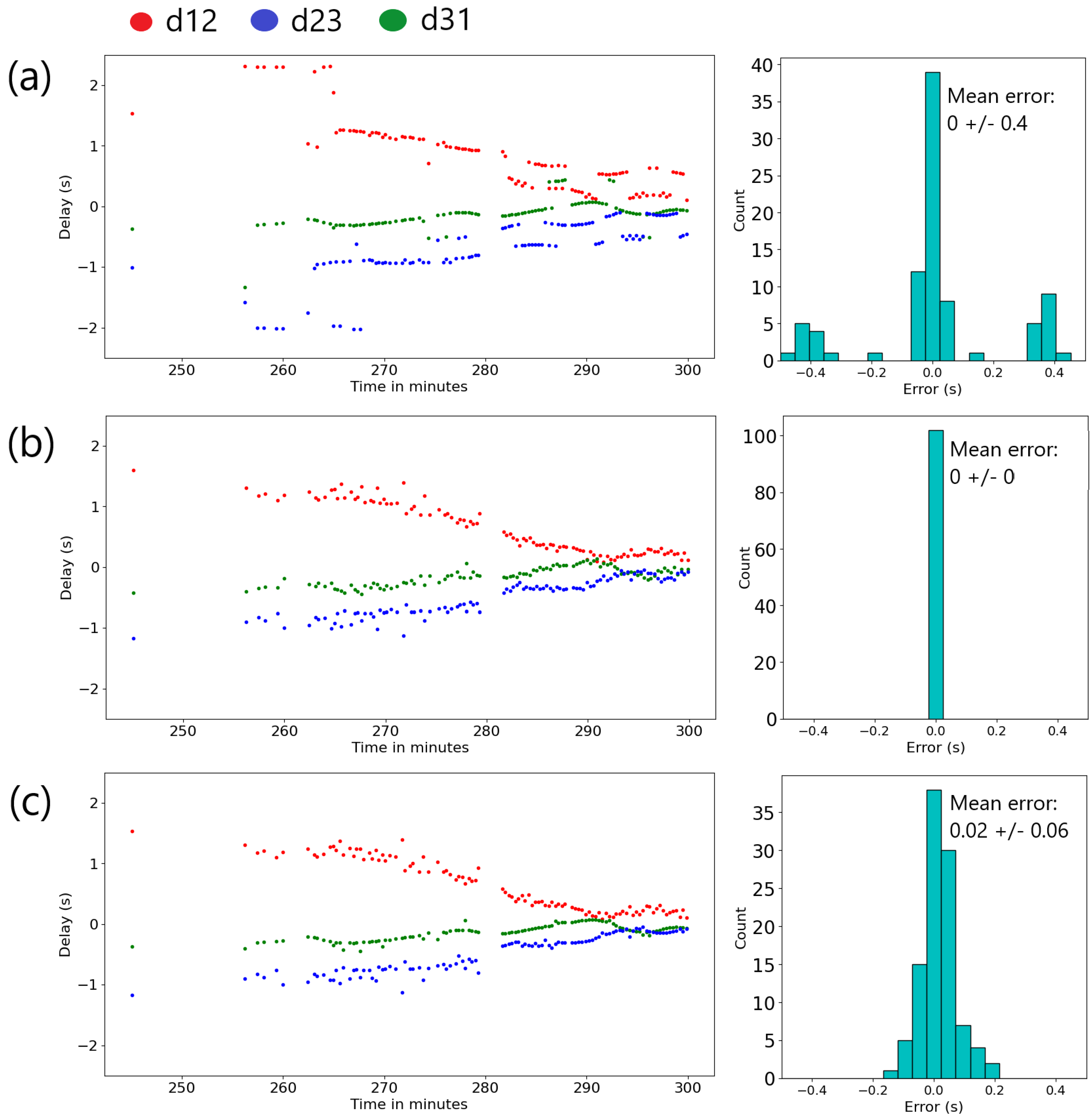
| Step 2 | For each detection at S1: Cross-correlate waveform 10 s segments (start time 2.5 s before t1[i]) within each group, Extract cd12[i], cd23[i], cd31[i], time difference estimates from the maximum of the cross-correlation. These are illustrated in Figure 5a. | |
| Step 3 | For each detection at S1: If detections exist for S2 and S3, compatible with a single call detected at all three hydrophones, group them with the S1 detection. This results in Ndet groups of detections where Ndet < = N1. | |
| Step 4 | For each group, calculate Ndet DTOA as d12[i] = t2[i]-t1[i], d23[i] = t3[i]-t2[i], d31[i] = t1[i]-t3[i], time difference estimates from the STA/LTA pick times. These are illustrated in Figure 5b. | |
| Step 5 | Adjust DTOA as d12[i] = cd12[i] if abs(cd12[i] – d12[i]) < 0.1 s., and similarly for 23 and 31. These are illustrated in Figure 5c. | |
| Step 6 | Extract amplitudes a1, a2, a3, as the maxima of the envelopes on the 10 s segments. These are illustrated in Figure 6. | |
2.3. Location Method by Grid Search
| Algorithm 2 | Grid search for optimal location | |
|
Input: Three DTOA scalar arrays d12, d23, d31 of length Ndet. Output: Optimal locations of all Ndet calls for a given constant depth. | ||
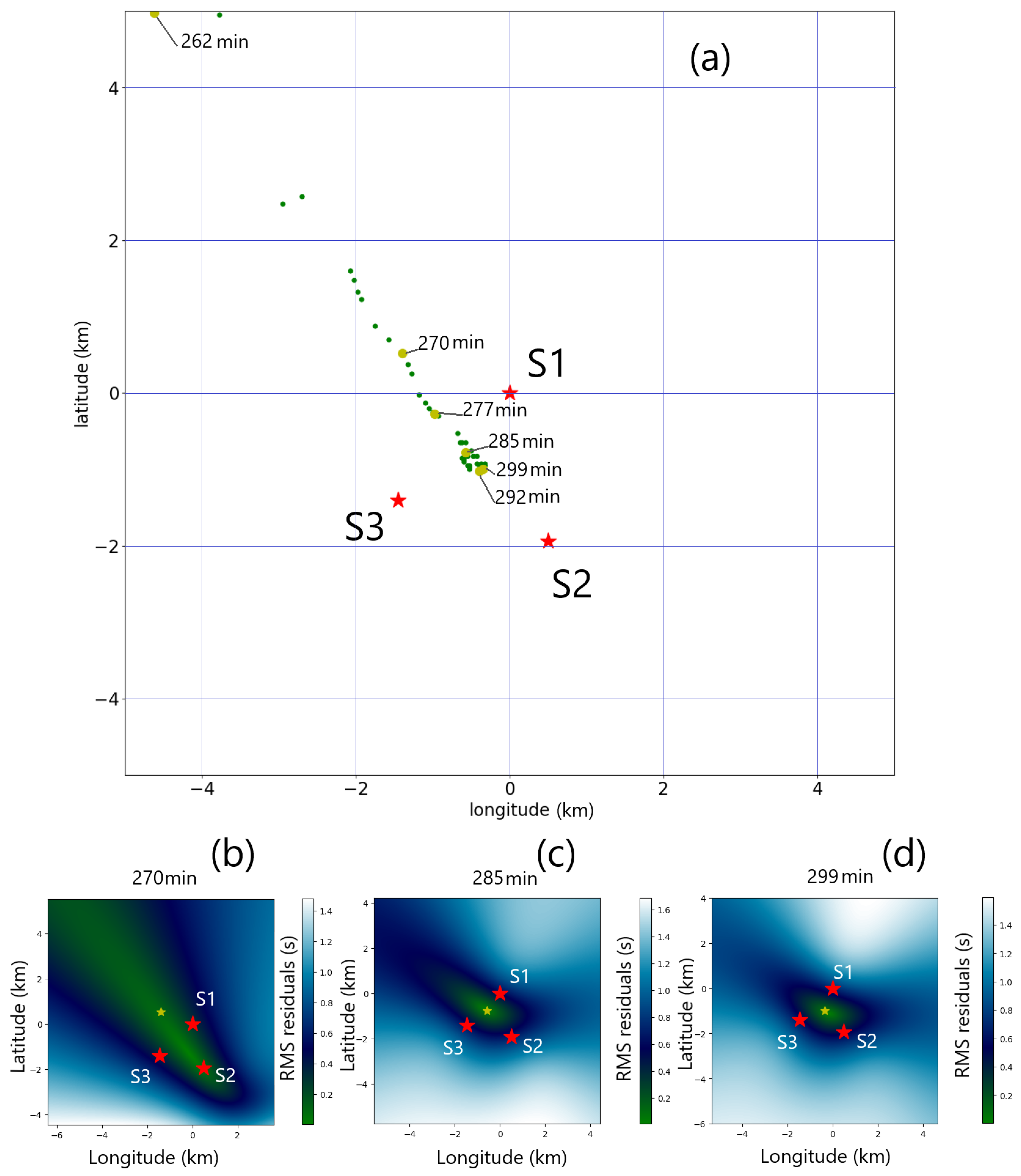
| Step 1 | For the initial point d12[1], assume whale depth of zero, water velocity v = 1480 m/s, and straight-line propagation. For each point of a horizontal 400x400 grid, with 25 m spacing (10 km by 10 km), compute the RMS of the difference between the observed and estimated DTOA: , where td12 is the theoretical travel time difference between propagation to S2 and propagation to S1: , where denotes the distance between points A and B. |
|
| Step 2 | X[1] is the grid point [p, q]opt with the lowest value of res[p, q] over all p and q grid points. | |
| Step 3 | For later groups of detections, search a 40x40 grid around X[i-1], with the same 25 m spacing (1km by 1 km). The reason for a smaller grid is that the whale cannot move further than 0.5 km within the time between consecutive calls. | |
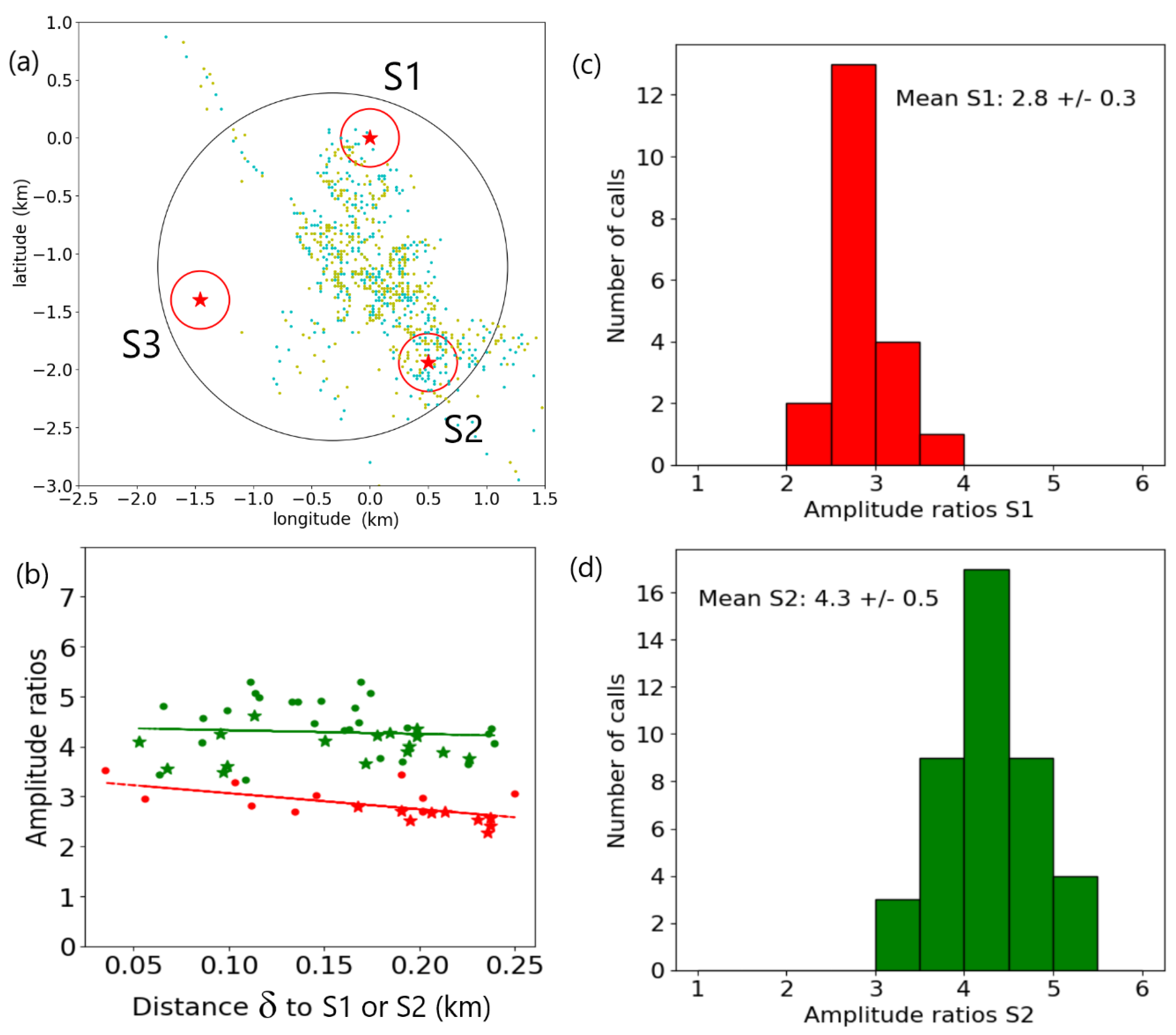
2.4. Amplitude Ratios When the Whale Is Directly Above a Hydrophone
3. Results
3.1. Location by Grid Search for the Initial Two-Hour Onset of Observations
3.2. Location and Amplitude Results on the Whole Seventeen Hours of Observations
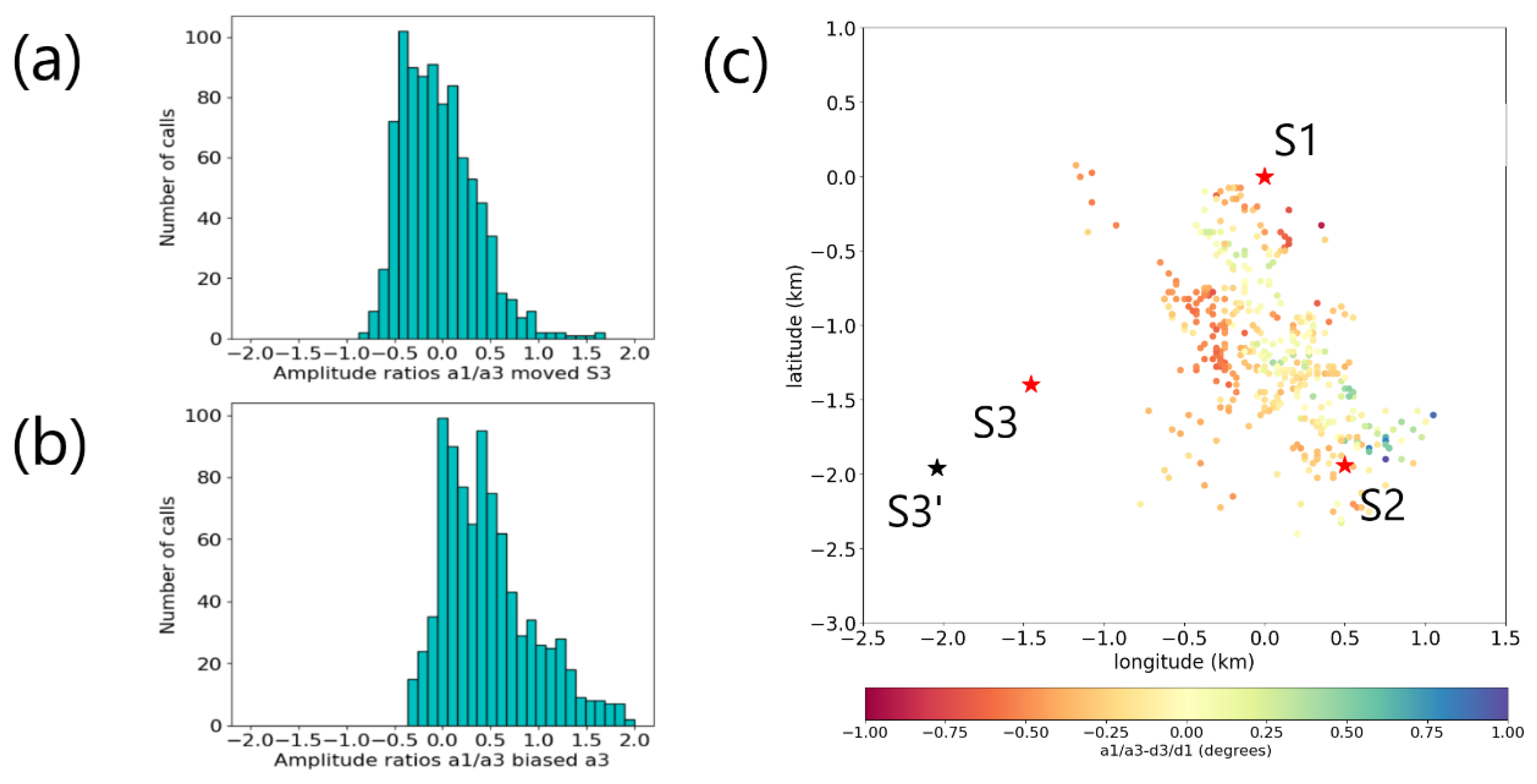
3.2. Taking Advantage of Dense Coverage Close to S1 and S2 to Estimate Depths
4. Discussion
5. Conclusions
Author Contributions
Funding
Data Availability Statement
Conflicts of Interest
References
- CTBTO. Available online: www.ctbto.org (accessed on 12 November 2024).
- IMS map. Available online: https://www.ctbto.org/sites/default/files/2024-10/IMS_Map_FRONT_BACK_AUGUST_2021_web2.pdf (accessed on 12 November 2024).
- International Whaling Commission. Available online: https://iwc.int/about-whales (accessed on 7 July 2024).
- Munk, W.H. Sound channel in an exponentially stratified ocean with applications to SOFAR. J. Acoust. Soc. Am. 1974, 55, 220–226. [Google Scholar] [CrossRef]
- Thode, A. Tracking sperm whale (Physeter macrocephalus) dive profiles using a towed passive acoustic array. J. Acoust. Soc. Am. 2004, 116, 245–253. [Google Scholar] [CrossRef] [PubMed]
- Thode, A.M.; Kim, K.H.; Blackwell, S.B.; Greene, C.R.; Nations, C.S.; McDonald, T.L.; Macrander, A.M. Automated detection and localization of bowhead whale sounds in the presence of seismic airgun surveys. J. Acoust. Soc. Am. 2012, 131, 3726–3747. [Google Scholar] [CrossRef]
- Miksis-Olds, J.L.; Harris, D.V.; Heaney, K.D. Comparison of estimated 20-Hz pulse fin whale source levels from the tropical Pacific and Eastern North Atlantic Oceans to other recorded populations. J. Acoust. Soc. Am. 2019, 146, 2373–2384. [Google Scholar] [CrossRef] [PubMed]
- Harris, D.V.; Miksis-Olds, J.L.; Vernon, J.A.; Thomas, L. Fin whale density and distribution estimation using acoustic bearings derived from sparse arrays. J. Acoust. Soc. Am. 2018, 143, 2980–2993. [Google Scholar] [CrossRef]
- Balcazar, N.E.; Tripovich, J.S.; Klinck, H.; Nieukirk, S.L.; Mellinger, D.K.; Dziak, R.P.; Rogers, T.L. Calls reveal population structure of blue whales across the southeast Indian Ocean and the southwest Pacific Ocean. J. Mammal. 2015, 96, 1184–1193. [Google Scholar] [CrossRef] [PubMed]
- Gavrilov, A.N.; McCauley, R.D.; Salgado-Kent, C.; Tripovich, J.; Burton, C. Vocal characteristics of pygmy blue whales and their change over time. J. Acoust. Soc. Am. 2011, 130, 3651–3660. [Google Scholar] [CrossRef] [PubMed]
- Gavrilov, A.N.; McCauley, R.D. Acoustic detection and long-term monitoring of pygmy blue whales over the continental slope in southwest Australia. J. Acoust. Soc. Am. 2013, 134, 2505–2513. [Google Scholar] [CrossRef]
- Le Bras, R.J.; Kuzma, H.; Sucic, V.; Bokelmann, G. Observations and Bayesian location methodology of transient acoustic signals (likely blue whales) in the Indian Ocean, using a hydrophone triplet. J. Acoust. Soc. Am. 2016, 139, 2656–2667. [Google Scholar] [CrossRef] [PubMed]
- Le Bras, R.; Nielsen, P. Range estimates of whale signals recorded by triplets of hydrophones, AGU Fall Meeting. 2017. [Google Scholar] [CrossRef]
- Sirovic, A.; Hildebrand, J.A.; Wiggins, S. Blue and fin whale call source levels and propagation range in the Southern Ocean. J. Acoust. Soc. Am. 2007, 122, 1208–1215. [Google Scholar] [CrossRef]
- Kuna, V.M.; Nábělek, J.L. Seismic crustal imaging using fin whale songs. Science 2021, 371, 731–735. [Google Scholar] [CrossRef] [PubMed]
- Stimpert, A.K.; DeRuiter, S.L.; Falcone, E.A.; et al. Sound production and associated behavior of tagged fin whales (Balaenoptera physalus) in the Southern California Bight. Anim Biotelemetry 2015, 3, 23. [Google Scholar] [CrossRef]
- Pereira, A.; Harris, D.; Tyack, P.; Matias, L. On the use of the Lloyd's Mirror effect to infer the depth of vocalizing fin whales. J. Acoust. Soc. Am. 2020, 148, 3086–3101. [Google Scholar] [CrossRef] [PubMed]
- Lloyd, Humphrey (1831). "On a New Case of Interference of the Rays of Light". The Transactions of the Royal Irish Academy. 17. Royal Irish Academy: 171–177. ISSN 0790-8113. JSTOR 30078788. Retrieved 2021-05-29.
- Zhu, J.; Wen, L. Hydroacoustic study of fin whales around the Southern Wake Island: Type, vocal behavior, and temporal evolution from 2010 to 2022. J. Acoust. Soc. Am. 2024, 155, 3037–3050. [Google Scholar] [CrossRef] [PubMed]
- Various Institutions. (1965). International Miscellaneous Stations [Data set]. International Federation of Digital Seismograph Networks. [CrossRef]
- Lawrence, M., G. Haralabus, M. Zampolli, D. Metz, (2024). Comprehensive Nuclear-Test-Ban Treaty Organization, Vienna, (2024). The Comprehensive Nuclear-Test-Ban Treaty Hydroacoustic Network, in Kalinowski, M.B., Haralabus, G., Labak, P., Mialle, P., Sarid, E., Zampolli, M. (eds); Published by the Provisional Technical Secretariat of the Preparatory Commission for the Comprehensive Nuclear-Test-Ban Treaty Organization, Austria. Available online: https://www.ctbto.org/sites/default/files/2024-07/20240618-CTBTO%2025th%20Anniversary%20booklet%20Final%20HRes.pdf (accessed on 8 August 2024).
- Watkins, W.A.; Tyack, P.; Moore, K.E.; Bird, J.E. The 20-Hz signals of finback whales (Balaenoptera physalus). J. Acoust. Soc. Am. 1987, 82, 1901–1912. [Google Scholar] [CrossRef]
- Trnkoczy, A. Understanding and parameter setting of STA/LTA trigger algorithm. In New Manual of Seismological Observatory Practice 2 (NMSOP-2); Bormann, P., Ed.; Deutsches GeoForschungsZentrum GFZ: Potsdam, 2012; pp. 1–20. [Google Scholar] [CrossRef]
- Allen, R.V. Automatic earthquake recognition and timing from single traces. Bull. seism. Soc. Am. 1978, 68, 1521–1532. [Google Scholar] [CrossRef]
- Le Bras, R.J.; Mialle, P.; Kushida, N.; Bittner, P.; Nielsen, P. Developments in Hydroacoustic Processing for Nuclear Test Explosion Monitoring. In Kalinowski, M.B., Haralabus, G., Labak, P., Mialle, P., Sarid, E., Zampolli, M. (eds); Published by the Provisional Technical Secretariat of the Preparatory Commission for the Comprehensive Nuclear-Test-Ban Treaty Organization, Austria. 2024. 2024. Available online: https://www.ctbto.org/sites/default/files/2024-07/20240618-CTBTO%2025th%20Anniversary%20booklet%20Final%20HRes.pdf (accessed on 8 August 2024).
- Cansi, Y.; Le Pichon, A. Infrasound Event Detection Using the Progressive Multi-Channel Correlation Algorithm. In Handbook of Signal Processing in Acoustics; Springer: New York, NY, USA, 2009; pp. 1425–1435. [Google Scholar]
- Yi, B.Y.; Lee, G.H.; Kim, H.J.; Jou, H.T.; Yoo, D.G.; Ryu, B.J.; Lee, K. Comparison of wavelet estimation methods. Geosci. J. 2013, 17. [Google Scholar] [CrossRef]
- Braving storms. Constructing hydroacoustic station HA11 Wake Island. Available online: https://www.ctbto.org/news-and-events/news/braving-storms-constructing-hydroacoustic-station-ha11-wake-island (accessed on 22 July 2024).
- VDEC. Available online: https://www.ctbto.org/resources/for-researchers-experts/vdec (accessed on 10 July 2024).
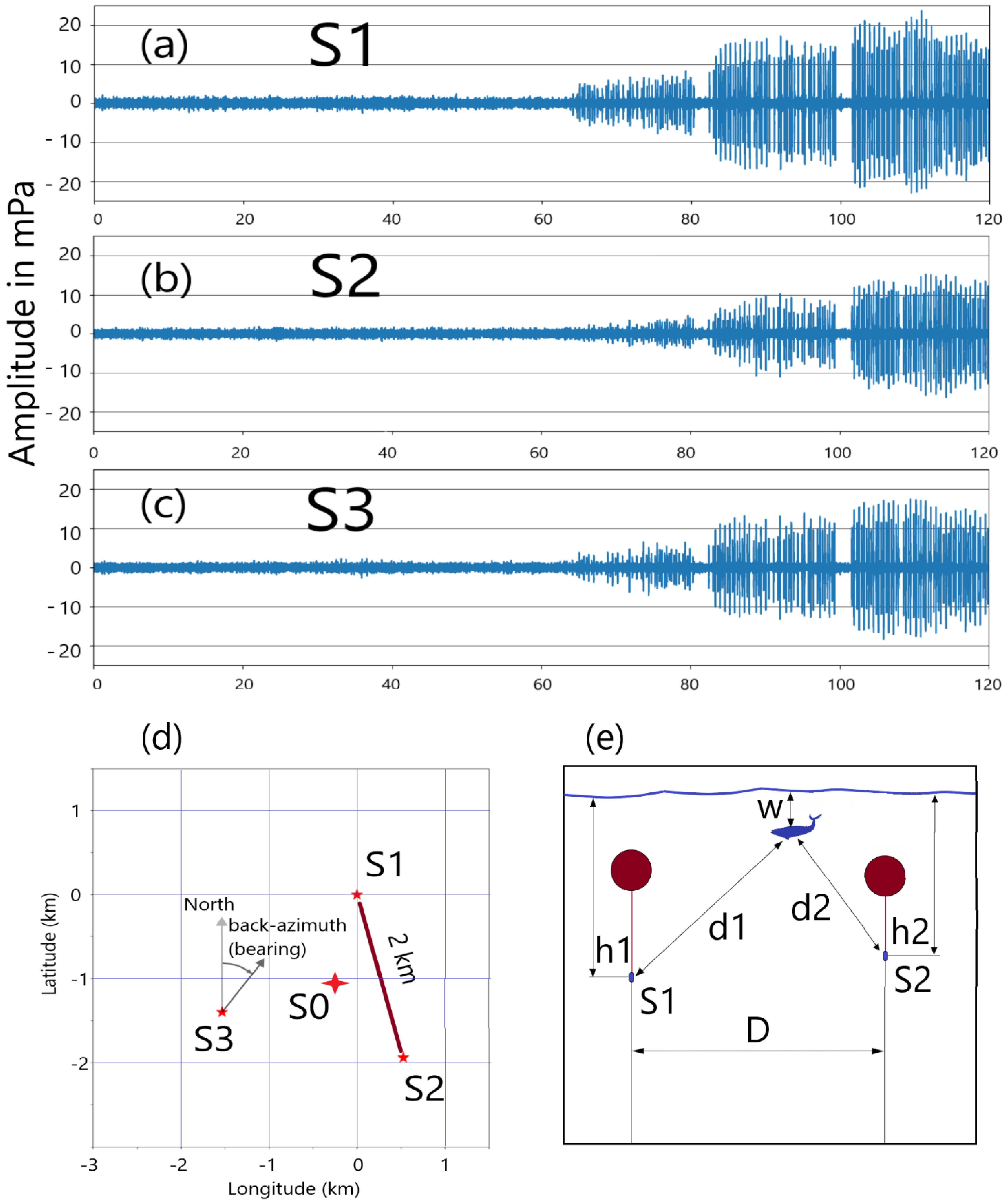

| Hydrophone | Identifier | Latitude Longitude* (decimal degree) |
Latitude Longitude (km from S1) |
Depth (m) |
|
|---|---|---|---|---|---|
| H11S1 | S1 | 18.50827 166.700272 |
0.000 0.000 |
h1 | 739** 750* |
| H11S2 | S2 | 18.49082 166.705002 |
-1.939 0.498 |
h2 | 739** 742* |
| H11S3 | S3 | 18.49568 166.686462 |
-1.399 -1.455 |
h3 | 739** 724* |
| Hydrophone | Amplitude ratios | h1 = 739 m h2 = 739 m |
h1 = 750 m h2 = 742 m |
|---|---|---|---|
| S1 | r1 = 2.8 | w1 = 28 m | w1 = 51 m |
| r1 = 3.4 | w1 = 167 m | w1 = 191 m | |
| S2 | r2 = 4.3 | w2 = 295 m | w2 = 284 m |
| r2 = 4.4 | w2 = 305 m | w2 = 295 m |
Disclaimer/Publisher’s Note: The statements, opinions and data contained in all publications are solely those of the individual author(s) and contributor(s) and not of MDPI and/or the editor(s). MDPI and/or the editor(s) disclaim responsibility for any injury to people or property resulting from any ideas, methods, instructions or products referred to in the content. |
© 2025 by the authors. Licensee MDPI, Basel, Switzerland. This article is an open access article distributed under the terms and conditions of the Creative Commons Attribution (CC BY) license (http://creativecommons.org/licenses/by/4.0/).


