
Submitted:
15 October 2024
Posted:
15 October 2024
You are already at the latest version
Abstract
The distribution of impervious surface is one of the important assessment indicators for evaluating the quality of urban ecological environment. Taking Xuzhou city as an example, we study the influence of the spatial distribution of impervious surfaces on urban surface temperature, using Landsat 8 remote sensing imagery and nighttime lighting data to extract the impervious surface information from 2013 to 2022 and carry out surface temperature inversion. The study area was divided into built-up and non-built-up areas using nighttime lighting data and the relevant indices were used to establish interest zones and finally the extraction of impervious surfaces was completed using supervised classification methods. The experimental results show that the kappa coefficient is not less than 0.8562, which makes the result more reliable. By extracting the impervious surface of Xuzhou City, it was found that the impervious surface of Xuzhou City continued to increase from 2013 to 2022, in which the growth rate was faster in 2014-2016 and 2019-2021, and slowed down in 2017-2018 and 2021-2022. The expansion of impervious surface was found to be one of the reasons for the increase of urban surface temperature through stacked analysis and linear regression analysis.
Keywords:
impervious surface
; land surface temperature
; supervision and classification
; spatio-temporal variation
1. Introduction
Cyclical monitoring of urbanization processes, ecological changes, and land-use patterns is conducive to the sustainable development of urban agglomerations. Impervious Surface Area (ISA) is one of the important indicators for evaluating the degree of urbanization, which mainly includes surfaces with small permeability such as roofs, parking lots, and roads [1]. The degree of urbanization and the percentage of impervious surfaces are closely related, and impervious surfaces continue to replace natural surfaces such as vegetation, farmland, and rivers in the process of large-scale urbanization, which can easily lead to a series of environmental problems [2,3,4]. With urban development, the urban green area shrinks and the impervious surface expands, leading to a gradual increase in urban surface temperature. This can easily cause the urban heat island effect, so it is important to study the effect of impervious surface on surface temperature to predict and control the urban surface temperature [5].
The main methods of impervious surface extraction are the exponential method, spectral mixture analysis, and regression method. The exponential modeling approach is used to extract information about features based on differences in reflections of various features at different ranges by constructing a mathematical model. Some of the widely used exponential models are P-index, Impervious surface Area Index (ISA), Normalized Impervious Surface Index(NDISI), Modified Normalized Difference Impervious Surface Index (MNDISI), and triple-exponential methods, among others [6,7,8,9]. The ISA index can effectively differentiate between vegetated and impervious surfaces, but ignores the effects of soils and water bodies, and has a narrower scope of application, applying only to areas where the cover type is predominantly impervious and vegetated. The NDISI index can more accurately distinguish between different land cover types in urban areas and can better minimize the influence of soil on impervious surface extraction, but the classification accuracy is low [10,11]. The MNDISI index is based on the NDISI index combined with high-resolution nighttime light data to improve the extraction accuracy, but the nighttime light data are difficult to obtain, and the water body needs to be masked before use, which is a complicated process with many processing steps, and the application is limited [12]; Mu Yachao et al. proposed a new Enhanced Impermeable Surface Index (ENDISI), which can effectively eliminate the interference of sandy bare ground in arid areas [13]. The construction of the P-index integrates the impervious surface index, the Index-based Build-up Index (IBI), and the inverted impervious surface information, which is extracted with high accuracy, but is difficult to compute and poorly operationalized [14]. Biophysical Composition Index (BCI), Comprehensive Cumulative Index (CBI), and IBI Construction Index belong to the triple index method, and the problem of confusing information on impervious surfaces using this algorithm still exists, making it difficult to ensure accuracy [15,16]. The index method is simple and easy to compute, and can quickly and accurately extract impervious surfaces, but the index construction process is complicated and has low generalizability, in addition, due to the limitation of spatial resolution, there are mixed pixels in the image, which can easily lead to misclassification of features.
Spectral mixing analysis utilizes a chunking method that allows for the determination of the proportions of the spectral components of different features in the same image element. Ridd et al. proposed a new surface model called the vegetation-impervious-soil (V-I-S) model [17]. The model views the surface as an assemblage of vegetation, impervious surfaces, and soils, and attributes the spectral response of different surface types to the relative proportions of these three components. Based on this idea, Roberts et al. developed and tested the Multiple Endmember Spectral Mixture Analysis (MESMA) [18]. Wu et al. improved the linear spectral decomposition method by dividing the surface into four categories: vegetation, soil, high albedo features, and low albedo features, and summing the high albedo and low albedo features to obtain the urban distribution in the Columbus area [19]. Spectral mixing analysis solves the problem of mixing pixels on low and medium spatial resolution images to a certain extent, but there are still limitations in this method, the complexity of feature types in the city, the spectral heterogeneity of impervious surfaces is strong, and the selection of endpoints is subjective, especially for the selection of endpoints in large areas is more difficult. At the same time, there are errors in the decomposition results of different features and coverage in the hybrid image element, which can easily lead to the underestimation of areas with high coverage of impervious surfaces easily using the SMA method, and the overestimation of areas with low coverage [20].
In summary, it can be seen that the key to ensuring the accuracy of impervious surface extraction is the ability to distinguish the impervious surface from bare soil. Most of the impervious surfaces are distributed in built-up areas, and the use of the impervious surface index to establish an impervious surface area of interest at the impervious surface aggregation can effectively reduce the probability of bare soil being misclassified as impervious surfaces, thus effectively ensuring the accuracy of the extraction of impervious surfaces in the area. The brightness information of nighttime lighting data can directly reflect the location of built-up areas within the study area, therefore, the comprehensive application of nighttime lighting data and remote sensing image data can effectively improve the accuracy of impervious surface extraction [21]. Elvidge et al. established a global impervious surface model based on DMSP-OLS and TM data [22]. Cheng Xi et al. integrated spatial and spectral information from nighttime lights and Landsat TM images to realize the identification of impervious surfaces [23]. Tang Pengfei et al. constructed a feature set by spectral and texture features and then used nighttime lighting information and spectral information to select positive and negative samples of impervious surfaces to complete the extraction of impervious surfaces [24], which effectively reduces the influence of bare soil on the extraction of impervious surfaces.
For this purpose, the luminance information of DMSP-OLS-like data [25] is used to obtain the vector map of built-up areas using the spatio-temporal normalized thresholding method based on pseudo-invariant features. Classification samples of water bodies, vegetation, and bare soil were established in the complete image using the corresponding indices, and impervious surface classification samples were established in the built-up area using the enhanced impervious surface index, and the extraction of impervious surfaces was accomplished using the maximum likelihood classification method. Surface temperature inversion was performed using Landsat8 OLI/TIRS C2L2 imagery and surface temperatures were categorized into high-temperature, sub-high-temperature, medium-temperature, sub-low-temperature, and low-temperature zones based on the mean-covariance method. The following analyses were performed to investigate the effect of impervious surfaces on surface temperature:(1) Overlay analysis of the impervious surface extraction results from 2013-2022 and the results after surface temperature grading in Xuzhou City showed that more than 50% of the impervious surface area is a high-temperature zone or a sub-high-temperature zone; (2) According to the density of impervious surfaces, Xuzhou City is divided into three parts: impervious surface aggregation area, permeable surface area and other impervious surface area, and the average temperatures of the above three areas are calculated respectively, and it is found that the average temperature of the impervious surface aggregation area is the highest, followed by the other impervious surface area, and the average temperature of the permeable surface area is the lowest. (3) A certain number of samples were selected in and around the built-up area, and the impervious surface density and average temperature of the selected sample areas were calculated and analyzed by linear regression. The results show that surface temperature and impervious surface density are directly proportional. In conclusion, the increase in impervious surface is one of the reasons for the increase in surface temperature, so the monitoring of impervious surface is of great significance for the management of the urban environment.
2. Impervious Surface Extraction Method
Determine the threshold value of built-up area using the spatio-temporal normalized threshold method based on pseudo-invariant features in night-time light images to realize the extraction of built-up area, use the corresponding index to establish the classification samples of water bodies, vegetation, and bare soil, respectively, and use the enhanced impervious surface index to establish the impervious surface samples in the built-up area, and finally use the maximum likelihood classification method to complete the extraction of impervious surfaces. Using the above method to accomplish impervious surface extraction has the following advantages:(1) The selected built-up area extraction method can quickly determine the thresholds for subsequent years using linear regression analysis after determining the thresholds for the selected base year, which reduces the influence of human subjective factors and makes the built-up area extraction results more stable and reliable;(2) Creating classification samples using impervious surface, vegetation, water body, and bare soil indices eliminates the need to manually select training samples and allows for the rapid creation of denser training samples;(3) The study area was divided into built-up and non-built-up areas, and impervious surface samples were selected in the built-up areas using the Enhanced Impervious Surface Index (EISI), which effectively reduces the potential for confusion between impervious surfaces and bare soil. Improve the separability of impervious surfaces and bare soil. The technology roadmap is shown in Figure 1.
2.1. Extraction of Built-Up Areas
The extraction of built-up areas is accomplished using the integrated and improved DMSP-OLS data using the spatio-temporal normalized thresholding method based on pseudo-invariant features. The method is mainly divided into the following three steps to realize the extraction of built-up areas: (1) Selection of the base year and determination of the optimal threshold for the base year. Using 2013 as the base year, nighttime light imagery and Landsat TM imagery were overlaid to determine an appropriate threshold, and a threshold of 45 was selected for 2013. (2) Determining desaturated pseudo-invariant features. Nighttime light intensity in most urban patches peaks at the city center and gradually decreases from the city center to the periphery of the city; the process of urbanization is irreversible, and it is assumed that these urban areas delineated by the base year will remain urban in the succeeding years. (3) Normalization method for built-up area extraction. A linear regression model was used to relate the DN values within the region of desaturated pseudo-invariant features between the reference year and the following year, as shown in equation (1):
Where is the gray value of lights in the reference year, is the gray value of lights in the desired year, and and are the intercept and slope of the linear regression model, respectively. The urban threshold for the reference year is used to determine the built-up area extraction threshold for year t through equation (2).
(4) Eliminate outliers. To ensure the reliability of the resulting linear regression equation to eliminate outliers, the entire original data is substituted into the formula (2) to obtain the predicted DN value, calculate the residuals between the DN value and the actual value, the residuals should obey the normal distribution, the standardized residuals are calculated through the formula (3), and the sample points below the 95% confidence level are eliminated as outliers. The final values were obtained to determine the built-up area extraction thresholds for the study year and to complete the extraction of built-up areas.
Where is the residual between the DN value of the predicted value and the actual value, is the standard deviation of , and is the standardized residual.
2.2. Impervious Surface Extraction
Using the impervious surface index and the bare soil index to establish impervious surface and bare soil areas of interest, impervious surface and bare soil are easily confused, which seriously affects the accuracy of impervious surface extraction. Whereas using the impervious surface index in the impervious surface aggregation area can establish impervious surface samples with high separability. Therefore, the Normalized Vegetation Index (NDVI), Normalized Difference Water Body Index (MNDWI), and Arid Water Body Index (IBAI) were used to establish the vegetation, water body, and bare soil areas of interest. Impervious surfaces are concentrated in the built-up area, and the Enhanced Impervious Surface Index (ENDISI) is used to establish impervious surface interest zones in the built-up area, to enhance the separability of the sample pool, and finally to realize the extraction of impervious surfaces by using the maximum likelihood classification method. The indices are shown in Equation (4):
Where B2, B3, B4, B5, B6, and B7 represent the blue, green, red, near-infrared, short-wave infrared1, and short-wave infrared2 of Landsat8 images, respectively. Using correlation indices to create areas of interest is faster than manually selecting samples while allowing for the creation of denser and larger samples. In the area with moderate vegetation sparsity and bare cropland, using the NDVI index to extract the vegetation can distinguish the soil well, the MNDWI index can distinguish the buildings and water bodies well by using the green wave and the mid-infrared wave, and the IBAI index can distinguish bare cropland and impervious surface, and selecting the ENDISI index to establish the impervious surface area of interest can effectively eliminate the interference of the sandy bare soil in arid areas, and using the appropriate index to establish the area of interest can effectively improve the separability of the samples, thus improving the impervious surface extraction accuracy. The ENDISI index can effectively eliminate the interference of sandy bare land in arid areas. The use of appropriate indices to establish the interest area can effectively improve the separability of the samples, thus improving the accuracy of impervious surface extraction.
3. Experimental Results and Analysis
3.1. Study Area and Aata
Xuzhou is the central city of the Huaihai Economic Zone, and its urbanization development is one of the important indicators of the degree of development of the Huaihai Economic Zone. Xuzhou is located in the southeastern part of the North China Plain, between longitude 116°22′-118°40′E and latitude 33°43′-34°58′N, covering an area of 11,765 km2. Xuzhou City is dominated by plains, which account for more than 90% of the area, with a few hills and mountains in the central and eastern parts of the city, as shown in Figure 2. There is a large amount of farmland distributed in the central part of Xuzhou City, and the confusion between impervious surface and bare soil is an urgent problem for impervious surface extraction.
The extraction of built-up areas was completed using the integration of DMSP-OLS-like data. The Landsat8 OLI/TIRS C2L2 remote sensing image data covering Xuzhou City in September and October from 2013 to 2022 were downloaded from USGS, and the overall cloudiness of the study area was ensured to be less than 20% to ensure the extraction accuracy of the impervious surface. Tang Pengfei et al. constructed a feature set by spectral and texture features, and then used nighttime lighting information and spectral information to select positive and negative samples of impervious surfaces to complete the extraction of impervious surfaces. The image is spliced and cropped to obtain the image map of Xuzhou City. Landsat8 OLI/TIRS C2L2 10-band images were used to complete the inversion of surface temperature.
3.2. Analysis of Spatial and Temporal Changes in Impervious Surfaces
Figure 3(a) shows the distribution of impervious surface in Xuzhou City from 2013 to 2022, from which it can be seen that the distribution of impervious surface in the center of the urban area is relatively stable, as shown in Figure 3(b) (except for the area shown in red, the colored blocks are the areas of growth of impervious surface), which demonstrates the expansion of impervious surface in the main areas of distribution of impervious surface in Fengxian County, Gulou District, Pizhou City, and Xinyi City, and it is found that the expansion of impervious surface mostly occurs around the urban areas.
To further analyze the change rule of impervious surface area in Xuzhou City from 2013 to 2022, the area of impervious surface in Xuzhou City in each year was calculated and linearly analyzed as shown in Fig.3(c), and the impervious surface in Xuzhou City increased by 637.17km2 from 2013 to 2022. The change in impervious surface was analyzed based on the growth trend of impervious surface by dividing it into two phases, 2013-2018 and 2018-2022, in which during the period of 2013-2018, the growth of impervious surface area was higher in 2013-2016, with an increase of 101.73km2, 109.17km2, and 127.86km2, respectively; in 2016-2018 the growth rate became slower, increasing by 10.15km2, 9.17km2 respectively. In the phase 2018-2022, there is an increase of 86.30km2, 102.32km2, and 78.79km2 in the years 2018-2021, while there is only an increase of 11.69km2 in the period 2021-2022. Both phases of impervious surface area change were characterized by a rapid increase in impervious surface followed by stabilization, with a period of plateauing after a period of substantial growth in impervious surface. Analyzing the distribution of impervious surface in each county and city of Xuzhou City from 2013 to 2022, it can be found that the distribution of impervious surface in Quanshan District, Gulou District, and Yunlong District is the most intensive, with more than 30% of the area being impervious, and Feng County has the smallest proportion of impervious surface, with only about 7% of the area being impervious. Tongshan District had the largest increase in impervious surface, with an increase of 112.74 km2, and Feng County had the fastest growth rate of impervious surface of 94.15 percent, with an increase of 98.99 km2.
The user accuracy, and Kappa coefficient of each type of feature calculated as shown in the confusion matrix can determine whether the classification method used is usable or not. In the original image of the study area, 150 sample points were selected, among which 50 sample points were selected for water bodies, vegetation, bare soil, and impervious surfaces, ensuring that the selected sample points were randomly taken and uniformly distributed. The user accuracies were greater than 90% in the years 2013-2022, which demonstrated the reliability of the classification method, and the user accuracies and Kappa of impervious surfaces in the years 2013-2022 are shown in Table 1.
3.3. Effect of Impermeable Surfaces on Surface Temperature
The Landsat8 OLI/TIRS C2L2 dataset is a multispectral atmospherically corrected surface reflectance image and surface temperature data, which is a multispectral band surface reflectance and thermal infrared band surface temperature product, and using the 10th band in the imagery, surface temperatures can be obtained by simple calculations based only on this, The formula is as follows, where is the image element value and is the surface temperature:
(5)
After obtaining the surface temperature using the mean-standard deviation method the surface was divided by temperature into low, sub-low, medium, sub-high, and high-temperature zones, respectively, and the temperature classes are shown in Table 2, Un is the surface temperature, Um is the mean surface temperature in the study area, and Us is the standard deviation.
To quantitatively analyze the impact of impervious surfaces on surface temperature, the results of temperature classification and impervious surface extraction were overlaid for analysis, and the temperature grading of impervious surface area was obtained, as shown in Table 3, which shows that more than 50% of impervious surfaces in the years 2013-2022 are high-temperature or sub-high temperature zones. Also less than 20% of the impervious surface area in either the cryogenic or sub cryogenic zone from 2013-2022. In contrast, about 50 percent of the permeable surface is distributed in the medium-temperature zone, and about 30 percent is distributed in the low-temperature or sub-low-temperature zone. The temperature in the impermeable surface region will be significantly higher than in the permeable surface region.
To visualize the effect of impervious surface on the surface temperature, the surface is divided into aggregated impervious surface area, other impervious surface area, and permeable surface area, and the average temperature of each area is calculated, details are shown in Table 4. Aggregated impervious surface areas had the highest average temperatures, followed by other areas of impervious surfaces, and permeable surfaces had the lowest average temperatures. The largest temperature difference was in 2016 when the average temperature in areas with clustered impervious surfaces was 5.49°C higher than the average temperature on the previous surfaces. This further indicates that the more aggregated the impervious surfaces, the higher the surface temperature. The largest temperature difference was in 2016 when the average temperature in areas with clustered impervious surfaces was 5.49°C higher than the average temperature on the previous surfaces. This further indicates that the more aggregated the impervious surfaces, the higher the surface temperature.
As Figure 4(a) visualizes a comparative map of the distribution of impervious surfaces and surface temperature classification in some regions in 2013, it can be seen that the distribution of impervious surfaces and the distribution of high-temperature and sub-high-temperature zones on the surface are the same in the map. To deeply understand the influence of impervious surface on surface temperature, Xuzhou City was randomly divided into 300 blocks and the impervious surface density and average temperature of each block were calculated. Linear regression analysis showed that impervious surface density and surface temperature were positively but poorly correlated. It is observed that most of the areas corresponding to outliers are far away from the impervious surface aggregation area and are located in areas with a high percentage of bare soil, where the influence of bare soil on surface temperature is greater than that of impervious surface temperature. 130 sample areas were re-selected in and around the area of impervious surface aggregation, and impervious surface density and average temperature were calculated for each sample, regression analysis found that impervious surface density and surface temperature were positively proportional, and the coefficients of determination after removing the outliers were greater than 0.7, which indicated good correlation, and the results are shown in Figure 4(b). In summary, the increase of impervious surface is one of the reasons for the increase in surface temperature.
4. Discussion
The key to ensuring the accuracy of impervious surface extraction is to reduce the confusion between impervious surface and bare soil. In the process of realizing the impervious surface extraction in Xuzhou City, the farmland distributed in the middle of Xuzhou City has the greatest impact on the impervious surface extraction accuracy. To reduce the influence of soil on the extraction accuracy of impervious surfaces, Xuzhou City is divided into built-up and non-built-up areas using the relevant index to establish the area of interest and use supervised classification to realize the extraction of impervious surfaces. Finally, the kappa coefficient is not less than 0.8562, which proves the reliability of the results.
(1) Analysis of spatial and temporal changes in impervious surfaces in Xuzhou City. Impervious surface area increased by 637.17 km2 from 2013 to 2022. The 2014-2016 and 2018-2022 growth rates were faster and the impervious surface growth rates were similar from 2014-2016 with growth rates of 6.33%, 6.37%, and 2018-2021 with growth rates of 4.38%, 4.98%, and 3.65%. The growth became slower in 2017-2018 and 2021-2022, with growth rates of 0.51%, 0.47%, and 0.52%, respectively, increasing by 10.10km2, 9.17km2, and 11.69km2. The distribution of impervious surfaces in Xuzhou City Municipal District City is the most dense, and Feng County has the smallest percentage of impervious surfaces. Tongshan County had the largest increase in impervious surface, with an increase of 112.74 km2, and Feng County had the fastest growth rate of impervious surface, 94.15%, with an increase of 98.99 km2.
(2) Influence of impervious surface distribution on surface temperature in Xuzhou City. From 2013 to 2022, more than 50% of the impervious surface areas in Xuzhou City are either high-temperature or sub-high-temperature zones. Calculating the average temperature by zones, it was found that the temperature in the aggregated impervious surface area was higher than the temperature in other impervious surface areas, and the average temperature in the permeable surface area was the lowest. Samples were selected in and around impervious surface aggregation areas to calculate their average temperatures and impervious surface densities, regression analyses were performed, and the impervious surface densities were proportional to the average surface temperatures. Impervious surface is one of the important factors affecting urban surface temperature. Therefore, monitoring the spatial and temporal changes of impervious surfaces can be of great help in regulating urban temperatures.
Funding
This research was funded by the Fundamental Research Funds for the Central Universities, grant number 2023QN1045
References
- Arnold Jr C L, Gibbons C J. Impervious surface coverage: the emergence of a key environmental indicator[J]. Journal of the American planning Association 1996, 62, 243–258. [Google Scholar] [CrossRef]
- Weng, Q. Remote sensing of impervious surfaces in the urban areas: Requirements, methods, and trends[J]. Remote Sensing of Environment 2012, 117, 34–49. [Google Scholar] [CrossRef]
- Shahtahmassebi A R, Song J, Zheng Q, et al. Remote sensing of impervious surface growth: A framework for quantifying urban expansion and re-densification mechanisms[J]. International Journal of Applied Earth Observation and Geoinformation 2016, 46, 94–112. [Google Scholar] [CrossRef]
- Dutta D, Rahman A, Kundu A. Growth of Dehradun city: An application of linear spectral unmixing (LSU) technique using multi-temporal landsat satellite data sets[J]. Remote Sensing Applications: Society and Environment 2015, 1, 98–111. [Google Scholar] [CrossRef]
- Li D, Liao W, Rigden A J, et al. Urban heat island: Aerodynamics or imperviousness?[J]. Science Advances 2019, 5, eaau4299. [Google Scholar] [CrossRef]
- Carlson T N, Arthur S T. Carlson T N, Arthur S T. Global and planetary change 2000, 25, 49–65. [Google Scholar]
- Xu, H. Analysis of impervious surface and its impact on urban heat environment using the normalized difference impervious surface index (NDISI)[J]. Photogrammetric Engineering & Remote Sensing 2010, 76, 557–565. [Google Scholar]
- Liu C, Shao Z, Chen M, et al. MNDISI: A multi-source composition index for impervious surface area estimation at the individual city scale[J]. Remote sensing letters 2013, 4, 803–812. [Google Scholar] [CrossRef]
- Xu, H. A new index for delineating built-up land features in satellite imagery[J]. International journal of remote sensing 2008, 29, 4269–4276. [Google Scholar] [CrossRef]
- Xu H Q, Wang M Y. Analysis of Main Remote Sensing Methods for Surface Impermeable Water Surface Information[J]. Journal of Remote Sensing 2016, 20, 1270–1289.17. [Google Scholar]
- Bektaş Balçik, F. Determining the impact of urban components on land surface temperature of Istanbul by using remote sensing indices[J]. Environmental monitoring and assessment 2014, 186, 859–872. [Google Scholar] [CrossRef] [PubMed]
- Wang Z, Gang C, Li X, et al. Application of a normalized difference impervious index (NDII) to extract urban impervious surface features based on Landsat TM images[J]. International Journal of Remote Sensing 2015, 36, 1055–1069. [Google Scholar] [CrossRef]
- Mu Y C, Ling Y W, Zhang L L, et al. A New Enhanced Impermeable Surface Index[J]. Science of Surveying and Mapping 2008, 43, 83–87. [Google Scholar]
- Ma Y, Kuang Y, Huang N. Coupling urbanization analyses for studying urban thermal environment and its interplay with biophysical parameters based on TM/ETM+ imagery[J]. International Journal of Applied Earth Observation and Geoinformation 2010, 12, 110–118. [Google Scholar] [CrossRef]
- Deng C, Wu C. BCI: A biophysical composition index for remote sensing of urban environments[J]. Remote Sensing of Environment 2012, 127, 247–259. [Google Scholar] [CrossRef]
- Sun G, Chen X, Jia X, et al. Combinational build-up index (CBI) for effective impervious surface mapping in urban areas[J]. IEEE Journal of selected topics in applied earth observations and remote sensing 2015, 9, 2081–2092. [Google Scholar]
- Ridd M, K. Exploring a VIS (vegetation-impervious surface-soil) model for urban ecosystem analysis through remote sensing: comparative anatomy for cities[J]. International journal of remote sensing 1995, 16, 2165–2185. [Google Scholar] [CrossRef]
- Roberts D A, Gardner M, Church R, et al. Mapping chaparral in the Santa Monica Mountains using multiple endmember spectral mixture models[J]. Remote sensing of environment 1998, 65, 267–279. [Google Scholar] [CrossRef]
- Wu C, Murray A T. Estimating impervious surface distribution by spectral mixture analysis[J]. Remote sensing of Environment 2003, 84, 493–505. [Google Scholar] [CrossRef]
- Lu D, Weng Q, Li G. Residential population estimation using a remote sensing derived impervious surface approach[J]. International journal of remote sensing 2006, 27, 3553–3570. [Google Scholar] [CrossRef]
- Sutton P, Roberts D, Elvidge C, et al. Census from Heaven: An estimate of the global human population using night-time satellite imagery[J]. International Journal of Remote Sensing 2001, 22, 3061–3076. [Google Scholar] [CrossRef]
- Elvidge C D, Tuttle B T, Sutton P S, et al. Global distribution and density of constructed impervious surfaces[J]. Sensors 2007, 7, 1962–1979. [Google Scholar] [CrossRef] [PubMed]
- Cheng X,Wu W,Xia L G,et al. Research on Automatic Extraction of Impermeable Surface by Integrating Nighttime Light Data and Landsat TM Images[J]. Journal of Earth Information Science 2017, 19, 1364–1374. [Google Scholar]
- Tang P F,Miao Z M,Lin C,et al. An Automatic Extraction Method for Impermeable Surface by Integrating High Resolution Night Light and Landsat OLI Images[J]. Journal of Infrared and Millimeter Waves 2020, 39, 128–136. [Google Scholar]
- Wu Y, Shi K, Chen Z, et al. Developing improved time-series DMSP-OLS-like data (1992–2019) in China by integrating DMSP-OLS and SNPP-VIIRS[J]. IEEE Transactions on Geoscience and Remote Sensing 2021, 60, 1–14. [Google Scholar]
Figure 1.
Technology Roadmap for Impervious Surface Extraction.
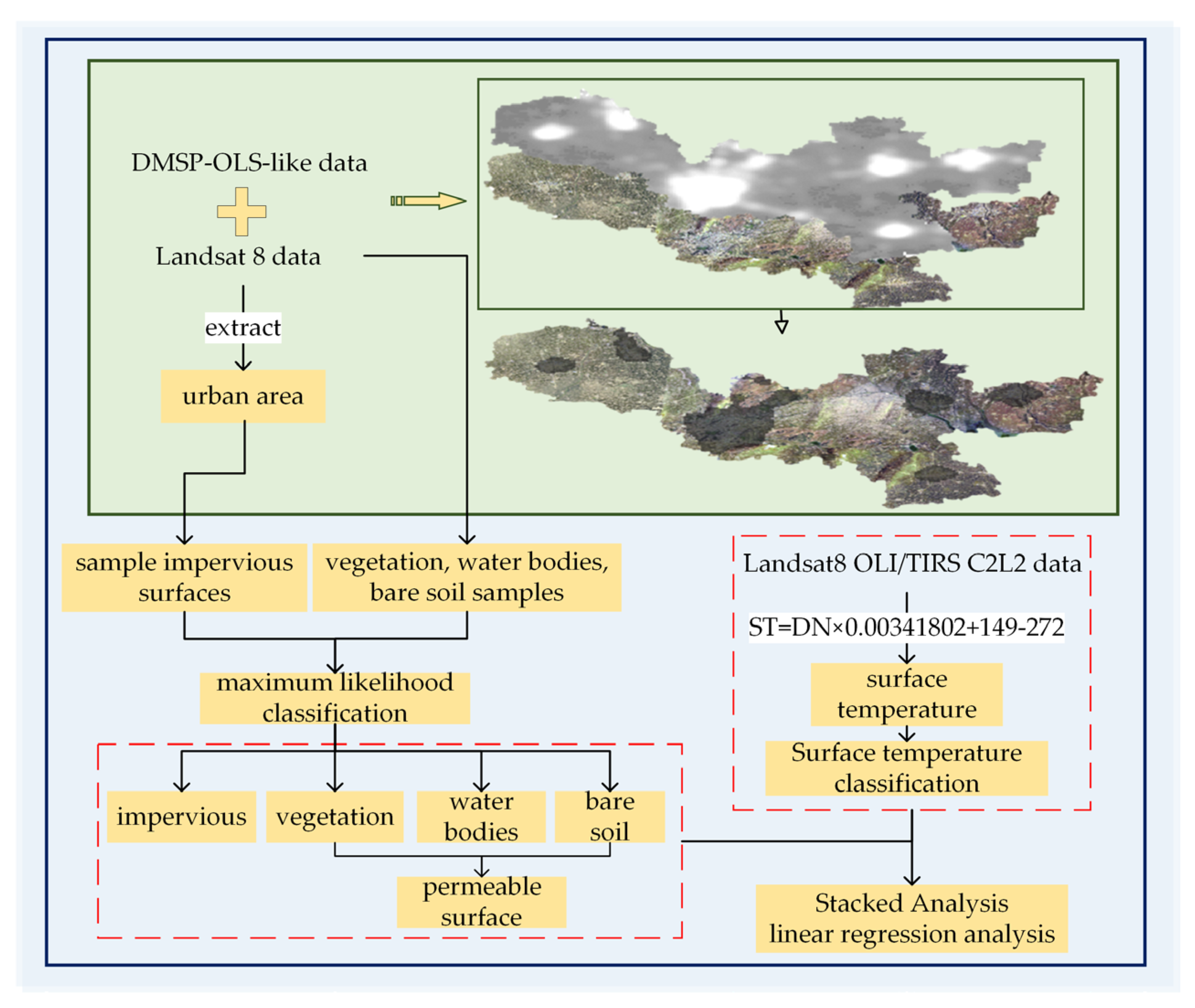
Figure 2.
Overview of the Study Area.
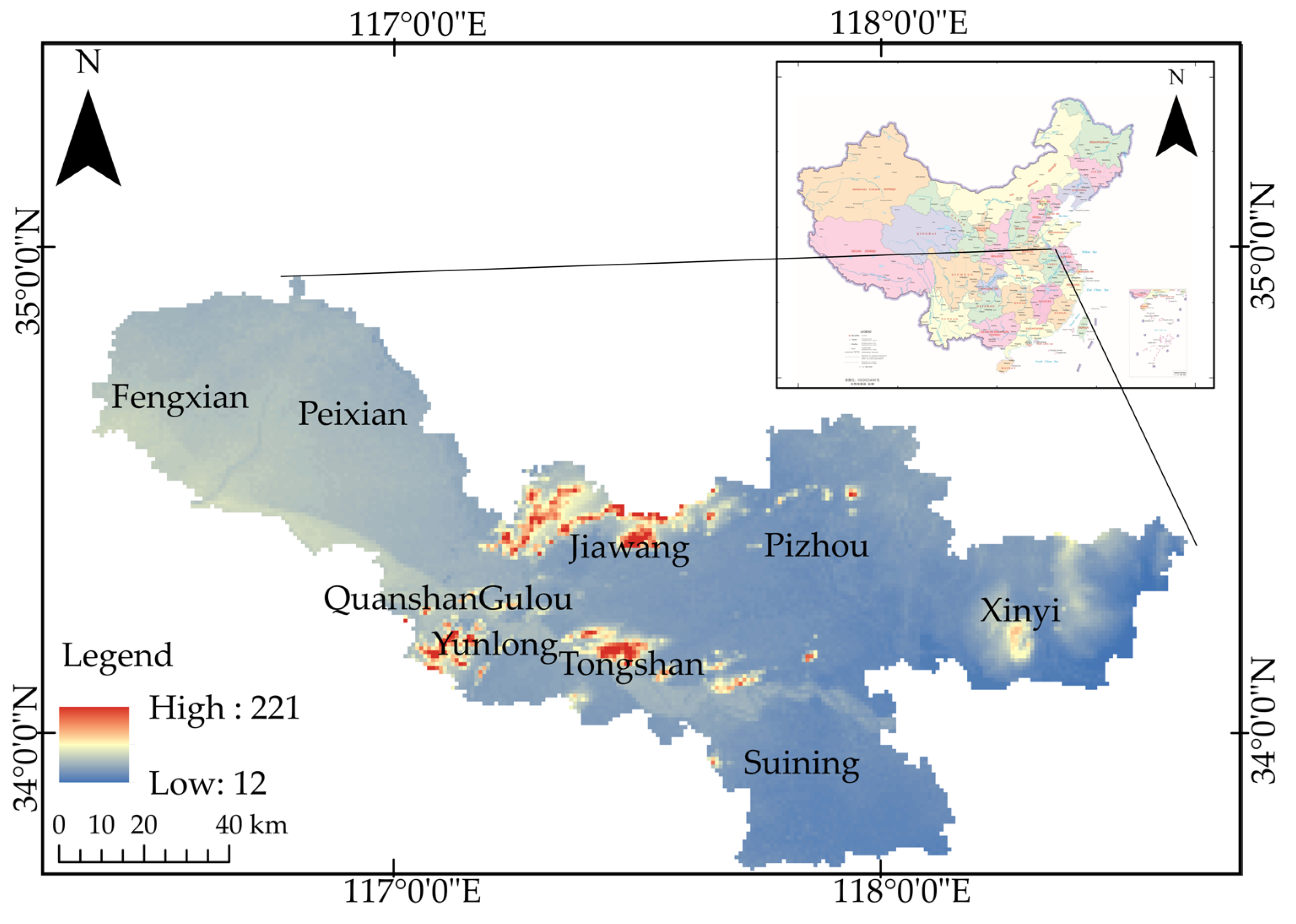
Figure 3.
The Distribution of Impervious Surface in Xuzhou City from 2013 to 2022.
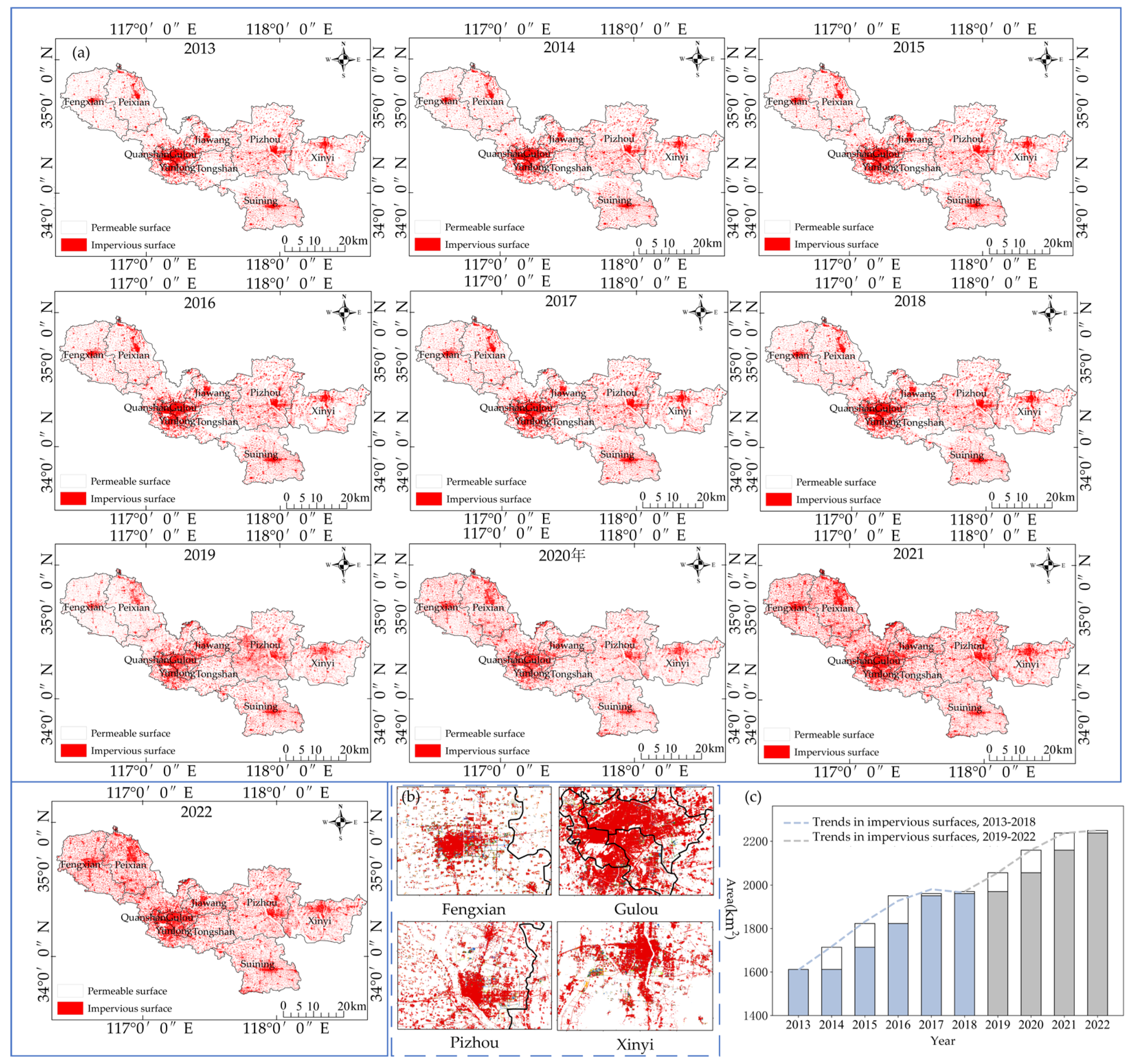
Figure 4.
(a) Comparison of Temperature Classification and Impervious Surface Areas in 2013 (b) Regression Analysis of Impermeable Surface Density and Average Temperature.
Figure 4.
(a) Comparison of Temperature Classification and Impervious Surface Areas in 2013 (b) Regression Analysis of Impermeable Surface Density and Average Temperature.
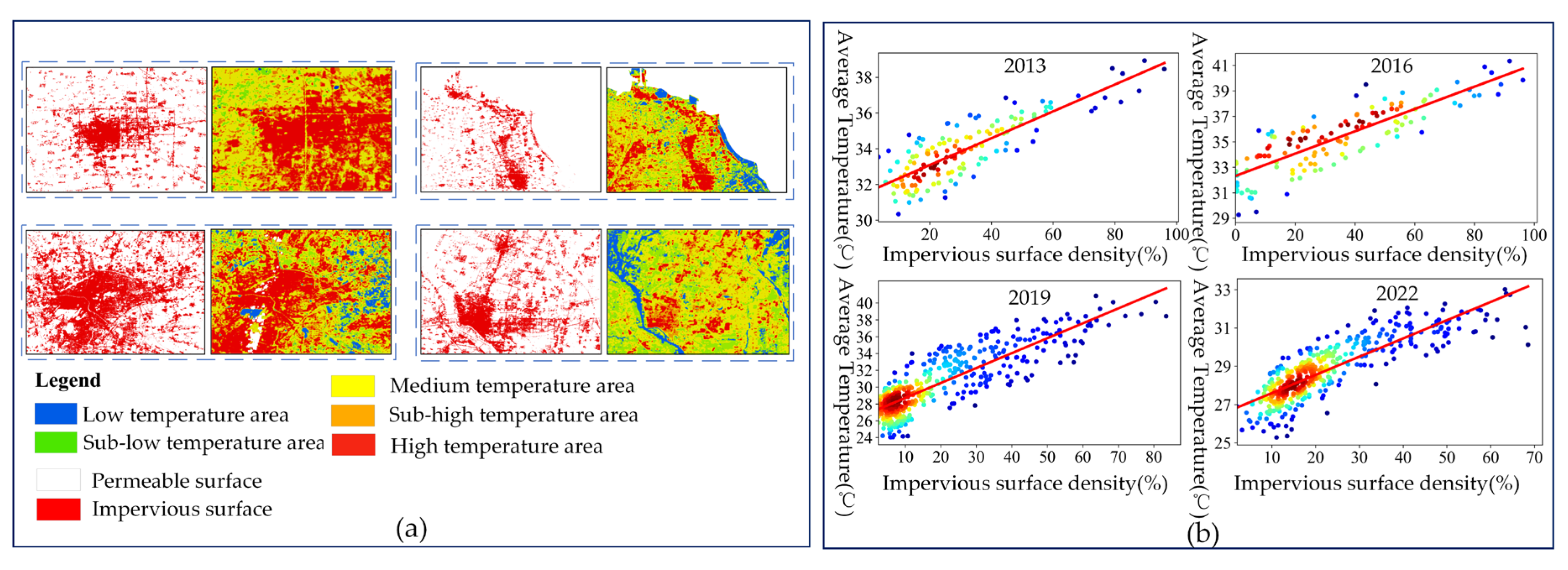

Table 1.
2013-2022 Impervious Surface Extraction Accuracy
| Year | User Accuracy | Kappa |
|---|---|---|
| 2013 | 97.80% | 0.8562 |
| 2014 | 97.79% | 0.8660 |
| 2015 | 97.81% | 0.8851 |
| 2016 | 97.75% | 0.8951 |
| 2017 | 97.76% | 0.8991 |
| 2018 | 97.77% | 0.9025 |
| 2019 | 94.74% | 0.8460 |
| 2020 | 92.08% | 0.8867 |
| 2021 | 93.23% | 0.9109 |
| 2022 | 95.28% | 0.9127 |
Table 2.
Table of Temperature Classifications.
| Temperature Classification Rules | |
|---|---|
| Lower temperature | Un<Um-Us |
| Subcooled zone | Um-Us<Un<Um-0.5×Us |
| Central temperature area | Un-0.5×Us<Un<Um+0.5×Us |
| Subtropical region | Um+0.5×Us<Un<Um+Us |
| High-temperature zone | Un>Um+Us |
Table 3.
Classification of Temperature of Impervious Surface from 2013 to 2022.
| Percentage of Impervious Surface Area by Temperature Classification, Xuzhou City, 2013-2018 | ||||||||||
|---|---|---|---|---|---|---|---|---|---|---|
| 2013 | 2014 | 2015 | 2016 | 2017 | 2018 | 2019 | 2020 | 2021 | 2022 | |
| Low temperature | 2.2% | 1.7% | 1.8% | 11.4% | 7.7% | 3.9% | 4.5% | 3.1% | 6.9% | 1.6% |
| Sub-low temperature | 3.4% | 5.4% | 7.0% | 6.1% | 6.0% | 8.0% | 4.4% | 6.1% | 9.4% | 3.5% |
| Medium temperature | 33.0% | 34.7% | 38.7% | 22.6% | 29.5% | 29.0% | 29.1% | 36.8% | 28.9% | 34.8% |
| Sub-high temperature | 21.1% | 21.2% | 22.2% | 15.0% | 23.0% | 21.8% | 26.9% | 27.3% | 17.4% | 28.7% |
| High-temperature | 40.2% | 36.9% | 30.0% | 44.8% | 33.8% | 37.3% | 35.0% | 26.7% | 37.5% | 31.4% |
Table 4.
Average Temperature of Xuzhou City from 2013 to 2022.
| Zonal average temperature 2013-2022 (℃) | |||
|---|---|---|---|
| year | Impervious Surface Aggregation Zone | Other impervious surface areas | permeable surface area |
| 2013 | 37.11 | 34.46 | 32.64 |
| 2014 | 31.90 | 30.23 | 28.90 |
| 2015 | 38.54 | 36.02 | 34.57 |
| 2016 | 37.34 | 34.06 | 31.85 |
| 2017 | 36.13 | 34.09 | 32.17 |
| 2018 | 34.30 | 32.20 | 30.10 |
| 2019 | 37.30 | 34.68 | 31.14 |
| 2020 | 30.58 | 29.61 | 27.91 |
| 2021 | 40.23 | 37.62 | 35.48 |
| 2022 | 32.60 | 30.44 | 28.49 |
Disclaimer/Publisher’s Note: The statements, opinions and data contained in all publications are solely those of the individual author(s) and contributor(s) and not of MDPI and/or the editor(s). MDPI and/or the editor(s) disclaim responsibility for any injury to people or property resulting from any ideas, methods, instructions or products referred to in the content. |
© 2024 by the authors. Licensee MDPI, Basel, Switzerland. This article is an open access article distributed under the terms and conditions of the Creative Commons Attribution (CC BY) license (http://creativecommons.org/licenses/by/4.0/).
Copyright: This open access article is published under a Creative Commons CC BY 4.0 license, which permit the free download, distribution, and reuse, provided that the author and preprint are cited in any reuse.


