Submitted:
09 October 2024
Posted:
10 October 2024
You are already at the latest version
Preprints on COVID-19 and SARS-CoV-2
Abstract
The COVID-19-induced strain on global supply chains led to significant market imbalances and unprecedented inflation, particularly affecting urban economies. Containment policies and stimulus packages resulted in unpredictable demand shifts, challenging urban supply chain planning and resource distribution. These disruptions underscored the need for robust risk management models, especially in cities where economic activity and population density exacerbate supply chain vulnerabilities. This study develops a comprehensive risk model tailored for G-7 urban economies, analyzing the causal and cointegration relationships between key economic indicators. Using Granger causality tests and a factor-augmented vector autoregression (FAVAR) approach, the study examines complex time series and high-dimensional variables, focusing on urban-specific indicators such as the Composite Leading Indicator (CLI) and Business Confidence Indicator (BCI). Our results indicate strong causal relationships among these indicators, validating CLI as a reliable early predictor of urban economic trends. The findings confirm the viability of this urban supply chain risk management model, offering potential pathways for strengthening urban resilience and economic sustainability in the face of future disruptions. This approach positions the study within the context of urban science, emphasizing the impacts on cities and how urban economies can benefit from the developed risk model.
Keywords:
supply chain risk
; VAR
; FAVAR
; causality analysis
1. Introduction
The global business landscape, facing constant threats from disruptions like the ongoing Covid-19 pandemic, grapples with supply chain challenges—shortages, financial losses, and demand-supply imbalances. Proactive risk mitigation, through strategic risk analysis and resilient supply chain development, is crucial. Learning from past disruptions is vital, necessitating companies to analyze incidents for enhanced resilience. Governments collaborate with businesses to formulate effective risk management plans, emphasizing the importance of seamless public-private sector collaboration. During crises, governments implement varying stimulus packages, underscoring the need for careful planning to prevent supply-demand imbalances and inflation.
To address these challenges, it is vital to classify disruptions based on their origin, such as supply-side, demand-side, or logistics-side disruptions [1]. Various external events can disrupt supply chains, including environmental, geopolitical, economic, and technological factors. In light of these challenges, this paper aims to propose a comprehensive model addressing various components simultaneously. This model considers the interdependencies among varied factors affecting supply chains. Additionally, the paper incorporates econometric analysis to study the relationships between the model components. By developing a comprehensive approach, this research contributes to the understanding of supply chain vulnerabilities and resilience strategies in the face of disruptions.
To tackle challenges effectively, it is crucial to categorize disruptions by their origin—supply-side, demand-side, or logistics-side [1]. Supply chains face disruptions from diverse external events, spanning environmental, geopolitical, economic, and technological factors. This paper proposes a holistic model addressing multiple components concurrently, recognizing the interdependencies among factors affecting supply chains. Utilizing econometric analysis, the paper explores relationships between model components. Through this comprehensive approach, the research enhances understanding of supply chain vulnerabilities and resilience strategies amid disruptions.
Supply chain disruptions, particularly during global crises like the COVID-19 pandemic, have profound effects on economic stability, especially in urban centers where economic activity is concentrated [2]. Urban economies are more vulnerable to disruptions due to their dependence on global supply chains for goods and services [3]. Previous research highlights the challenges faced by urban areas in managing supply chain risks, exacerbated by population density and logistical constraints [4], pointing out the importance of integrating sustainable practices and urban planning principles to enhance transportation security and supply chain efficiency within urban environments amid global disruptions [5].
Risk management models have increasingly focused on supply chain resilience, emphasizing the importance of real-time data, early warning indicators, and adaptive strategies [6]. Studies on the role of government policies, such as stimulus packages and containment measures, reveal their unintended consequences on supply chains, further complicating risk management efforts [7]. The integration of advanced econometric models, such as Granger causality and factor-augmented vector autoregression (FAVAR), provides valuable insights into the dynamic relationships between economic indicators, helping to predict and mitigate future disruptions [8].
While much of the literature addresses national and global scales, fewer studies focus on urban-specific challenges, particularly regarding how city-level economies respond to supply chain shocks. This paper addresses this gap by developing a comprehensive supply chain risk management model, tailored to urban economies in G-7 countries, using key indicators like the Composite Leading Indicator (CLI) and Business Confidence Indicator (BCI) as predictors of urban economic movements.
2. Materials and Methods
2.1. Supply Chain Risk Management Model
Business and government leaders have rarely faced with such a dynamic and complex set of volatile conditions in a number of fields simultaneously. This fact creates the necessity to develop a model to help decision-makers design supply chain resilience strategies considering many interrelated factors. Within the scope of this methodology, following research question needs to be answered:
Research Question: What is the causal relationship between Supply Chain Resiliency, Economic Environment, Risk Management, and Infrastructure?
Figure 1 depicts the framework developed to in this study to illustrate the complex environment in which decision-makers have to operate while overcoming supply chains challenges in the face of amid disruptors.
Effective supply chain risk management involves predicting and preventing incidents, addressing risk quantification, information sharing, and enhancing security. Economic policies and government responses add uncertainty, integral to risk models. External shocks, like pandemics, underscore the need for preparedness and integrated risk management. Proactive policies targeting supply chain resilience are crucial. Assessing causality relations among model factors in Figure 1 is critical. This study employs a Granger causality test and a factor-augmented vector autoregression (FAVAR) for nuanced detection of nonlinear, high-order causality and simultaneous analysis of direction and dynamic connectedness.
To assess the relationships among the model factors, Vector AutoRegression (VAR) in level and VAR in difference models are utilized for cointegration and causality analysis. VAR model can be expressed as below:
The classical VAR model becomes challenging even with moderately large dimensions (N and P) [9]. To draw inferences from the high-dimensional VAR model, limiting the parameter space (Eq. 1) to a feasible number of degrees of freedom is essential. However, time-series data exhibit significant temporal and cross-sectional dependency, impacting the accuracy of regularized estimation. To mitigate this, reducing the dimensionality of the model (Eq. 1) is essential. In this study, we implement a factor-augmented method for dimensionality reduction.
2.2. TVP-Factor-Augmented Vector Autoregression (FAVAR)
In FAVAR, observable and unobservable factors follow a vector autoregressive process, driving the co-movement of numerous observable variables [10,11]. This method addresses the omitted variable problem and enables the estimation of internally consistent Structural Impulse Response Functions (SIRFs) for a wide range of variables.
Researchers have utilized FAVAR in assorted studies. Ramsauer et al. (2019) extended FAVAR to mixed frequency and incomplete panel data, measuring the monetary policy impact on financial markets and the real economy [12]. Wang et al. (2017) used FAVAR with stochastic volatility and time-varying coefficients to create a financial conditions index, analyzing the relationship between future inflation and a composite index of financial indicators [13]. Vargas-Silva (2008) explored the relationship between monetary policy and the housing market using impulse response functions obtained from a FAVAR model [14].
In this study, for the slow-R-fast scheme, certain assumptions are made: COVID-19 effect or news/financial shocks do not immediately affect slow-moving variables such as long-term interest rates, employment, and trade in goods within a given period. Fast-moving variables, such as industrial production and consumer confidence indicators, respond to all types of shocks, including COVID-19 shocks, which are reflected solely in these variables. If multivariate stochastic volatilities are allowed to exist on the factors, then we have a FAVAR model.
The FAVAR model [9] describes the relationship between the observed variables , the unobserved factors , and the observable economic variables
The model captures the relationship between , , and through lagged relationships represented by . The factors summarize additional economic information not fully captured by the observable variables . The matrices and capture how these factors and observable variables contribute to the observed variables . The model allows for a richer representation of the underlying economic dynamics by incorporating unobserved factors , making it more flexible than traditional VAR models based solely on observable variables .
3. Empirical Findings
3.1. Data
Cross-country data obtained from the OECD database from February 2010 to September 2022 are used to investigate the causality and cointegration between the factors of the supply chain risk model explained below. Table 1 summarizes the indicators and their explanations for the data spanning 56 dimensions.
3.2. Results
This section initiates by illustrating the causal relationships among the indicators listed in Table 1. The model summary for G7 countries is detailed in Table 2, while country-level causality relationships are available as supplementary files.
Results reveal robust two-way relationships among the Unemployment Rate, Producer Price Indices, and Trade in Goods at a 1% significant level. Similarly, a significant correlation exists between the Consumer Confidence Indicator and Business Confidence Indicator. Notably, a causal relationship emerges between Trade in Goods, Unemployment Rate, and Composite Leading Indicator at a 5% significance level.
A concise summary of the empirical findings regarding the indicators’ effects on the FAVAR model is presented below. For detailed results, refer to Table 3 and Table 4, which summarize the estimation results for three and four factors, respectively, with comprehensive details available in the supplementary materials.
Three dimensions explain the variation in BCI, CCI, CLI, HUR, PPI, and TRG with extremely high significance (p-values < 2.2e-16 for all equations). The R² values for all equations are very high, ranging from 0.9409 for TRG to 0.9975 for CCI. This suggests that the three-factor model captures most of the variance in these economic indicators leading to the conclusion that a three-factor FAVAR model effectively captures the dynamics of the indicators with excellent explanatory power across the board.
Table 4 shows that adding a fourth factor slightly reduces the explanatory power for some variables, particularly for Dimension 4 (R² = 0.8824) and TRG (R² = 0.9362). While the p-values remain highly significant across all factors and indicators, some degradation in fit occurs compared to the three-factor model, showing that the four-factor model leads to marginal improvements in fit for certain indicators (e.g., CCI and BCI), but overall, the three-factor model provides a more effective explanation.
Figure 2 displays the scree plot, illustrating the variation captured by each principal component from the data. The percentages indicate three factors (>10%) for the FAVAR model, while the “elbow” rule suggests four factors.
Figure 3 depicts the trends of the three and four factors, revealing the adverse effects of the 2020 COVID-19 pandemic, marked by a deep V shape occurring from January to June 2020.
Figure 4 and Figure 5 show Impulse Response Functions (IRFs) and Response figures for three factors.
Figure 6 and Figure 7 present IRFs and Response figures for four factors from the FAVAR model, respectively. Figure 6 suggests the presence of a singular dynamic factor that translates into three distinct static factors. These factors respond to various structural shocks, and their reactions to these shocks differ significantly. This structural instability might result in the generation of excessively numerous static factors, potentially leading to misleading conclusions or interpretations in the analysis.
4. Discussion and Conclusions
The results show that past values of economic indicators, especially BCI, CCI, HUR, and PPI, play crucial roles in predicting future movements. The three-factor FAVAR model offers a highly effective explanation of the dynamics of these indicators, with near-perfect fit (R² values exceeding 0.95 for most indicators). Adding a fourth factor adds complexity without significant improvement. This analysis suggests that economic confidence, unemployment rates, and price indices are tightly interconnected, and understanding their historical data helps forecast future trends effectively.
This study introduces a comprehensive model incorporating supply chain disruption indicators and response capabilities, including those of governments. Faced with the challenges of high-dimensional data in supply chain modeling and the limitations of conventional economic theory models, we employ a Granger causality test and a FAVAR model for empirical analysis, enhancing the traditional state-space model VAR. Utilizing a dataset spanning 2010 to 2022 with 8 variables for G-7 countries, the FAVAR model explores relationships amid external shocks, bridging data-driven empirical models with theoretical frameworks and advancing our understanding of economic dynamics.
The proposed supply chain risk management model, grounded in economic and management theories, is validated through Granger tests and the FAVAR model. While the empirical results affirm the model’s viability, further research avenues are identified. Future studies may expand the model by incorporating additional indicators related to risk management policies, external factors, infrastructure, economic environment, government response, and supply chain resilience. Additionally, extending the research scope to include diverse global regions would allow for testing the model on countries with varying economic, political, and environmental characteristics.
Author Contributions
Conceptualization, H.W. and L.S.; methodology, H.W.; software, H.W.; validation, H.W. and L.S.; formal analysis, H.W.; investigation, L.S.; resources, L.S.; data curation, L.S.; writing—original draft preparation, L.S.; writing—review and editing, H.W. and L.S.; visualization, H.W.; supervision, H.W. All authors have read and agreed to the published version of the manuscript.
Funding
This research received no external funding.
Data Availability Statement
Data will be made available by the authors upon reasonable request.
Conflicts of Interest
The authors declare no conflicts of interest.
References
- Raj, A.; Mukherjee, A.A.; Jabbour, A.B.L.d.S.; Srivastava, S.K. Supply chain management during and post-COVID-19 pandemic: Mitigation strategies and practical lessons learned. J. Bus. Res. 2022, 142, 1125–1139. [Google Scholar] [CrossRef]
- Ivanov, D. 2020. Predicting the impacts of epidemic outbreaks on global supply chains: A simulation-based analysis on the coronavirus outbreak (COVID-19/SARS-CoV-2) case. Transportation Research Part E: Logistics and Transportation Review.
- Sarkis, J.; Cohen, M.J.; Dewick, P.; Schröder, P. A brave new world: Lessons from the COVID-19 pandemic for transitioning to sustainable supply and production. Resour. Conserv. Recycl. 2020, 159, 104894–104894. [Google Scholar] [CrossRef]
- Turoff, M. , Chumer, M., Van de Walle, B., & Yao, X. 2013. Emergency planning as a continuous process. International Journal of Information Systems for Crisis Response and Management.
- Jinor, E.; Bridgelall, R. Bibliometric Insights into Balancing Efficiency and Security in Urban Supply Chains. Urban Sci. 2024, 8, 100. [Google Scholar] [CrossRef]
- Tang, C. S. 2006. Perspectives in supply chain risk management. International Journal of Production Economics.
- Dolgui, A. , & Ivanov, D. 2021. Ripple effect in supply chains: Definitions, frameworks and future research perspectives. Annals of Operations Research.
- Stock, J.H.; Watson, M.W. Forecasting Using Principal Components From a Large Number of Predictors. J. Am. Stat. Assoc. 2002, 97, 1167–1179. [Google Scholar] [CrossRef]
- Krampe, J.; Paparoditis, E.; Trenkler, C. Structural inference in sparse high-dimensional vector autoregressions. J. Econ. 2022, 234, 276–300. [Google Scholar] [CrossRef]
- Bernanke, B. S. , Boivin, J., and Eliasz, P. 2005. “Measuring the Effects of Monetary Policy: A Factor-Augmented Vector Autoregressive (FAVAR) Approach.” The Quarterly Journal of Economics, 120(1): 387–422.
- Bai, J.; Li, K.; Lu, L. Estimation and Inference of FAVAR Models. J. Bus. Econ. Stat. 2016, 34, 620–641. [Google Scholar] [CrossRef]
- Ramsauer, F.; Min, A.; Lingauer, M. Estimation of FAVAR Models for Incomplete Data with a Kalman Filter for Factors with Observable Components. Econometrics 2019, 7, 31. [Google Scholar] [CrossRef]
- Wang, S.; Xu, F.; Chen, S. Constructing a dynamic financial conditions indexes by TVP-FAVAR model. Appl. Econ. Lett. 2018, 25, 183–186. [Google Scholar] [CrossRef]
- Vargas-Silva, C. The effect of monetary policy on housing: a factor-augmented vector autoregression (FAVAR) approach. Appl. Econ. Lett. 2008, 15, 749–752. [Google Scholar] [CrossRef]
Figure 1.
Supply chain risk management model.

Figure 2.
Scree Plot of Factor Analysis.
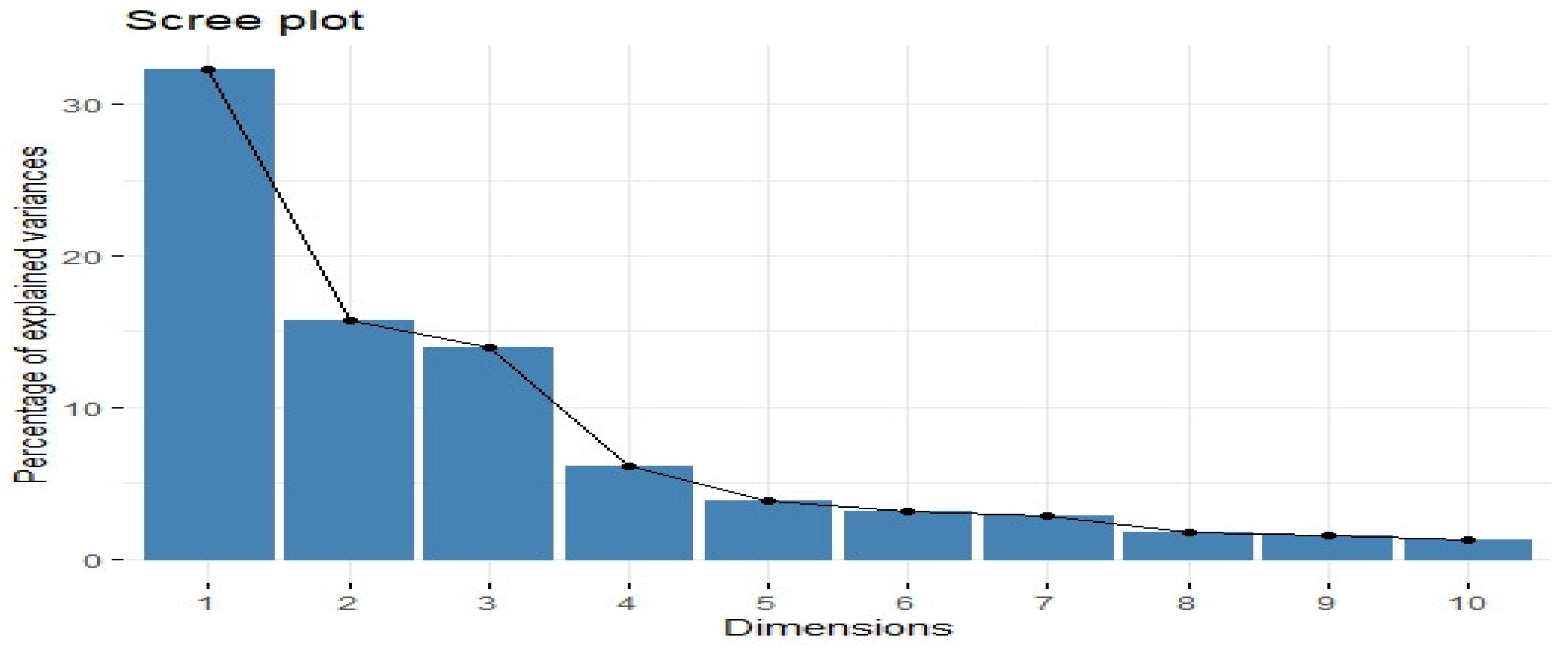
Figure 3.
Density plots of Factors.
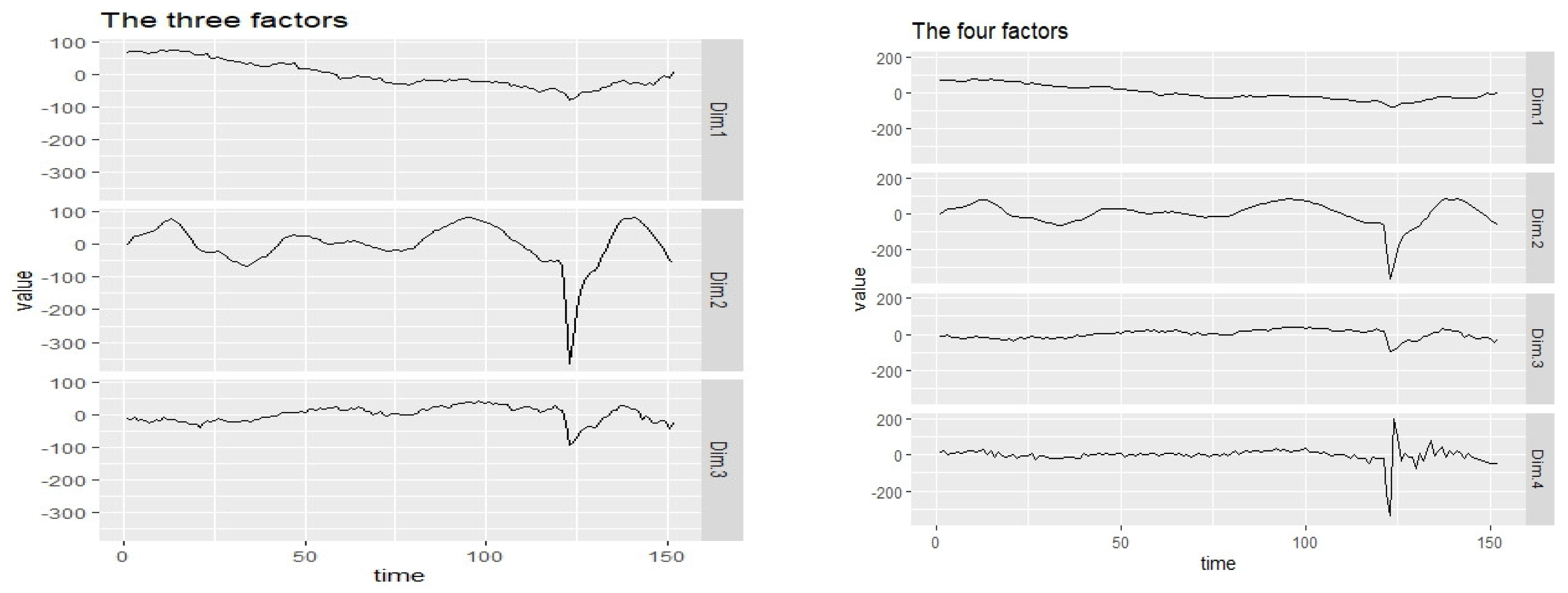
Figure 4.
Three-factor IRFs of variables.
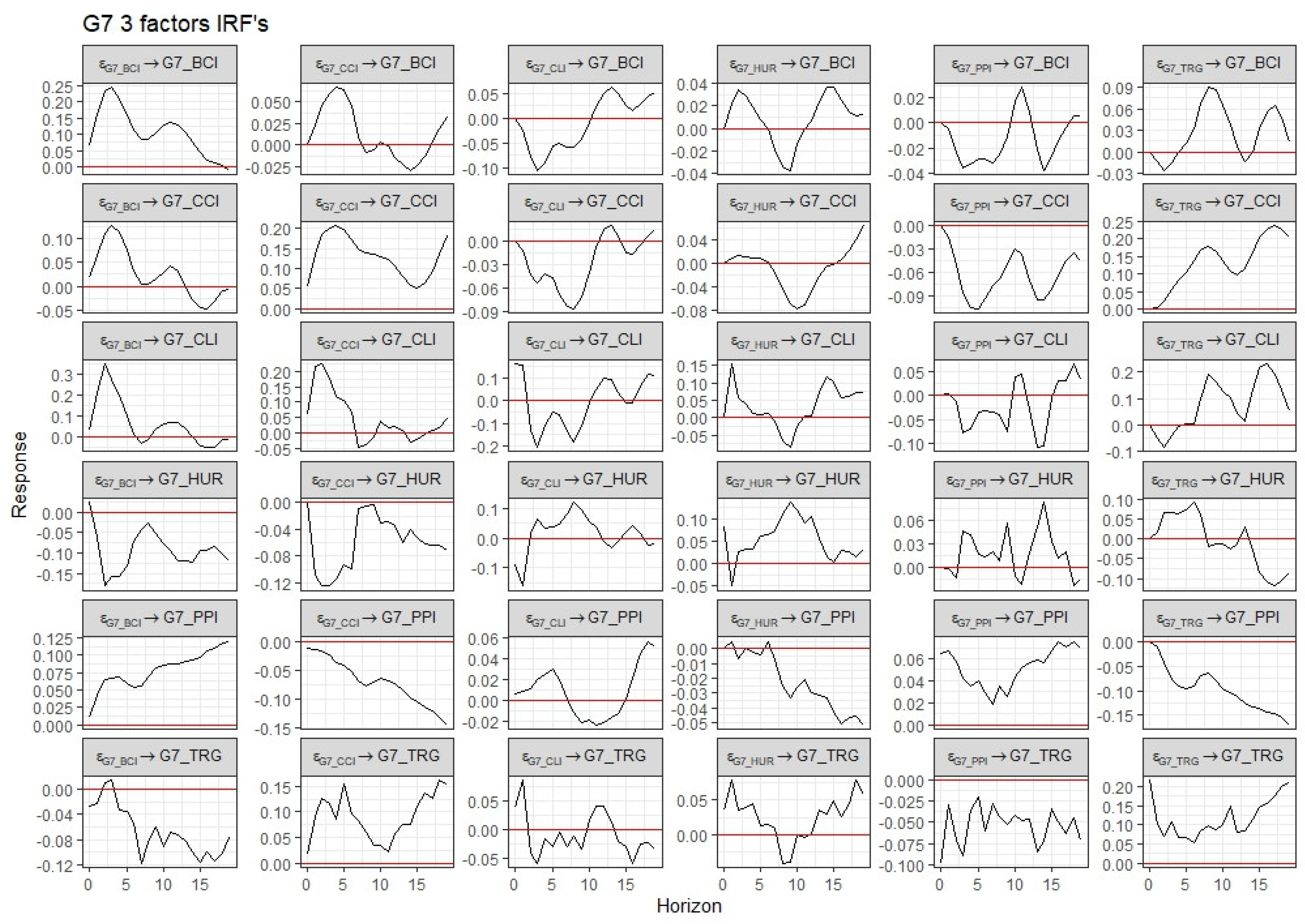
Figure 5.
Three-factor response of variables.
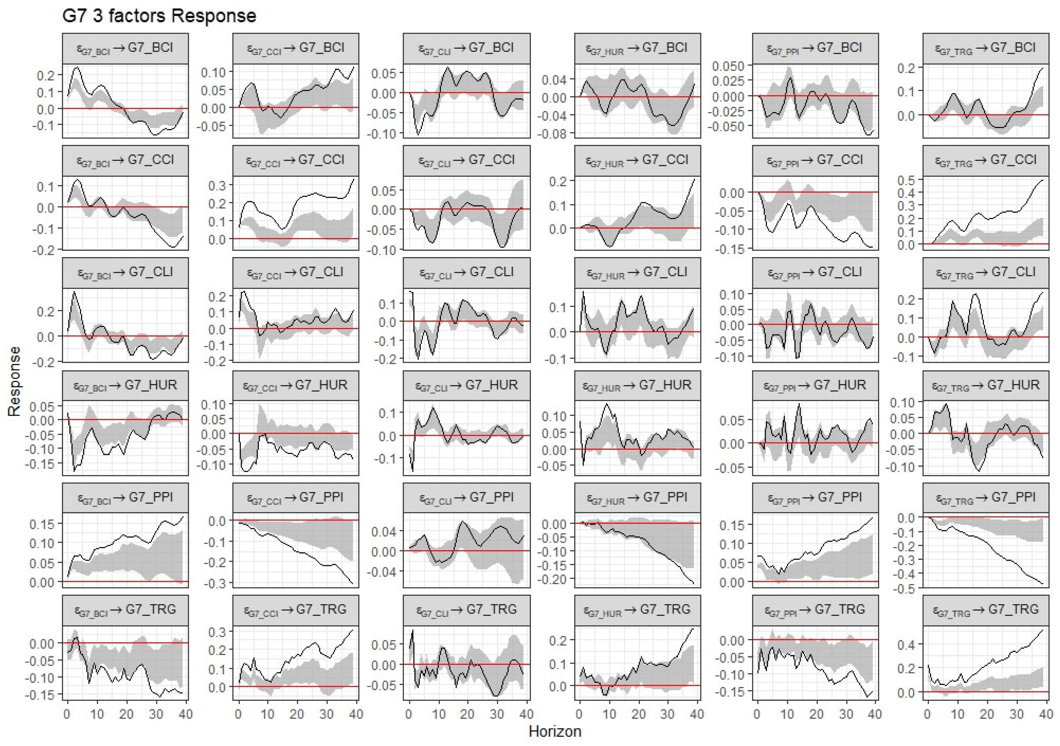
Figure 6.
Four-factor IRFs of variables.
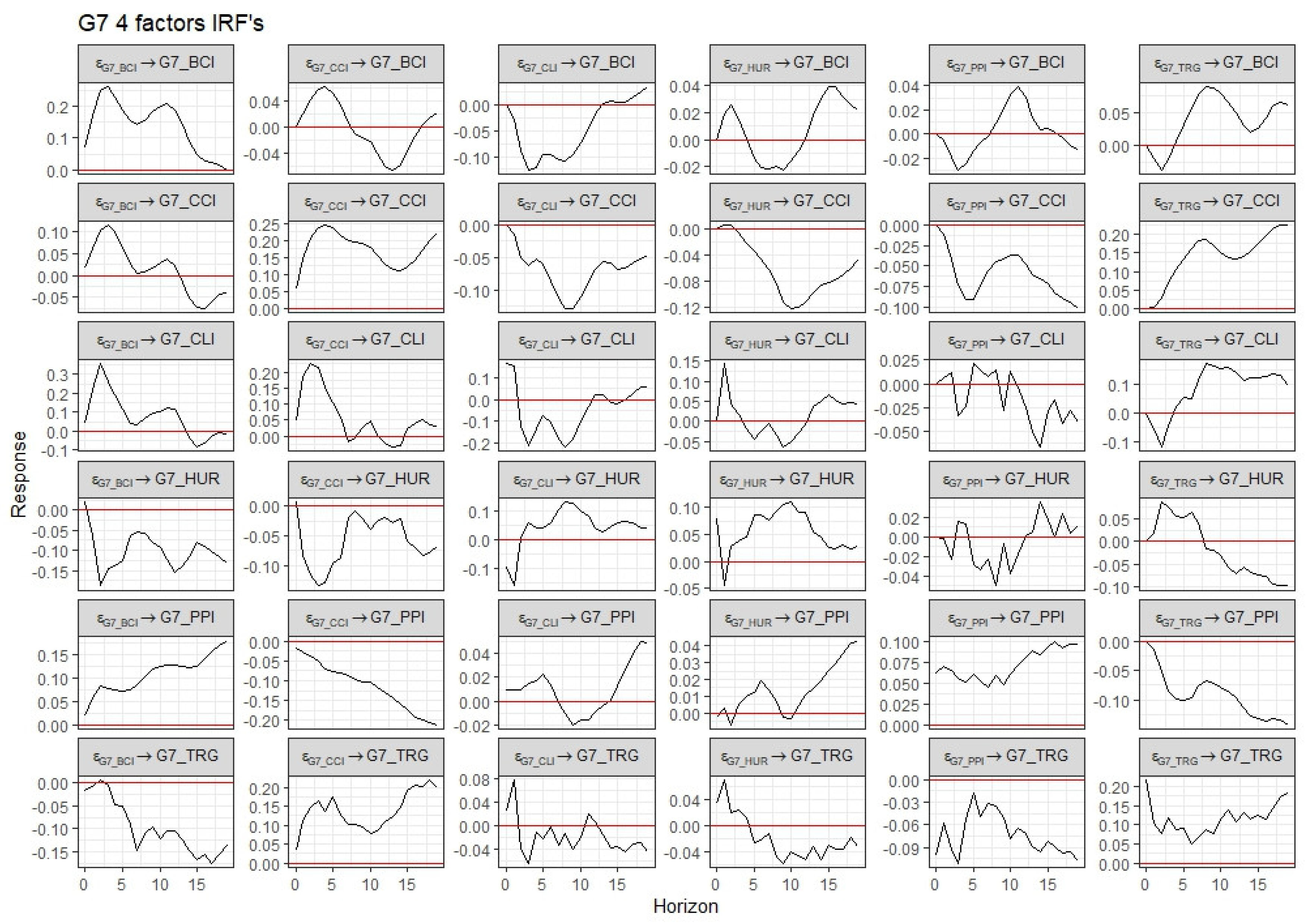
Figure 7.
Four-factor response of variables.
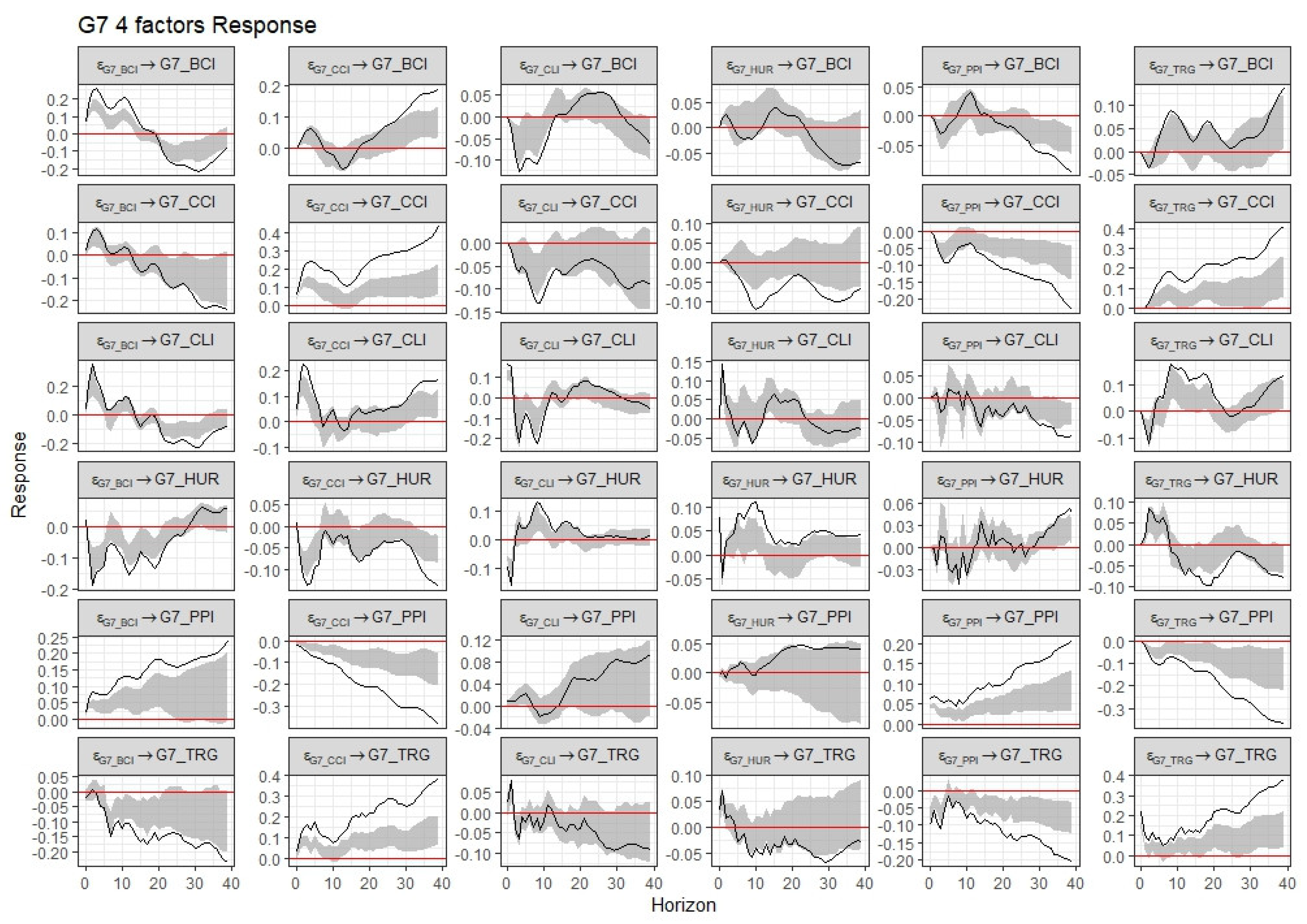

Table 1.
Summary of Indicators.
| Explanation | Measurement | |
|---|---|---|
| Industrial production (IP) | Output of industrial establishments. | Change in volume of production output |
| Unemployment (HUR) | Provides an indication of the economic activity. | Number of unemployed people as a percentage of the workforce |
| Composite leading indicator (CLI) | Provides early signs of future economic movements. | Amplitude adjusted. |
| Business confidence indicator (BCI) | Provides insights about future expectations of businesses, measured by surveys. | BCI > 100 suggests an increased confidence in business performance. |
| Consumer confidence indicator (CCI) | An indication of how consumers feel about their future financial situation. | CCI > 100 indicates an increase in confidence in the future financial situation. |
| Long-term interest rate | Government bonds maturing in 10 years. | Averages of daily rates, measured as a percentage |
| Producer price indices (PPI) | Measures the rate of change in product prices as they leave the producer. | Measured in terms of the annual growth rate and index. |
| Trade in goods (TRG) | All goods which add to or subtract from the stock of material resources of a country through exports or imports. | Measured in million USD |
Table 2.
Model Summary.
| BCI | CCI | CLI | HUR | PPI | TRG | |
|---|---|---|---|---|---|---|
| BCI.l1 | (0.166)*** | (0.185)*** | (0.249)* | (0.212)*** | ||
| CCI.l1 | (0.140)*** | (0.210)** | ||||
| CLI.l1 | (0.150)* | |||||
| HUR.l1 | -1.001*** | -3.589*** | ||||
| PPI.l1 | (0.037)* | (0.228)*** | (0.818)*** | |||
| TRG.l1 | (0.010)** | (0.051)*** | (0.183)*** | |||
| BCI.l2 | (0.169)*** | (0.253)* | ||||
| CCI.l2 | ||||||
| CLI.l2 | (0.919)* | -3.293** | ||||
| HUR.l2 | (0.165)*** | (0.184)** | (0.247)*** | |||
| PPI.l2 | (0.034)*** | (0.038)** | (0.052)*** | |||
| TRG.l2 | (0.008)*** | (0.012)** | ||||
| BCI.l3 | -1.155* | |||||
| CCI.l3 | ||||||
| CLI.l3 | (0.127)** | (0.141)* | (0.190)* | (0.862)* | ||
| HUR.l3 | (0.135)*** | (0.150)*** | (0.202)*** | (0.915)** | -3.280* | |
| PPI.l3 | (0.037)* | |||||
| TRG.l3 | ||||||
| const | -31.456*** | -47.133*** | -40.145* | |||
| R2 | 0.626 | 0.755 | 0.492 | 0.739 | 0.765 | 0.713 |
| Adj. R2 | 0.574 | 0.721 | 0.422 | 0.702 | 0.733 | 0.673 |
p values. *** at 1%, **at 5%, and*at 10% levels of significance.
Table 3.
FAVAR Estimation Results for Three Factors.
| Equation | Dim.1 | Dim.2 | Dim.3 | G7_BCI | G7_CCI | G7_CLI | G7_HUR | G7_PPI | G7_TRG |
|---|---|---|---|---|---|---|---|---|---|
| p-value | < 2.2e-16 | < 2.2e-16 | < 2.2e-16 | < 2.2e-16 | < 2.2e-16 | < 2.2e-16 | < 2.2e-16 | < 2.2e-16 | < 2.2e-16 |
| R2 | 0.9922 | 0.9794 | 0.9521 | 0.9958 | 0.9975 | 0.9816 | 0.989 | 0.9967 | 0.9409 |
Table 4.
FAVAR Estimation Results for Four Factors.
| Equation | Dim.1 | Dim.2 | Dim.3 | Dim.4 | G7_BCI | G7_CCI | G7_CLI | G7_HUR | G7_PPI | G7_TRG |
|---|---|---|---|---|---|---|---|---|---|---|
| p-value | < 2.2e-16 | 2.37E-13 | 1.47E-10 | 5.03E-07 | < 2.2e-16 | < 2.2e-16 | 1.36E-14 | < 2.2e-16 | < 2.2e-16 | 2.22E-09 |
| R2 | 0.9923 | 0.9764 | 0.9527 | 0.8824 | 0.9961 | 0.9982 | 0.9826 | 0.9919 | 0.9978 | 0.9362 |
Disclaimer/Publisher’s Note: The statements, opinions and data contained in all publications are solely those of the individual author(s) and contributor(s) and not of MDPI and/or the editor(s). MDPI and/or the editor(s) disclaim responsibility for any injury to people or property resulting from any ideas, methods, instructions or products referred to in the content. |
© 2024 by the authors. Licensee MDPI, Basel, Switzerland. This article is an open access article distributed under the terms and conditions of the Creative Commons Attribution (CC BY) license (https://creativecommons.org/licenses/by/4.0/).
Copyright: This open access article is published under a Creative Commons CC BY 4.0 license, which permit the free download, distribution, and reuse, provided that the author and preprint are cited in any reuse.


