Analysis of the Intensity of Energy Consumption in the Transportation Sector of the Oil-Rich Country

1. Introduction

The increase in energy demand is driving economic expansion in nations. Simultaneously, constraints in existing energy sources and escalating environmental concerns arising from economic ventures have prompted planners and policymakers to focus on efficient energy consumption management. Following the energy crisis of the 1990s and the surge in energy costs, along with apprehensions regarding climate change, efforts to enhance energy consumption have become essential components of public policy discourse. Recognizing factors influencing variations in energy intensity and understanding the significance of energy efficiency are now crucial considerations for policymakers (Jimínez and Mercado1, 2014).

The concept of energy intensity is closely associated with energy efficiency, where energy intensity signifies the amount of energy required per unit of production, while energy efficiency improves when the same level of output is achieved with reduced energy consumption. As a result, energy intensity measurement serves as a common proxy for efficiency in the energy literature. Given the imperative of decreasing energy intensity to address mounting concerns regarding rising greenhouse gas emissions and energy security, examining historical trends and determinants across various countries can prove advantageous(Motafakerzadeh & Gholami, 2018). Evaluating the energy consumption intensity in Iran and juxtaposing it with other nations can highlight inefficiencies in energy utilization. The main goal of this research is to identify the factors that influence energy intensity in order to facilitate the implementation of effective control measures. Moreover, the study recognizes the significant role of the transportation sector in energy consumption and its impact on pollutant emissions. This study examines the factors that affect energy intensity and their environmental consequences (Azizi, 2014). The research comprehensively addresses the problem statement and rationale, delves into the theoretical and empirical background, scrutinizes the results of model estimation in the research methodology, and offers recommendations grounded in the findings. Transportation encompasses a range of activities about to the movement of people and goods within the economy, including various modes of transport such as rail, road, air, sea, pipelines, and associated services both domestically and internationally (Razmi & Azari, 2009). Classified according to its function in providing access to resources and markets, the expansion of transportation infrastructure facilitates the production and trade of goods, resulting in diminished transaction costs and ultimately culminating in heightened productivity. This rise in productivity and cost reduction has the potential to lower overall production costs. Data indicates that the transportation sector’s contribution to GDP declined from 2.5% in 1959 to 1.3% in 1969 but has since witnessed a consistent increase, now standing at 8.7% annually (Azizi & Jabbari, 2024).

Figure 1. Share Each Products oil And gas style At the part carry And quote At Year2011. Source: balance sheet Energy country Year2012.

Figure 1. Share Each Products oil And gas style At the part carry And quote At Year2011. Source: balance sheet Energy country Year2012.

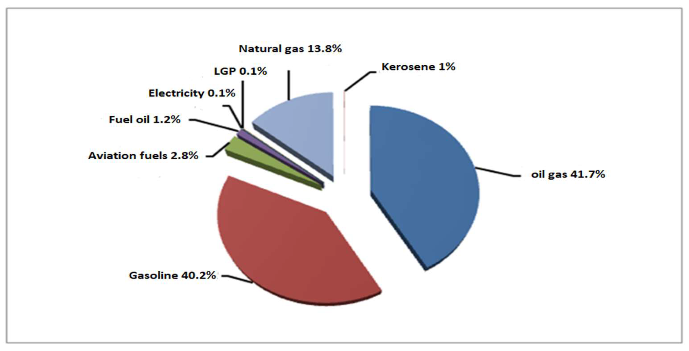
Whole consumption of final energy in the year 2011 is equivalent to 1227.3 million barrels of oil. This represents 24.23% of the total amount, which is equivalent to 297.37 million barrels of oil.

Figure 2. Share the part carry and quote From Consumption final energy At Year2011. Source: 2012 country’s energy balance sheet.

Figure 2. Share the part carry and quote From Consumption final energy At Year2011. Source: 2012 country’s energy balance sheet.

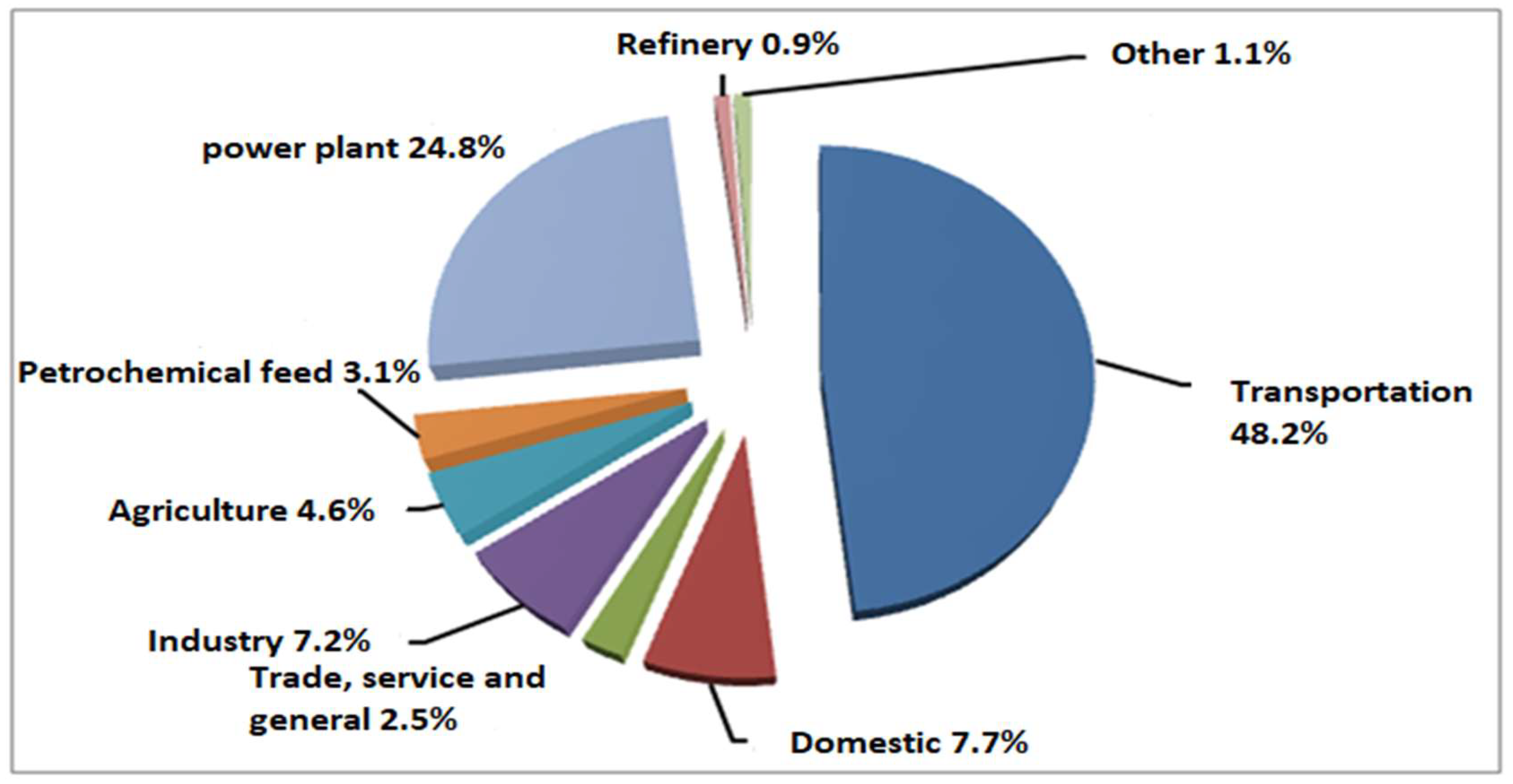
Considering the growing trend of energy consumption in the country and the high share of the transportation sector in this trend, identifying the drivers affecting energy consumption in this sector is of particular importance.

2. Theoretical and Experimental Background of the Research

In economic literature, production functions typically involve various inputs, and researchers often examine the unique characteristics of energy as an input compared to others. This differentiation of energy is emphasized in studies like Burnett and Wood’s research from 1979, which highlighted the weak separable relationship between energy and labor in the production process. They proposed a production function that encompasses this distinction (Taheri, et al. 2014). $Q=f\left[g\left(K,E\right),L\right]$ (1)

Sach and Brano conducted a study on the correlation between energy consumption and energy levels. They analyzed the impact of imported raw materials on the economy’s supply function, with a focus on the effects of rising oil prices. The general format of their proposed function is as follows: $Q=f\left[L,K,R\right]$ (2)

Within this framework, the variable Q is used as a representation of Gross Domestic Product (GDP) and is believed to be influenced by a variety of factors including service inputs capital K, labor L, and imported raw materials R. Each of these factors has both positive and negative effects on the production scale (Azizi, et al. 2011). The recent increase in oil prices has had a significant impact on the economies of a number of countries, underscoring the vital role that energy plays in production processes and the overall economic well-being of nations.

The noticeable shift to the left in the supply curve of economies in the Western world due to escalating energy costs further highlights the substantial influence that energy has on production activities and economic processes on a global scale. According to biophysical growth models outlined by Ayres and Nair, which draw upon the work of Stern, the production of goods within economic systems necessitates a significant amount of energy expenditure (Pongthanaisawan, 2010). Therefore, energy is the only and most important factor of growth, and labor and capital are intermediate factors that need energy to be employed ${\displaystyle \frac{\partial \mathrm{Q}}{\partial \mathrm{K}}}$> 0, > 0, > 0${\displaystyle \frac{\partial \mathrm{Q}}{\partial \mathrm{L}}}{\displaystyle \frac{\partial \mathrm{Q}}{\partial \mathrm{E}}}$.

Energy input can be provided by a set of factors such as oil, gas, electricity, coal, etc., which are known as carriers (Imam Vardi et al., 2012).

1.2. Energy Intensity and Factors Affecting It

Energy intensity serves as a critical indicator for evaluating the level of energy efficiency achieved in the economic structure of a nation. It is determined by dividing the final energy consumed by the gross domestic product, signifying the quantity of energy required to manufacture a particular volume of goods and services (Minhaj, et al. 2015). Several elements play a significant role in shaping the energy intensity of a country, such as the energy pricing, income status, technological progressions, quality of life, climatic conditions, and the industrial and economic composition. Typically, countries with elevated living standards exhibit increased energy utilization, consequently resulting in heightened levels of energy intensity (Energy balance sheet, 2013).

1.1.2. Relative Price of Energy

Pindyck (1979) Suggests that the influence of energy prices on economic growth depends on the function of energy within the production process. In sectors where energy is used as an intermediate input in production, an increase in energy prices (resulting in reduced energy consumption) is likely to hurt production capacity and output, leading to a decrease in overall national production levels.

Higher energy prices lead to changes in energy consumption patterns due to increased costs. Within a competitive market environment, elevated energy prices encourage the adoption and substitution of technologies that require greater labor and capital inputs. As a result, labor and capital productivity may decrease, while energy productivity increases. Conversely, lower energy prices incentivize the use of technologies with lower labor and capital requirements, leading to a decrease in energy productivity and an increase in labor and capital productivity (Sharifi, 2013). In a competitive market, it is expected that higher energy prices will drive the adoption of technologies with improved energy efficiency, while lower energy prices will favor technologies with lower energy efficiency. Therefore, an increase in energy prices is projected to contribute to a reduction in energy intensity (Adam, 2015).

2.1.2. Production Technology

According to theory, when the technology or productivity level of all production factors increases, fewer inputs are needed to produce a certain amount of product. This results in lower energy intensity. Technological advancements have improved the potential for enhancing energy efficiency, which will ultimately reduce energy intensity (Jamshidi, 2008).

3.1.2. Clean and Renewable Energies

With the limitations of fossil fuel reserves and the escalating global energy demand, depending on conventional energy sources is no longer viable in the present-day context. The emergence and rapid expansion of alternative energy sources like solar, wind, hydroelectric, biogas, and geothermal energy can be attributed to their accessibility, cost-effectiveness, environmental friendliness, and long-term sustainability. The escalation of environmental challenges has fueled substantial interest in these sustainable and cost-efficient energy options at both national and international levels (Seifipour & Afrooz, 2012). The establishment of the International Renewable Energy Agency in April 2010 was aimed at advancing the adoption, generation, and sustainable utilization of renewable energy, with a current membership of 85 countries and approximately 70 signatories. In 2010, global investments in renewable energy amounted to a landmark $211 billion, marking the first instance where more than half of this investment was directed towards developing nations (Zarei & Azizi, 2024).

3. Methodology

Creating a model to examine the variables impacting the level of energy usage in the transportation industry involves understanding the elements that influence the demand for products necessary in transportation. These factors can be categorized into economic, technical, environmental, and social factors based on existing theories. Economic factors include income levels, consumer preferences, and the price of fuel relative to other goods, as well as expectations for future prices and preferences.

The model utilized in this study is constructed using three main components: theoretical principles, empirical data from previous studies, and specific information pertaining to selected variables. The overall framework of the model can be summarized as follows (Salimfar & Rahimi, 2009):

$$\mathit{L}\mathit{n}{\left( \mathit{E}\mathit{I}\mathit{T}\right)}_{\mathit{t}}={\mathit{\alpha }}_0+{\mathit{\alpha }}_1\mathit{l}\mathit{n} {\left(\mathit{E}\mathit{P}\right)}_t+{\mathit{\alpha }}_2\mathit{l}\mathit{n} {\left(\mathit{K}\mathit{H}\mathit{O}\mathit{D}\right)}_{\mathit{t}}+{\mathit{\alpha }}_{3}ln {\left(\mathit{I}\mathit{T}\mathit{V}\mathit{T}\right)}_t+{\mathit{\alpha }}_4\mathit{l}\mathit{n} {\left(\mathit{P}\mathit{O}\mathit{P}\right)}_{\mathit{t}}+{\mathit{\alpha }}_5\mathit{l}\mathit{n} {\left(\mathit{C}\mathit{E}\right)}_{\mathit{t}}+{\epsilon }_t$$

Where in;

$\mathit{E}\mathit{I}\mathit{T}$: Energy intensity index of transportation sector

$\mathit{E}\mathit{P}$: Relative price of energy

$\mathit{K}\mathit{H}\mathit{O}\mathit{D}$: Number of cars

$\mathit{I}\mathit{T}\mathit{V}\mathit{T}$: The ratio of investment to added value inthe part carry And quote

$\mathit{C}\mathit{E}$: The amount of clean and renewable energy production to the total energy

The research model utilized in this study is based on data collected from 1979 to 2011, sourced from the main data repositories in Iran. The data includes information on energy consumption from the energy balance sheet released by the Ministry of Energy, as well as data on added value and investment obtained from the Central Bank website. Additionally, data on the number of cars was sourced from the Ministries of Industry, Mines, and Trade, while labor force and population data for the transport sector were derived from the Iranian Statistics Center website (Mulder & De Groot, 2012). To enhance the accuracy of the model and achieve the desired results, the natural logarithm of the data was utilized.

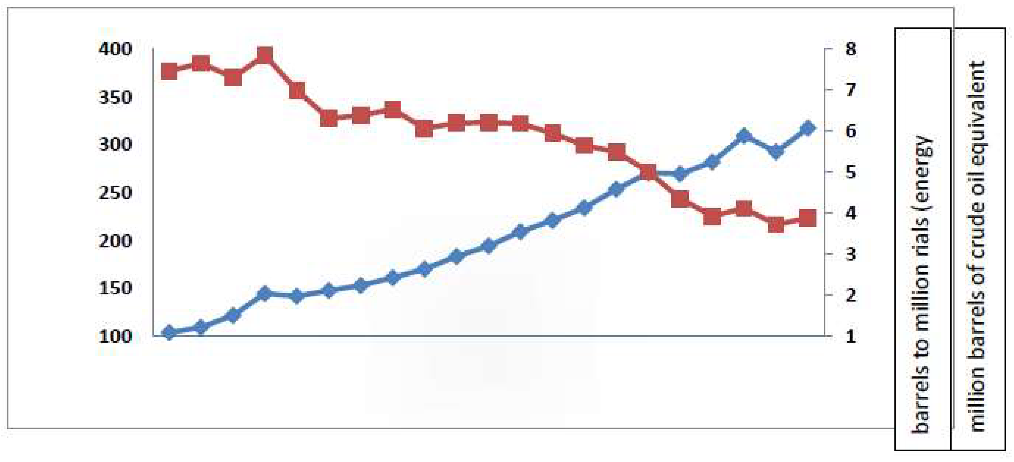
Before estimating the model, a detailed examination of the behavior of the variables used was conducted. This included analyzing the energy intensity of the transportation sector, the number of cars, and the clean and renewable energy production from 1991 to 2011. As per the data provided, energy consumption in the transportation sector stood at 104 million barrels of crude oil equivalent in 1991, increasing to 297.37 million barrels of crude oil equivalent in 2011, representing an average annual growth rate of 5.16%. By 2013, the transportation sector accounted for 24/23 percent of the total energy consumption in the country.

During this period, the growth of the added value of the transportation sector was 63.9% annually on average. Therefore, the energy intensity of the transportation sector, while the trend of energy consumption has been increasing, has decreased from 7.45 units in 1991 to 3.88 units in 2011 (Energy Balance Sheet 2013).

Figure 3. Energy consumption and intensity in the transportation sectorquote.

Figure 3. Energy consumption and intensity in the transportation sectorquote.

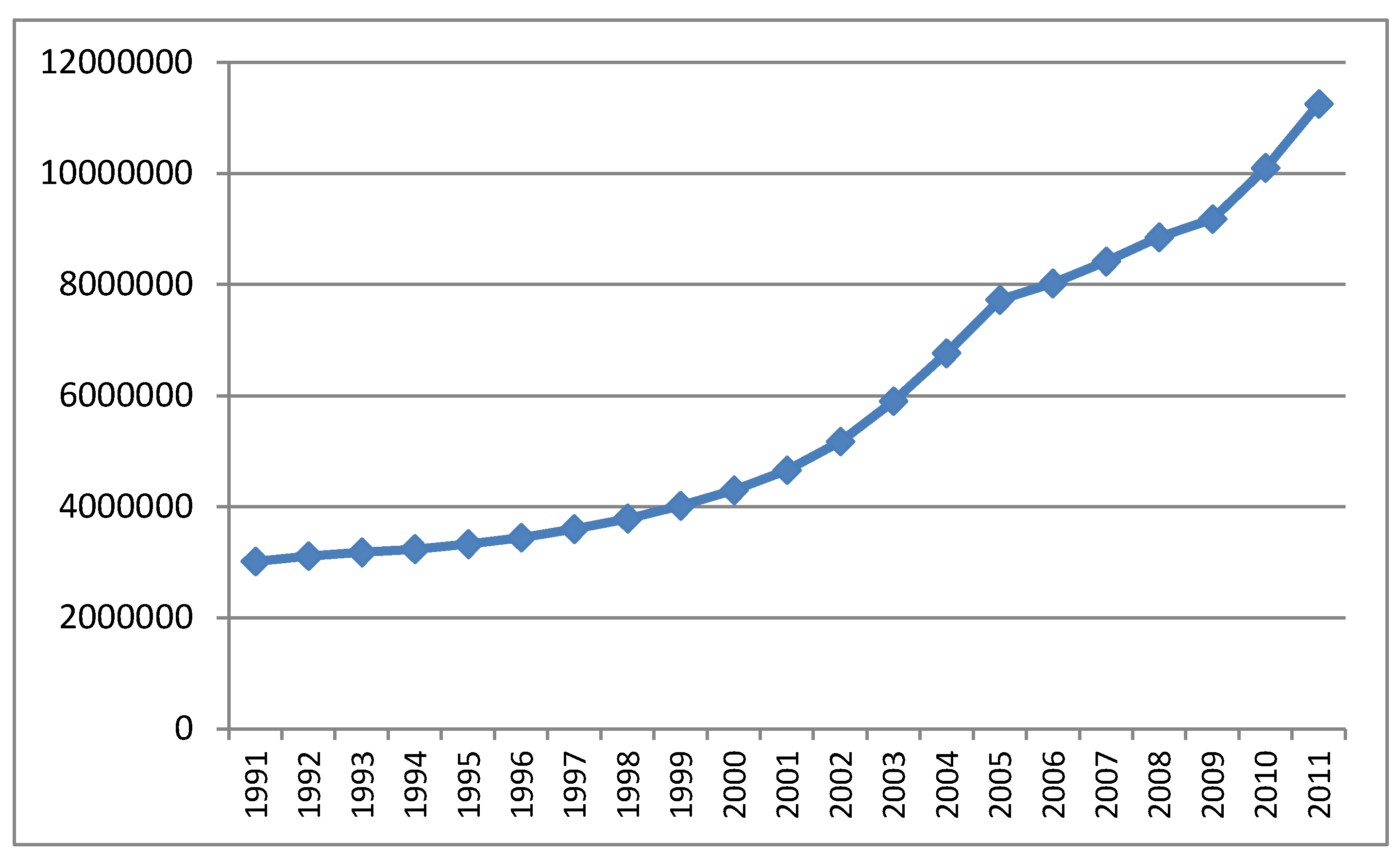
The examination of data concerning the generation of sustainable and environmentally-friendly energy between 1991 and 2011 reveals an average yearly increase of 5.66%, contributing to 1.7% of the nation’s total energy consumption. By 2011, clean and renewable energy production had reached 12 million barrels of crude oil equivalent. The Energy Balance Sheet for 2011 illustrates this growth. The chart provided depicts the progression of clean and renewable energy generation from 1991 to 2011.

Figure 4. The amount of production of clean and renewable energy (barrels equivalent to crude oil). Source: energy balance sheet.

Figure 4. The amount of production of clean and renewable energy (barrels equivalent to crude oil). Source: energy balance sheet.

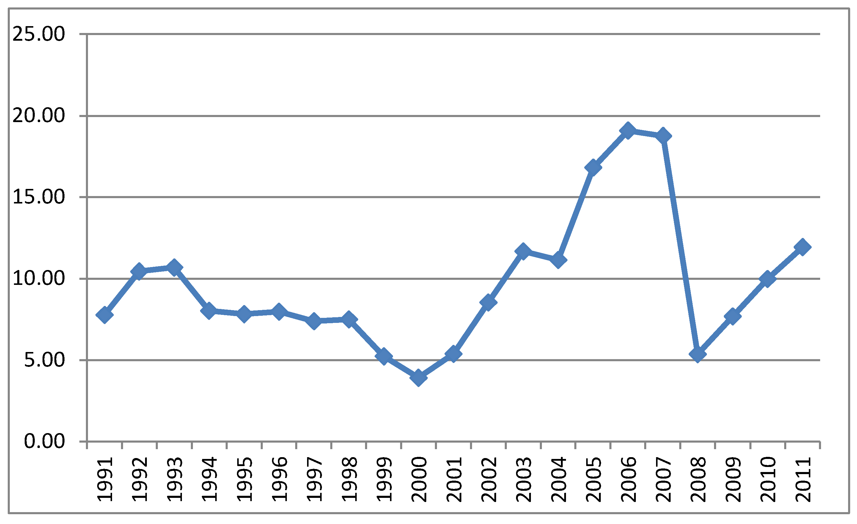
Figure 5. Number of cars during the period (1991-2011). Source: Ministry of Industry, Mining and Trade.

Figure 5. Number of cars during the period (1991-2011). Source: Ministry of Industry, Mining and Trade.

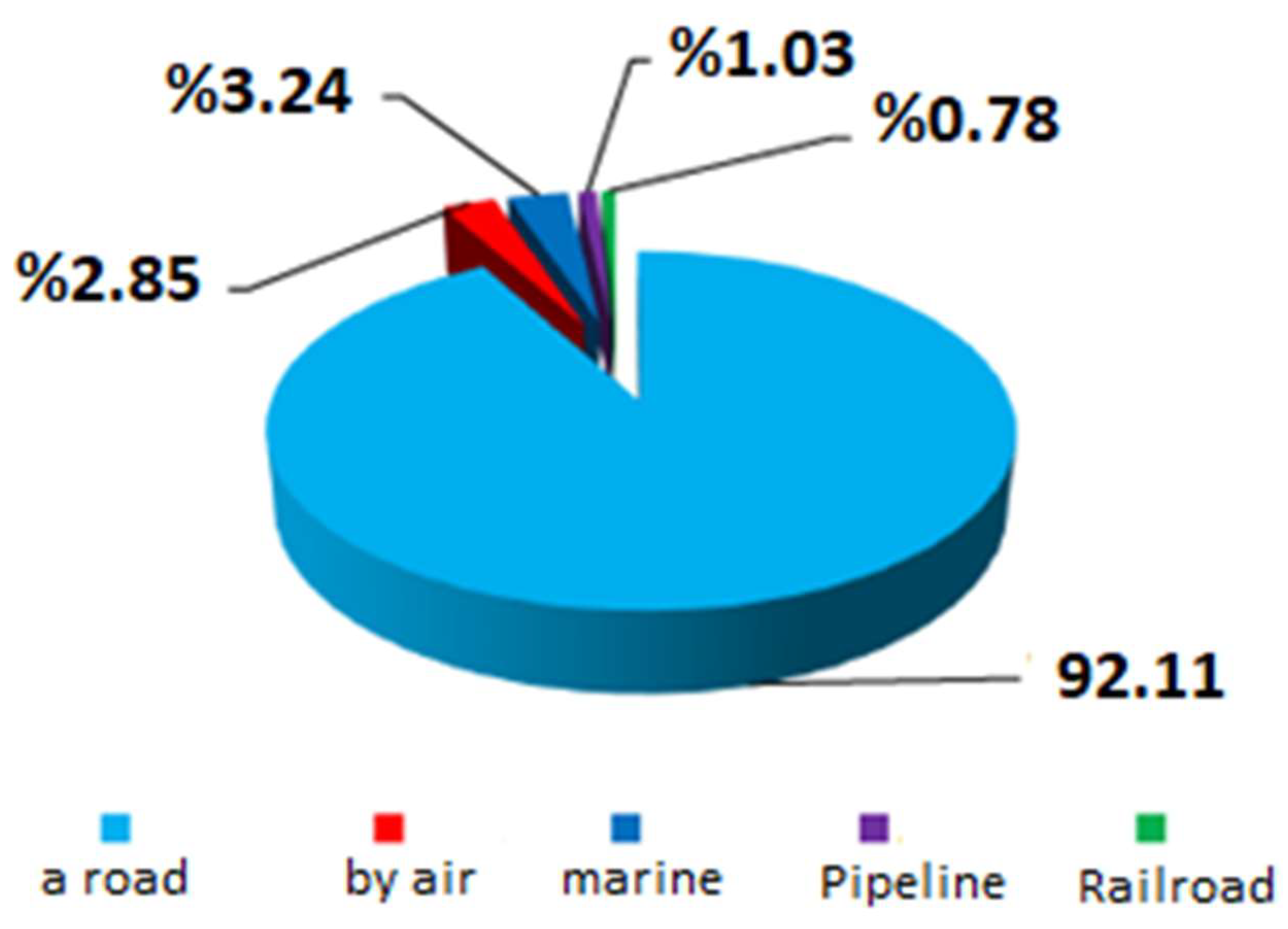
Examining the share of energy consumption in different modes of transportation in 2013 shows that road transportation had the largest share in energy consumption (92.11 percent) compared to other modes of transportation, and among them, transportation And rail transport, as the main competitor of road transport - especially in the movement of goods - has allocated less than one percent of energy consumption in the transport sector.

Figure 6. Share of energy consumption of the country’s transportation modes in 2011. Source: Energy balance sheet of the year 2013.

Figure 6. Share of energy consumption of the country’s transportation modes in 2011. Source: Energy balance sheet of the year 2013.

According to the presented statistics, the direction of transportation development should be focused on more energy efficiency in different modes.

4. Estimation of the Model and Analysis of the Results

The modern techniques of econometrics necessitate preliminary testing of the variables for reliability before estimating equation coefficients using time series data. Therefore, a consistent and dependable set of time series statistics for economic variables spanning 33 years was compiled to assess the reliability or lack thereof (Yaobin, 2009). The Generalized Dickey-Fuller test was applied to establish the collective order of each variable for this purpose. The reliability or instability of a time series holds significant implications for economic policies and estimation methods. One important implication of the reliability or instability of a time series in terms of economic policymaking is that a stable variable’s level cannot be permanently altered by economic policies, unlike an unstable variable whose level can be permanently changed by such policies. The significance of the reliability and collective order of time series variables becomes crucial when estimating equation coefficients, as variables sharing a common root can establish a long-term relationship economically (Abbasnejad, et al. 2014).

In the second step, after ensuring the collective order of the variables in each equation, the coefficients of the specified equations have been estimated. Since when the statistical sample size is small, the use of the ordinary least squares (OLS) estimation method will not provide a skewed estimate due to not taking into account the short-term dynamic reactions between the variables (Eskandari, et al. 2022), the model used In this article, the self-explanatory model is ARDL with extended intervals, which must be estimated first by using the OLS method for all possible combinations based on different intervals of the variables. The maximum number of intervals of variables is determined according to the number of observations.

In the second step, it is possible to select one of the estimated regressions based on the three rules of Akaik, Schwartz-Bazin, and Hanan-Coin. In the third step, the coefficients related to the long-term model are presented based on the selected ARDL model. In this model, in addition to long-term relationships, short-term error correction model (ECM) is also presented, which shows the speed of adjustment towards long-term balance. In fact, this method was chosen because (Behboodhi, et al. 2009):

• The ARDL method can be used regardless of whether the model variables are I(0) or I(1).
• By performing this method, economic analyzes can be performed in two short-term and long-term periods.
• The use of this method in small samples also has high efficiency due to the consideration of short-term dynamics between variables (Tashkini, 2015).

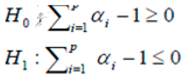
Before discussing the long-term equilibrium relationships, it is necessary to perform the unit root test of the null hypothesis of non-existence of convergence; because it is necessary that the dynamic model estimated in the ARDL method tends to long-term equilibrium, the sum of the coefficients of the dependent variable is less than one (Chung, et al. 2013).

The amount of t statistic needed to perform the above test is calculated as follows:

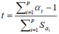
Upon comparing the t statistic and the critical value provided by Banerji, Dolado, and Master at varying confidence levels, it can be inferred that rejecting the H0 hypothesis implies the presence of a long-term equilibrium relationship among the variables in the model; otherwise, there is no such relationship. Acknowledging this long-term equilibrium allows for short-term estimation and consideration. The presence of convergence among a group of economic variables offers a statistical foundation for utilizing error correction models. These models are advantageous as they link the short-term fluctuations of variables to their long-term values. To adjust the error correction model, incorporating error terms associated with long-term convergence regression at a time lag as an explanatory variable alongside the first-order difference of other model variables is sufficient, followed by estimating the coefficients using the ordinary least squares method. Taking into account the estimation through the ARDL method entails including three categories of dynamic model equations, long-term equilibrium equations, and error correction models (ECM). All these procedures are carried out using Microfit 4 software, which will be elaborated on later in the discussion.

1.4. Unit Root Test

Before performing the cointegration test, the variables used in the model should be tested in terms of significance and hypothesis.

The presence of a single root in them should be investigated. This test was invented by Dickey and Fuller (1979 and 1981). The hypothesis of the unit root test is based on the generalized Dickey-Fuller (ADF) test as Equation (1).

$$\Delta X_t=\left(\rho -1\right)x_{t-1}+{\displaystyle \sum }_{j=1}^p{\lambda }_j\Delta x_{t-j}+{\epsilon }_t (1)$$

(1)

In Equation (1), xt is the variable at time t. ∆X_t is equal to xt-1-xt-2. And Ԑ_t has a mean of zero and a variance of σ^2. If the hypothesis H_0 that there is a random step process in the variable is confirmed, or in other words, ρ=1, then the variable is indeterminate.

This test can be performed in three modes without width from origin and trend, with width from origin and trend, and with width from origin and without trend. Given us is selected as the optimal model. The results of the unit root test for the level and the first order difference of the variables are given in Table 1.

Table 1. The results of the unit root test.

Stationary or unstationary variable	Dickie Fuller’s statistics	First order difference	Critical values at a significance level of 5%	Dickie Fuller’s statistics	Variable name
I(1)	-4.49	DLEIT	-2.95	-1.36	LEIT
I(1)	-4.33	DLEP	-2.95	-1.95	LEP
I(1)	-5.41	DLITVT	-2.95	-2.62	LITVT
I(1)	-3.98	DLKHOD	-2.95	-2.03	LKHOD
I(1)	-5.86	DLCE	-2.95	-2.79	LCE
I(1)	-3.7	DLPOP	-2.95	-2.89	LPOP

Source: research findings.

Table 1. The results of the unit root test.

Stationary or unstationary variable	Dickie Fuller’s statistics	First order difference	Critical values at a significance level of 5%	Dickie Fuller’s statistics	Variable name
I(1)	-4.49	DLEIT	-2.95	-1.36	LEIT
I(1)	-4.33	DLEP	-2.95	-1.95	LEP
I(1)	-5.41	DLITVT	-2.95	-2.62	LITVT
I(1)	-3.98	DLKHOD	-2.95	-2.03	LKHOD
I(1)	-5.86	DLCE	-2.95	-2.79	LCE
I(1)	-3.7	DLPOP	-2.95	-2.89	LPOP

Source: research findings.

It is important to mention that the maximum optimal score in the generalized Dickey-Fuller test is 9, and the Schwartz method was employed. The findings presented in Table 1 indicate that the τ statistic for the variables exceeds the critical values even at a 5% significance level, suggesting that the hypothesis of a unit root in the time series is not rejected. Essentially, the levels of variables utilized in the Namana model possess a unit root. However, upon differentiating the variables once in the model, all variables exhibit significance across all levels. Consequently, the τ statistic from the Dickey-Fuller test falls below the critical value at all levels, leading to the rejection of the unit root hypothesis and indicating that all variables in the convergent model are of first degree I(1).

The analysis conducted through the ARDL method involves the interpretation of three dynamic equations, long-term relationships, and error correction mechanisms. The Akaike, Schwartz-Bayesian, and Hannan-Quinn criteria, along with the adjusted coefficient of determination, can aid in determining the optimal lag length. In this research, the Schwartz-Bayesian criterion was utilized to preserve the degrees of freedom and avoid diminishing model accuracy.

2.4. Estimation of the Dynamic Coefficients of the Energy Intensity Equation of the Transportation Sector

$$LEIT=0.83*LEIT\left(-1\right)-0.2*LEP+0.22*LITVT-0.24*LKHOD-0.033*LCE+0.23*LPOP+0.15*D_{WAR}$$

That in the above relation

Dwar is a virtual variable whose quantity is equal to one for the years 59 to 66 and zero for the rest of the years.

Once the dynamic equation has been estimated, it is essential to conduct the Banerjee test to verify the presence of a sustainable relationship in the regression analysis. This test involves subtracting the coefficient of the dependent variable from one, dividing it by its standard deviation, and then comparing the resulting t-statistics (in absolute form) with the critical values from tables developed by Banerji, Dolado, and Mester. If the absolute value of the calculated test statistic exceeds the critical absolute value, it indicates a rejection of the null hypothesis of no co-integration between the variables in the model, thus confirming the existence of a long-term relationship.

$$\mathrm{T}\mathrm{B}={\displaystyle \frac{0.83-1}{0.09}}=-1.89$$

Therefore, it can be concluded that at the 75% confidence level, the null hypothesis of no cointegration between the pattern variables is rejected, and as a result, there is a long-term equilibrium relationship between the variables of the transport sector energy intensity pattern, which is as follows:

3.4. The Long-Term Balance Relationship of the Energy Intensity of the Transportation

Based on the t statistic, most variables are considered statistically significant. The variable coefficient for the relative price of energy indicates that a one-unit rise in energy prices leads to a decrease of 0.2 units in energy intensity in the short term and 1.2 units in the long term. The positive correlation between energy intensity and investment in the transportation industry suggests that increased investments have had a favorable and significant impact on energy intensity in transportation. Statistical analysis reveals that an average of 31,578.5 billion rials is annually invested in the machinery sector, equivalent to 71.9% of total transportation sector investments, while 9,949 billion rials are put into the construction sector. Data from the central bank suggests that due to the increasing energy consumption trend in the transportation industry and the extensive use of road transportation in the country, investments in the machinery sector may not have been as effective as needed, resulting in a lower increase in the transportation sector’s value added compared to energy consumption in the sector. Consequently, it can be inferred that the investments made have not been sufficient in reducing energy intensity in the transportation sector.

Table 2. Long-term equilibrium results of the energy intensity of the transportation sector.

[probability] test statistic	Estimated coefficient	explanatory variable
-1.94[.062]	-0.0417	Lep
1.83[.077]	1/39	Litvt
-2.75[.011]	-0.0196	LKHOD
-1.10[.27]	0	Lce
2.90[.007]	1/44	LPOP
1.17[.25]	0/96	DWAR

Table 2. Long-term equilibrium results of the energy intensity of the transportation sector.

[probability] test statistic	Estimated coefficient	explanatory variable
-1.94[.062]	-0.0417	Lep
1.83[.077]	1/39	Litvt
-2.75[.011]	-0.0196	LKHOD
-1.10[.27]	0	Lce
2.90[.007]	1/44	LPOP
1.17[.25]	0/96	DWAR

The coefficient obtained for the population variable indicates that as the population increases, energy consumption intensity in the transportation sector also increases. The results from the model estimation reveal that there was no significant correlation between energy intensity and clean fuels in the country. However, at a 70% significance level, an increase in the production of clean fuels led to a decrease in energy consumption intensity in the transportation sector.

Similarly, the coefficient for the number of cars variable suggests that during the review period, the number of cars negatively impacted energy intensity. This means that as the number of cars increased, energy consumption intensity in the transportation sector decreased. This can be attributed to two main factors. Firstly, the recent refurbishment of old cars has shortened the lifespan of the transportation fleet (both public and private cars), affecting energy consumption intensity. Secondly, global efforts to reduce car fuel consumption, despite the dominance of domestic car manufacturers, have had positive effects on both domestic and imported car sectors. The dual fuel utilization in cars has also played a role in this sector.

A correction-error model was then developed to explore how short-term imbalances in energy intensity in the transportation sector are adjusted towards long-term equilibrium. The ECM variable coefficient of -1 is crucial in error correction models. The results of the correction-error model estimation are presented in the table below:

Table 3. Results of the correction-error relationship for the energy intensity of the transport sector.

explanatory variable	Estimated coefficient	[probability] test statistic	Significant confidence level
Dlep	-0/20	-3.9055[.001]	0/95
Dlitvt	0/22	3.8916[.001]	0/95
dLKHOD	-0/24	-3.0499[.005]	0/95
Dlce	-0.33	-1.7796[.087]	0/90
dLPOP	0/23	2.9914[.006]	0/95
dDWAR	0/15	2.9803[.006]	0/95
ecm(-1)	-0/16	-1.6702[.107]	0/90

Source: Research findings.

Table 3. Results of the correction-error relationship for the energy intensity of the transport sector.

explanatory variable	Estimated coefficient	[probability] test statistic	Significant confidence level
Dlep	-0/20	-3.9055[.001]	0/95
Dlitvt	0/22	3.8916[.001]	0/95
dLKHOD	-0/24	-3.0499[.005]	0/95
Dlce	-0.33	-1.7796[.087]	0/90
dLPOP	0/23	2.9914[.006]	0/95
dDWAR	0/15	2.9803[.006]	0/95
ecm(-1)	-0/16	-1.6702[.107]	0/90

Source: Research findings.

Most of the variables in the equation are significant at the 95% level. The coefficient of correction-error term ECM(-1) is estimated as 0.16 and shows that in each period 16% of the imbalance in the energy consumption intensity of the transportation sector is adjusted and approaches its long-term trend.

5. Conclusions and Suggestions

In this study, the focus was on examining the factors influencing energy consumption in the transportation sector, using a dynamic econometric model to analyze the impact of these factors on energy intensity. Various techniques for analyzing time series data, such as unit root final test, cointegration analysis, and autoregression method with extended intervals (ARDL), were used to estimate model parameters based on data from 1979 to 2011. The results indicated that an increase in relative energy prices led to a decrease in energy consumption intensity, albeit small in the short term.

The research highlighted the challenges of reducing energy consumption intensity in the transportation sector, given the limited alternatives and low elasticity of energy demand, particularly in passenger and goods transport. The reliance on price policies alone was deemed ineffective, and the study suggested adopting complementary measures, such as taxing inefficient automobile manufacturers and imposing levies on environmental pollutants from cars, based on international experiences.

The analysis revealed that the number of cars negatively affected energy intensity, suggesting a decrease in energy consumption intensity as the number of cars increased. This trend reflected efforts in Iran to optimize fuel consumption by phasing out old and gas-guzzling vehicles in the transportation fleet. I’m sorry, but you have not provided any text to be paraphrased. Please provide the text that needs to be paraphrased so that I can assist you. Thank you.

The rise in population has a noticeable impact on the amount of energy used in the transportation industry, particularly due to the higher demand for passenger and freight services. To alleviate the strain on energy consumption caused by population growth in transportation, promoting the use of public transportation, improving public transportation networks in urban areas, minimizing unnecessary trips, utilizing information technology, and communication, can all help reduce travel within cities

References

- Abbasinejad, H.; Vafi Najjar, D. Investigation of energy efficiency and productivity in different economic sectors and estimation of input and price elasticity of energy in the industry and transportation sectors using the TSLS method. Economic Research 2014, 66, 137–113. (In Persion) [Google Scholar]
- Adom, P.K. Asymmetric impacts of the determinants of energy intensity in Nigeria. Energy Economics 2015, 49, 570–580. [Google Scholar] [CrossRef]
- Azizi, J. Evaluating the efficiency of Agricultural Bank branches using data coverage analysis model and determining a consolidated index (case study of Mazandaran province). Journal of Agricultural Economics 2014, 9, 63–76. (In Persion) [Google Scholar]
- Azizi, J.; Aref Eshghi, T. The Role of Information and Communication Technology (ICT) in Iranian Olive Industrial Cluster. Journal of Agricultural Science 2011, 3, 228–232. [Google Scholar] [CrossRef]
- Azizi, J.; Jabbari, A. Estimating Monetary Demand Using a Flexible Model of Almost Ideal Demand System (AIDS). Preprints 2024, 2024061596. [Google Scholar] [CrossRef]
- Behbodhi, Z.; et al. Analysis of energy intensity and the analysis of factors affecting it in Iran’s economy. Quarterly Journal of Energy Economics Studies 2009, 7, 105–130. (In Persian) [Google Scholar]
- Eskandari, S.; ZeraatKish, Y.; Moghaddasi, R.; Azizi, J. Determinant factors energy efficiency and emission of pollutants Co2 & So2 in Iran’s agricultural sector. Int. J. Environ. Sci. Technol. 2022, 19, 1717–1728. [Google Scholar] [CrossRef]
- Chung, W.; Zhou, G.; Yeung, I.M.H. A study of energy efficiency of transport sector in China from 2003. Applied Energy 2013, 112, 1066–1077. [Google Scholar] [CrossRef]
- Imam Vardi, A.; et al. (2012). Forecasting energy consumption in Iran using the dynamic system approach and econometrics, the first international conference on econometrics, methods and applications, Sanandaj.
- Jamshidi, M.M. (2008)”An Analysis of Residential Energy Intensity in Iran, A System Dynamics Approach”, Sharif University of Technology, Faculty of Computer Engineering.
- Jimenez, R.; Mercado, J. Energy intensity: A decomposition and counterfactual exercise for Latin American countries. Energy Economics 2014, 42, 161–171. [Google Scholar] [CrossRef]
- Khaksari, A.; Ardabili, P. Studying the Elasticity of Fuel Demand in Land Transportation in the Country. Economic Research Quarterly 2016, 6, 1–11. (In Persion) [Google Scholar]
- Minhaj, M.; et al. Forecasting the energy demand of the transportation sector using neural networks: a case study in Iran. Management Research in Iran 2018, 14, 203–220. (In Persion) [Google Scholar]
- Motfekrazad, M.A.; Gholami Heydariani, L. (2018). Investigating the mutual causality between energy consumption and economic growth in Iran’s transportation sector. 11th International Conference on Transportation and Traffic Engineering, Tehran. (In Persion).
- Mulder, P.; De Groot, H.L. Structural change and convergence of energy intensity across OECD countries, 1970–2005. Energy Economics 2012, 34, 1910–1921. [Google Scholar] [CrossRef]
- Pindyck, R.S. (1979), The Structure of World Energy Demand, MIT Press.
- Pongthanaisawan, J.; Sorapipatana, C. Relationship between level of economic development and motorcycle and car ownerships and their impacts and greenhouse gaz emission in Thailand. Renewable and Sustainable Energy Reviews 2010, 14, 2966–2975. [Google Scholar] [CrossRef]
- Razmi, S.A.; Azari, L. (2009). Informal transportation in Razavi Khorasan Province. Knowledge and Development Magazine, No. 20, first half of 2016. (In Persion).
- Salimifar MHaqnejad, A.; Rahimi, M. (2009). Investigating the effect of production factors on the intensity of energy consumption in Iran: an analysis based on the Cab-Douglas production function. Knowledge and Development Magazine, No. 34. 1-20. (In Persion).
- Seifipour, R.; Afrooz Amini, F. (2012). The effect of fuel price increase on rail cargo demand and its share in land transportation. Transportation Engineering / Third Year / Fourth Issue, 315-323.
- Sharifi, N. The position of transportation and its impact on other sectors of the country’s economy: a data-output analysis. Economic Growth and Development Researches 2013, 5, 207–237. [Google Scholar]
- Tahari Mehrjardi, M.; Maybadi, H.; Taghizadeh Mehrjardi, R. Modeling and forecasting of energy consumption in Iran’s transportation sector: application of artificial intelligence models. Program and Budget Quarterly 2011, 17, 29–47. (In Persion) [Google Scholar]
- Teshkini, A. (2015). Applied econometrics with the help of microfit. Dibagaran Cultural Institute Publications, Tehran.
- Yaobin, L. Exploring the relationship between urbanization and energy consumption in China using ARDL (autoregressive distributed lag) and FDM (factor decomposition model). Energy 2009, 34, 1846–1854. [Google Scholar]
- Zarei, N.; Azizi, J. Environmental impact assessment in Iran after its accession to the Shanghai cooperation organization: panel FMOLS analysis in two different income groups. Int. J. Environ. Sci. Technol. 2024. [CrossRef]
Disclaimer/Publisher’s Note: The statements, opinions and data contained in all publications are solely those of the individual author(s) and contributor(s) and not of MDPI and/or the editor(s). MDPI and/or the editor(s) disclaim responsibility for any injury to people or property resulting from any ideas, methods, instructions or products referred to in the content. |
© 2024 by the authors. Licensee MDPI, Basel, Switzerland. This article is an open access article distributed under the terms and conditions of the Creative Commons Attribution (CC BY) license (http://creativecommons.org/licenses/by/4.0/).
Copyright: This open access article is published under a Creative Commons CC BY 4.0 license, which permit the free download, distribution, and reuse, provided that the author and preprint are cited in any reuse.