
Submitted:
08 October 2024
Posted:
08 October 2024
You are already at the latest version
Abstract
Complexity is a crucial metric for evaluating urban intersection scenarios. However, existing complexity evaluations are often derived indirectly from the driving risk of autonomous vehicles, leading to subjective and incomplete evaluations. Therefore, this study undertakes a comprehensive evaluation of intersection scenarios from a systems perspective by quantifying the number of vehicles and the characteristics of vehicle interactions within the intersection.Specifically, we propose an objective framework for assessing complexity. In this framework, the number of vehicles serves as the foundation for assessment, while three interaction characteristics—interaction density, interaction disorder, and interaction risk—are modeled as scaling factors of complexity. In particular, by combining logistic and hyperbolic tangent functions, we accurately capture the nonlinear effects of vehicle numbers and interaction characteristics on complexity.The experimental results demonstrate that the evaluation outcomes of the proposed method are highly correlated with the risk and efficiency performance of autonomous vehicles at intersections, thereby validating the method. Additionally, this method is utilized to guide the generation of highly complex urban intersection scenarios, achieving double the generation efficiency compared to the random sampling method.
Keywords:
Autonomous driving tests
; urban intersections
; scenario complexity evaluation
; interaction density
; interaction disorder
; interaction risk
1. Introduction
Urban autonomous driving mobility services are widely regarded as one of the first major commercial applications of autonomous driving technology [1,2]. Although significant progress has been made in this field, substantial challenges remain for its large-scale deployment, particularly in processing complex city intersections, which have become a critical bottleneck [3]. First, the dense and chaotic driving environment at urban complex intersections significantly increases the perception, decision-making, and control challenges for autonomous driving systems [4,5], posing major obstacles to their safe operation. Second, considering the critical traffic hub role of urban complex intersections, the driving efficiency of autonomous systems in these scenarios must adhere to higher standards [6,7]. Therefore, sufficient testing of complex urban intersection scenarios is essential.
Enclosed-area testing, real-world testing, and simulation testing are the three principal methods currently employed for testing autonomous driving systems [8,9,10]. Among these, simulation testing has become the mainstream approach due to its safety and efficiency [11,12,13]. However, to ensure simulation serves as an effective testing tool, it is crucial to generate challenging and highly complex scenarios. Consequently, complexity, as a key evaluation index in scenario generation, has become the focus of current research.
However, current research primarily relies on the risk of an autonomous vehicle traveling through an intersection to indirectly assess complexity, typically based on the temporal and spatial proximity of vehicles. To describe the nonlinear relationship between risk and changes in temporal and spatial proximity, advanced models such as the information entropy model [14], the gravitational model [15,16], and field theory [17,18] have been introduced. For example, Zhou et al [18] treat dynamic traffic vehicles as charged particles and use the combination and superposition of potential fields to describe scene complexity. Similarly, Dong et al [19] evaluate the dynamic impact by assessing the gravitational influence of the lead vehicle on other vehicles. Some studies evaluate scenario complexity by measuring the maneuvering space available to the ego vehicle [20]. However, this indirect evaluation method has two major limitations: First, the method’s reliance on the performance of the ego vehicle compromises the objectivity of the results and reduces its versatility. Second, it overlooks the comprehensive interactions among all vehicles at the intersection, leading to an incomplete evaluation.
To address the above issues, this study developed an objective complexity evaluation framework. In this framework, the number of vehicles serves as the basic calculation unit, and the global interaction characteristics are quantified using three indicators: interaction density, interaction disorder, and interaction risk. Specifically: 1) The count of vehicles within the intersection area per unit time is measured, and a logistic function is employed to describe the non-linear impact of this number on complexity. 2) The interaction density is is defined as the ratio of the actual number of interactions at the intersection to the theoretical maximum possible interaction. 3) Interaction disorder is determined by comparing the actual disordered state with the number of changes in driving direction under ideal conditions. 4) The Interaction risk is calculated by the average collision probability among all interaction pairs. The amplification effect of these three features on complexity is modeled using the hyperbolic tangent function.
In the experimental part, we validated the effectiveness of the method by analyzing the correlation between scenario complexity and the performance of the autonomous driving system. The results of both the correlation and regression analyses demonstrate that the complexity evaluation from this method is highly correlated with the driving risk and efficiency assessments of autonomous driving at intersections. Additionally, this method has been successfully implemented on the Apollo autonomous driving platform to guide the generation of high-complexity test scenarios. Compared to the traditional random sampling method, it has doubled the efficiency of generating high-complexity scenarios, demonstrating its practical value in engineering applications.
The paper is organized as follows: Section 2 introduces the method for evaluating the complexity of urban intersection scenarios; Section 3 verifies the method’s effectiveness; Section 4 demonstrates its value for engineering applications; and finally, Section 5 summarizes the research conclusions and discusses future research directions.
2. Methods
The quantification of complexity typically encompasses three dimensions: the number of system elements, the diversity of these elements, and the relationships between them [21]. Diversity generally refers to the variety of element types within a system. In this study, we focus exclusively on a single type of traffic participant—vehicles. Consequently, we quantify the complexity of urban intersection scenarios based solely on the dimensions of quantity and relationships. The relationships between vehicles are further quantified using three key indicators: interaction density, interaction disorder, and interaction risk.
Referring to the complexity evaluation framework detailed in reference [22], the number of vehicles is considered the foundational characteristic of complexity, with the three interaction characteristics serving as scaling factors. Accordingly, the quantitative model of complexity can be expressed as follows:
where C represents the complexity of the urban intersection scenario, N is the number of vehicles in the scenario, and , and are the interaction density index, interaction disorder index, and interaction risk index, respectively. The function describes the relationship between the number of vehicles and the complexity, while , and represent the scaling relationships between the interaction density, interaction disorder, and interaction risk indices and the complexity, respectively.
2.1. Relationship Between the Number of Vehicles and Complexity
The number of vehicles serves as the foundation for determining the complexity of an urban intersection scenario. A higher number of vehicles typically indicates a potentially more complex interaction scenario. However, due to the sequential driving characteristics of intersections, not all vehicles contribute equally to the complexity. As illustrated in Figure 1, vehicles at the back of the queue must wait outside the intersection until the vehicles in front depart and vacate space before they can enter. Consequently, the primary contributors to the complexity of the scene are the vehicles within the intersection. Additionally, to account for the dynamic nature of the scene, we calculate the average number of vehicles in the intersection per unit time as the final count of vehicles present, as follows:
where represents the total number of vehicles in the intersection area at time t
The relationship between the number of vehicles and the complexity of the intersection is nonlinear. When there are few vehicles, the impact on complexity is minimal. As the number of vehicles reaches a moderate level, complexity increases sharply. However, when the number of vehicles becomes too high, the impact on complexity gradually diminishes. As shown in Figure 2, this phenomenon is analogous to population growth in biology, which is characterized by an S-shaped curve. Therefore, the logistic function is used in this study to describe the relationship between the number of vehicles in the scenario and complexity, as follows:
where is the growth rate parameter of the logistic function, which can be adjusted according to the road structure and geometric dimensions of different intersections. It is important to maintain a consistent value for road structures with the same dimensions to ensure the model’s evaluation results remain consistent across similar scenarios.
In addition, since the value range of the variable is , we need to map it to the input range of the logistic function using a linear transformation. The values of and are determined by solving the logistic function such that and , which represent the limit values of the function approaching 0 and 1 , respectively.
2.2. Relationship Between Interaction Density and Complexity
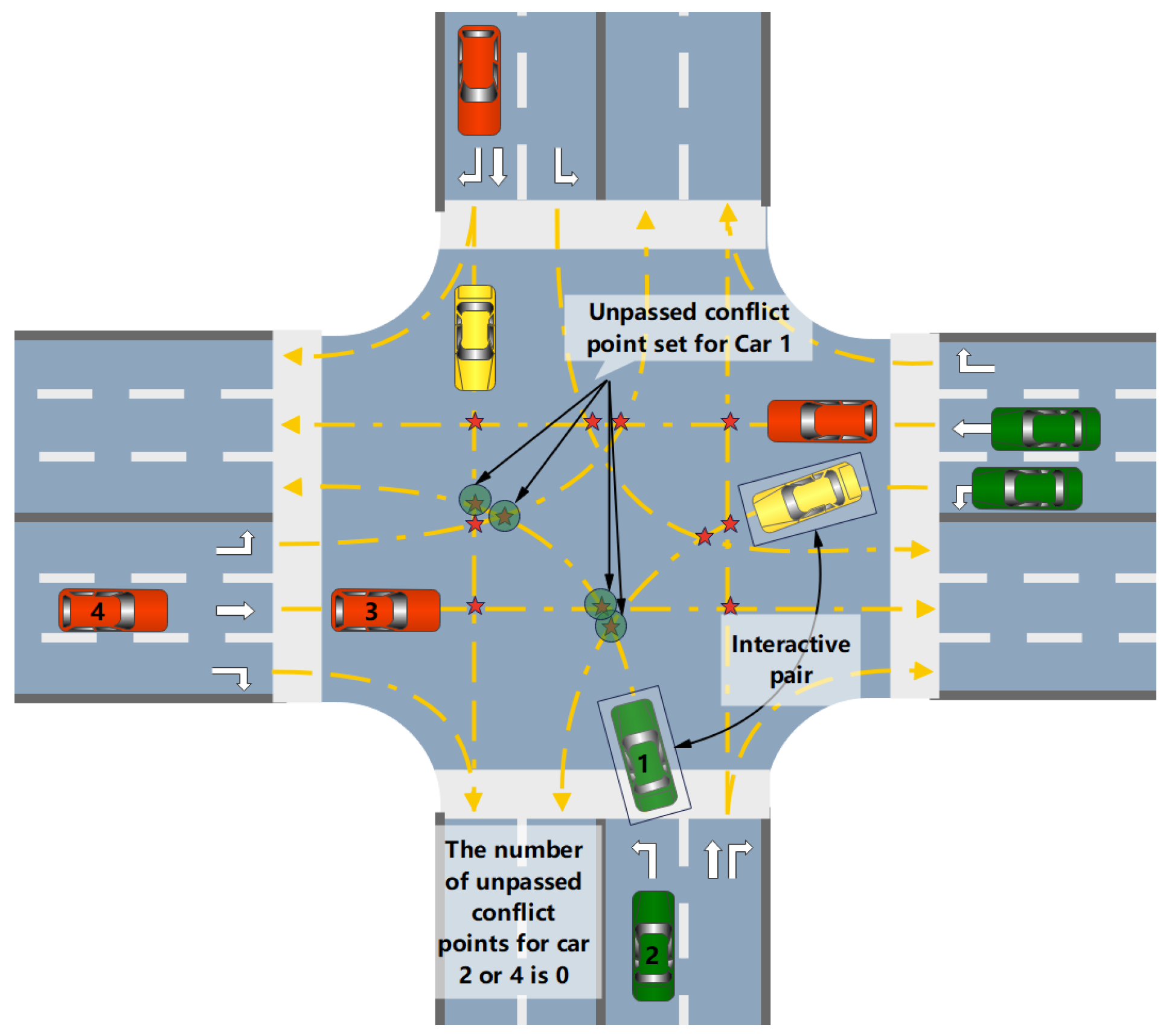
The interactions between vehicles in an urban intersection primarily occur at conflict points. With the same number of vehicles, a higher interaction density within the intersection results in greater scenario complexity. Interaction density is defined as the ratio of the actual number of interaction pairs among all vehicles in the intersection to the theoretical maximum number of interaction pairs within a unit of time. As shown in Figure 2, the two vehicles closest to a conflict point form a conflict interaction pair. If a vehicle is about to pass through a conflict point and there are no other vehicles between it and the conflict point, the conflict point is considered to be occupied. A vehicle can occupy multiple conflict points along its path that are not currently being passed through. The calculation formula is as follows:
where T is the total simulation step length, represents the actual number of interactions at the intersection at time t, and represents the theoretical maximum number of interactions at the intersection at time t. The calculation of the assumes that there is a interacting object at every unpassed conflict point ahead of each vehicle.
Figure 3.
Schematic diagram for calculating the number of vehicle interactions.
When the interaction density is equal to 0, it indicates that there is no conflict interaction between any vehicles in the scene, meaning that the movement of all vehicles does not cause potential interference. In this case, the complexity of the scene should be 0, meaning the amplification factor of the interaction density is also 0. As the interaction density increases, the number of conflicting interactions between vehicles rises, leading to a greater amplification effect of interaction density on complexity. This change can be effectively described by the hyperbolic tangent function (tanh). Therefore, the scaling relationship between interaction density and complexity can be expressed as follows:
where is an adjustable hyperparameter that influences the variation characteristics of the function. The appropriate value of can be determined experimentally or empirically, depending on the data distribution and the specific requirements of the application. A larger value makes the function more sensitive near the zero point, while a smaller value results in a smoother function. Figure 4 visually illustrates the effect of the value on the shape of the function.
2.3. Relationship Between Interaction Disorder and Complexity
At un-signalized intersections, vehicles often do not adhere strictly to road rules in an orderly manner. Instead, the order of travel is typically determined by a free-for-all approach, which introduces a distinct element of chaos and disorder. The more disorderly the interactions between vehicles, the greater the complexity of the scenario. As shown in Figure 5, in an ideal orderly scenario, the driving direction at each conflict point changes only once. Conversely, in disorderly situations, vehicles may not fully comply with established rules, leading to both sides of the conflict attempting to pass alternately. This behavior results in multiple changes in the driving direction at the conflict point. The greater the number of changes, the higher the disorder of the scenario. Based on the preceding analysis, this study defines interactive disorder as the ratio of the number of changes in driving direction observed in the actual disordered state to those in the ideal state. The calculation is performed as follows:
where represents the number of changes in driving direction under idealized ordered conditions, and represents the number of changes in driving direction under actual conditions.
Due to the limited capacity of the intersection area, vehicles often need to enter in sequence, which causes the chaotic characteristics to average out over time. This phenomenon can result in an overestimation of the interaction disorder index. To correct for this, we introduce a time-averaging factor:
where N is the total number of vehicles in the scenario.
when , it indicates that all vehicles enter and leave the intersection simultaneously, making the calculation result most accurate, with no further correction needed. If , it means that vehicles enter and leave the intersection gradually. In this case, using to reduce the value of the can help minimize the deviation in the calculation result. The final corrected disorder index is:
The scaling relationship between the complexity of interaction disorder and interaction density is similar. Accordingly, using the hyperbolic tangent function, the scaling relationship between the complexity of interaction disorder and overall complexity can be expressed as follows.
where is a hyperparameter.
2.3.1. Relationship Between Interaction Risk and Complexity
The high density of interactions and the chaotic nature of urban intersections significantly increase the probability of collisions between vehicles, leading to a high-risk interaction environment. In this study, interaction risk is defined as the average collision likelihood of all interaction pairs per unit time, calculated as follows:
where T is the total simulation step length, ’pair’ represents the combination of the serial numbers of all interaction pairs, is the total number of interaction pairs, and is the collision probability of vehicle i and vehicle j at the collision point in the interaction pair.
The collision likelihood of each vehicle pair is evaluated based on their spatial and temporal proximity to the collision point. The sum of the times at which each vehicle pair reaches the collision point, along with the time difference between them, serve as two key quantitative indicators that measure their proximity. The smaller the sum of times at which each vehicle pair reaches the point of conflict, the closer they are to converging at that location, thereby increasing the risk of collision. Similarly, a smaller time difference between the vehicles as they approach the conflict point indicates a higher likelihood that they will meet there, thus elevating the associated risk. Therefore, we combine the product of these two indicators and use a Gaussian function to model this negative correlation, constructing the collision risk for each vehicle pair, which is expressed as:
where and are the distances from the collision point to vehicles i and and are the speeds of vehicles i and j, and c is the standard deviation of the Gaussian function. By further exponentiation, we can simplify the expression as follows:
Similarly, using the hyperbolic tangent function, the scaling relationship between interaction risk and complexity can be expressed as follows:
where is a hyperparameter.
3. Validation and Results
This section aims to verify the effectiveness of the evaluation method. First, we visually demonstrate the method’s effectiveness through three specific evaluation cases. Second, we further validate the method by correlating the complexity evaluation results of the scenarios with the performance evaluation results of autonomous driving.
Section 3.1 introduces the simulation platform used in this experiment. Section 3.2 presents three specific evaluation cases. Section 3.3 outlines the design process of the method verification experiment and presents the experimental results.
3.1. Simulation Platform
As shown in Figure 6, a PanoSim-Apollo co-simulation framework was established for this study. In this framework, PanoSim serves as the scenario simulation platform, while the advanced autonomous driving system Apollo is the test object. PanoSim (version 5.0) and Apollo (version 7.0) run on different operating systems, Windows 11 and Ubuntu 18.04, respectively, with the two systems communicating via the UDP protocol. During the simulation, PanoSim sends scenario data to Apollo’s decision-making and planning module via Ethernet. After processing the data, Apollo returns the calculated vehicle control commands (throttle, steering, and braking) to PanoSim’s high-precision vehicle dynamics module to update the simulation state.
As shown in Figure 7, PanoSim is a high-performance scenario simulator developed by our team for research on autonomous vehicles. This platform integrates an accurate vehicle dynamics model, a highly realistic driving and traffic environment simulation, versatile onboard sensor models, and a wide range of test scenarios. It provides comprehensive testing capabilities, making it an ideal tool for addressing various autonomous driving testing needs.
3.2. Case Studies
This section visually demonstrates the evaluation effect of the method by comparing three urban intersection scenarios, which vary significantly in complexity. These scenarios were generated using the urban complex intersection scenario simulation model built into the PanoSim simulation software.
Figure 8(a–c) display key frame screenshots for three respective cases. Figure 8(a) illustrates case 1, where fewer vehicles at the intersection lead to simpler interaction characteristics. Conversely, Figure 8(b,c) show cases 2 and 3, where increased vehicle density leads to more complex interactions. The complexity evaluation results of 0.10, 0.47, and 0.69 for each case respectively, demonstrate that this evaluation method accurately reflects reality and can finely differentiate between scenarios of varying complexity.
3.3. Method Validation
This section verifies the method’s effectiveness by analyzing the correlation between the scenario’s complexity index and the autonomous driving system’s performance index. Specifically, a stronger correlation indicates a more reliable method.
3.3.1. Verify Data Collection
We generated a series of urban intersection scenarios of varying complexity using the built-in scenario models of the PanoSim platform. Based on these scenarios, we tested the Apollo autonomous driving system for unprotected left turns. Each set of experimental data collected detailed records of three key variables: scenario complexity, autonomous driving risk, and driving efficiency.
The specific simulation settings are illustrated in Figure 9. In this scenario, the Apollo vehicle executing a left turn encounters traffic from the north, east, and west, covering six lanes. The planned path of the Apollo vehicle is marked by a red curve. The maximum number of vehicles allowed in each lane is set to two. During the initialization phase of the simulation, these vehicles are randomly positioned within their respective lanes, with the distances between vehicles and their initial speeds randomly determined within the ranges of [3,10] meters and [0,5] meters per second, respectively. The simulation continues until all vehicles have safely exited the intersection or until the maximum simulation time of 60 seconds is reached.
The performance metrics for autonomous driving include:
(1) Risk metric: The average risk of conflict for self-driving vehicles is calculated using the formula below:
where represents the conflict risk between the ego vehicle and the conflicting vehicle j at time t. Here, M denotes the total number of conflicting vehicles for the ego vehicle, and T represents the total number of simulation steps.
(2) Efficiency metric: The average speed of an autonomous vehicle passing through an intersection is calculated using the formula below:.
where, denotes the speed of the ego vehicle at time t.
In this study, a total of simulation experiments were conducted. During the data processing phase, we eliminated abnormal data resulting from timeouts and unreasonable collisions. After this screening process, the total number of valid experimental datasets was . Table 1 shows the statistical results of the data set.
3.3.2. Verification Process
In this section, we initially employ the Pearson correlation coefficient to analyze the linear correlations among scenario complexity, driving risk, and efficiency. The higher the Pearson correlation coefficient, the stronger the linear relationship between the scenario’s complexity and the performance indicators. This indicates a higher effectiveness of the evaluation method. The specific formula for this calculation is as follows:
where and are the observed values of the variables, and x and y represent the mean values of these variables. A value of r close to +1 or -1 indicates a strong positive or negative linear relationship between the variables. The correlations between scenario complexity and both risk and efficiency are assessed independently.
Second, we employed linear regression analysis to thoroughly explore the specific impact of scenario complexity on driving risk and efficiency. The following linear regression model was employed:
where, y represents the measured value of driving risk or efficiency, while x denotes the complexity of the scenario. The coefficients and represent the intercept and slope, respectively, and signifies the error term. Additionally, a goodness-of-fit test is employed to assess the accuracy of the model’s predictions and the explanatory power of the explanatory variables. The specific calculation formula is provided below:
where , y represents the measured value of risk or efficiency, denotes the mean value of risk or efficiency, and indicates the predicted value from the regression.
3.3.3. Verification Results
Table 2 presents the results of the correlation analysis between complexity and risk, as well as between complexity and efficiency. The correlation coefficient between complexity and risk is , indicating a strong positive correlation. Additionally, the significance p-value is , confirming that this correlation is statistically significant. Simultaneously, the correlation coefficient between complexity and efficiency is , indicating a strong negative correlation. The significance p-value of further confirms that this negative correlation is statistically significant. These results clearly demonstrate that as the scenario complexity increases, the risk associated with autonomous driving rises and efficiency declines. This indicates a high correlation between the outcomes of the scenario complexity assessment and the autonomous driving performance evaluation, thereby verifying the effectiveness of our evaluation method.
The regression analysis results presented in Table 3 confirm a significant positive correlation between scenario complexity and the risk of automated driving. The regression coefficient is , indicating that for every unit increase in complexity, the risk increases by units. The goodness-of-fit value, , suggests that the model accounts for of the variance in risk. The results of the regression analysis in Figure 10 further elucidate the reasons behind the low values observed. While the overall trend indicates that risk increases with rising complexity, there is a noticeable point at which complexity reaches a certain threshold and then abruptly decreases. This sudden change leads to more divergent results, consequently affecting the model’s goodness of fit. This phenomenon occurs when the system, confronted with complex scenarios, adopts a conservative strategy, which consequently leads to a low risk assessment. Figure 11 displays key frame snapshots from two distinct test cases. In Figure 11(a), under conditions of low complexity, Apollo adopts an aggressive strategy to secure a lane, demonstrating its capability to effectively manage simple vehicle interactions and enhance traffic efficiency through competitive maneuvers. Conversely, Figure 11(b) depicts a scenario where Apollo, facing high complexity, opts to hesitate, allowing other vehicles to pass before proceeding, thus prioritizing safety.
The regression analysis results presented in Table 4 further substantiate a significant negative correlation between scenario complexity and the efficiency of autonomous driving. The regression coefficient is , indicating that for every unit increase in complexity, efficiency is expected to decrease by units. The goodness of fit value of demonstrates that the complexity provides a robust explanation for variations in efficiency. Figure 12 illustrates the regression analysis results concerning the relationship between scenario complexity and autonomous driving efficiency. The graph clearly shows a significant decrease in efficiency as complexity increases. This trend is consistent with the statistical data from the regression analysis, further confirming the strong negative correlation between scenario complexity and autonomous driving efficiency.
In summary, the results from both the correlation and regression analyses demonstrate a high correlation between the complexity evaluation of this method and the outcomes of risk and efficiency assessments for autonomous driving at intersections. These findings confirm the effectiveness and reliability of this evaluation method.
4. Applications in Generating Highly Complex Scenarios
This section will demonstrate the application of this evaluation method to the generation of highly complex scenarios at urban intersections to verify its engineering value.
4.1. Optimized Generation Method for Highly Complex Scenarios
This study searches for high-complexity urban intersection scenarios based on genetic algorithms. As shown in Figure 13, the method first encodes the input scenario parameters, and then generates new scenarios through an evolutionary process of crossover, mutation, and selection. Fitness is calculated based on a complexity index, and once the complexity of a scenario exceeds a set threshold, it is stored in the scenario library. Unlike the goal of traditional optimization searches, which seeks the optimal solution, this study aims to generate as many solutions as possible that meet the conditions, so a complete replacement selection strategy is used. Under this strategy, the parent individuals will be completely replaced by their offspring. In each generation, the algorithm only evaluates the newly generated offspring and does not retain any parent individuals. In the genetic algorithm setup, the population size is set to 10, with a crossover rate of 0.8 and a mutation rate of 0.01. The algorithm is configured to run for a maximum of 10,000 iterations.
As depicted in Figure 14, the scenario parameters include initial lanes , initial positions , initial velocities , and driving characteristic parameters . Here, x represents the initial position of each vehicle in its lane, defined using Frenet coordinates along the lane centerline. The driving characteristics parameter p assumes the values 1,2 , and 3 , corresponding to conservative, normal, and aggressive driving behaviors, respectively. These characteristics are predefined by the scenario model embedded in PanoSim. In this experiment, the total number of vehicles, N, is set at 10.
As depicted in Figure 13, we have implemented a segment encoding strategy, taking into account that the initial position, initial speed, and driving characteristic parameters represent different types of variables. This strategy organizes the chromosome into several distinct segments, with each segment containing genes of a single type. Specifically, each chromosome is divided into four segments: the initial lane sequence, the initial coordinate sequence, the initial speed sequence, and the driving characteristic sequence. Each segment contains genes that correspond to the respective parameter values for each vehicle, arranged in the appropriate order. Consequently, the total length of each chromosome is . In addition, given the strict requirements for vehicle position matching, and to prevent unreasonable vehicle configurations resulting from large-scale modifications, we employed a small-scale single-point crossover strategy. This strategy allows for minor adjustments based on the parent gene, ensuring that changes remain controlled and reasonable.
4.2. Generate Results
This experiment sets the high complexity threshold at 0.25. Figure 15 illustrates a comparison between the proposed method and the random sampling method concerning the generation rate of highly complex scenarios. The left y-axis displays the cumulative number of high-complexity scenarios generated, whereas the right y-axis shows the ratio of the generation rates between the proposed method and the random sampling method. The figure clearly demonstrates that the generation rate of the proposed method is significantly superior to that of the random sampling method. After 6,000 iterations, the generation rate of the proposed method stabilizes at approximately twice that of the random sampling method. In conclusion, the proposed method substantially improves test efficiency by accelerating the generation of high-complexity scenarios, thus proving its substantial value for engineering applications.
5. Conclusions
This study introduces a novel method for evaluating the complexity of urban intersection scenarios. This approach quantifies both the number of vehicles and the global characteristics of vehicle interactions at intersections, including interaction density, interaction disorder, and interaction risk, to provide a more objective and comprehensive evaluation. We experimentally validated the significant correlation between the proposed method and the risk and efficiency performance of autonomous driving systems at intersections through correlation analysis. In addition, the method is used to guide the generation of high-complexity scenarios at urban intersections, which is twice as efficient as random sampling methods, thus confirming its value in engineering applications. However, current research has not explored how signal light phases and road structures contribute to complexity. We plan to further enhance and expand the model in our future research endeavors.
Author Contributions
Conceptualization, Wang Ying and Deng Weiwen; Funding acquisition, Wang Ying and Ding Juan; Methodology, Li Jiangkun and Zong Ruixue; Software, Zong Ruixue and Ding Juan; Validation, Li Jiangkun and Zong Ruixue; Writing – original draft, Li Jiangkun; Writing – review & editing, Zong Ruixue, Wang Ying and Deng Weiwen. All authors have read and agreed to the published version of the manuscript.
Funding
This research was jointly funded by the "Lingyan" R&D Program of Zhejiang Province under Grant 2023C01238, "Jianbing" R&D Program of Zhejiang Province under Grant 2023C01133 and Jilin Provinice Science and Technology Project under Grant 20200501012GX.
Institutional Review Board Statement
Not applicable.
Informed Consent Statement
Not applicable.
Data Availability Statement
The datasets used during the current study are available from the corresponding author on reasonable request. The data are not publicly available due to privacy.
Acknowledgments
We would like to express our gratitude to PanoSim for their support in facilitating our experiment.
Conflicts of Interest
The authors declare no conflict of interest.
References
- Dai, J.; Wang, X.C.; Ma, W.; Li, R. Future Transport Vision Propensity Segments: A Latent Class Analysis of Autonomous Taxi Market. Transportation Research Part A: Policy and Practice 2023, 173, 103699. [Google Scholar] [CrossRef]
- Mao, W.; Shepherd, S.; Harrison, G.; Xu, M. Autonomous Vehicle Market Development in Beijing: A System Dynamics Approach. Transportation Research Part A: Policy and Practice 2024, 179, 103889. [Google Scholar] [CrossRef]
- Li, J.; Deng, W.; Wang, Y.; Wang, J.; Ding, J. Modeling of Complex Traffic Interaction Under Uncontrolled Intersection Scenario. IEEE Transactions on Intelligent Vehicles, 2024; 1–12. [Google Scholar]
- sele, D.; Rahimi, R.; Cosgun, A.; Subramanian, K.; Fujimura, K. Navigating Occluded Intersections with Autonomous Vehicles Using Deep Reinforcement Learning. 2018 IEEE International Conference on Robotics and Automation (ICRA), 2018, pp. 2034–2039.
- Tian, C.; Victor Chan, W.K.; Zhang, Y. Pedestrian Behavior at Intersections: A Literature Review of Models and Simulation Recommendations. 2020 Winter Simulation Conference (WSC), 2020, pp. 1194–1205.
- He, X.; Yang, L.; Lu, C.; Li, Z.; Gong, J. Adaptive Decision Making at the Intersection for Autonomous Vehicles Based on Skill Discovery. 2022 IEEE 25th International Conference on Intelligent Transportation Systems (ITSC), 2022, pp. 2842–2847.
- Yuan, T.; Zhao, X.; Liu, R.; Yu, Q.; Zhu, X.; Wang, S.; Meinke, K. Driving Intention Recognition and Speed Prediction at Complex Urban Intersections Considering Traffic Environment. IEEE Transactions on Intelligent Transportation Systems 2024, 25, 4470–4488. [Google Scholar] [CrossRef]
- Castellano, E.; Cetinkaya, A.; Arcaini, P. Analysis of Road Representations in Search-Based Testing of Autonomous Driving Systems. 2021 IEEE 21st International Conference on Software Quality, Reliability and Security (QRS), 2021, pp. 167–178.
- Karunakaran, D.; Berrio, J.S.; Worrall, S.; Nebot, E. Challenges Of Testing Highly Automated Vehicles: A Literature Review. 2022 IEEE International Conference on Recent Advances in Systems Science and Engineering (RASSE), 2022, pp. 1–8.
- Khan, F.; Falco, M.; Anwar, H.; Pfahl, D. Safety Testing of Automated Driving Systems: A Literature Review. IEEE Access 2023, 11, 120049–120072. [Google Scholar] [CrossRef]
- Feng, S.; Feng, Y.; Yu, C.; Zhang, Y.; Liu, H.X. Testing Scenario Library Generation for Connected and Automated Vehicles, Part I: Methodology. IEEE Transactions on Intelligent Transportation Systems 2021, 22, 1573–1582. [Google Scholar] [CrossRef]
- Feng, S.; Feng, Y.; Sun, H.; Bao, S.; Zhang, Y.; Liu, H.X. Testing Scenario Library Generation for Connected and Automated Vehicles, Part II: Case Studies. IEEE Transactions on Intelligent Transportation Systems 2021, 22, 5635–5647. [Google Scholar] [CrossRef]
- Zong, R.; Deng, W.; Bai, X.; Wang, Y.; Ding, J. Traffic Modeling Based on Data-Driven Method for Simulation Test of Autonomous Driving. IEEE Transactions on Intelligent Transportation Systems 2023, 24, 14076–14085. [Google Scholar] [CrossRef]
- Huang, P.; Ding, H.; Chen, H. An Entropy-Based Model for Quantifying Multi-Dimensional Traffic Scenario Complexity. IET Intelligent Transport Systems 2024, 18, 1289–1305. [Google Scholar] [CrossRef]
- Yang, S.; Gao, L.; Zhao, Y.; Li, X. Research on the Quantitative Evaluation of the Traffic Environment Complexity for Unmanned Vehicles in Urban Roads. IEEE Access 2021, 9, 23139–23152. [Google Scholar] [CrossRef]
- Dong, X.; Zhang, D.; Mu, Y.; Zhang, T.; Tang, K. Complexity of Driving Scenarios Based on Traffic Accident Data. International Journal of Automotive Technology 2024, 25, 23–36. [Google Scholar] [CrossRef]
- Cheng, Y.; Liu, Z.; Gao, L.; Zhao, Y.; Gao, T. Traffic Risk Environment Impact Analysis and Complexity Assessment of Autonomous Vehicles Based on the Potential Field Method. International Journal of Environmental Research and Public Health 2022, 19, 10337. [Google Scholar] [CrossRef] [PubMed]
- Zhou, J.; Wang, L.; Wang, X. Scalable Evaluation Methods for Autonomous Vehicles. Expert Systems with Applications 2024, 249, 123603. [Google Scholar] [CrossRef]
- Dong, X.; Zhang, D.; Mu, Y.; Zhang, T.; Tang, K. Complexity of Driving Scenarios Based on Traffic Accident Data. International Journal of Automotive Technology 2024, 25, 23–36. [Google Scholar] [CrossRef]
- Zhang, L.; Ma, Y.; Xing, X.; Xiong, L.; Chen, J. Research on the Complexity Quantification Method of Driving Scenarios Based on Information Entropy. 2021 IEEE International Intelligent Transportation Systems Conference (ITSC), 2021, pp. 3476–3481.
- Xing, J. Information Complexity in Air Traffic Control Displays. Human-Computer Interaction. HCI Applications and Services; Jacko, J.A., Ed.; Springer: Berlin, Heidelberg, 2007; pp. 797–806. [Google Scholar]
- Yu, R.; Zheng, Y.; Qu, X. Dynamic Driving Environment Complexity Quantification Method and Its Verification. Transportation Research Part C: Emerging Technologies 2021, 127, 103051. [Google Scholar] [CrossRef]
Figure 1.
Schematic diagram illustrating the division between the inner and outer areas of an urban intersection.
Figure 1.
Schematic diagram illustrating the division between the inner and outer areas of an urban intersection.
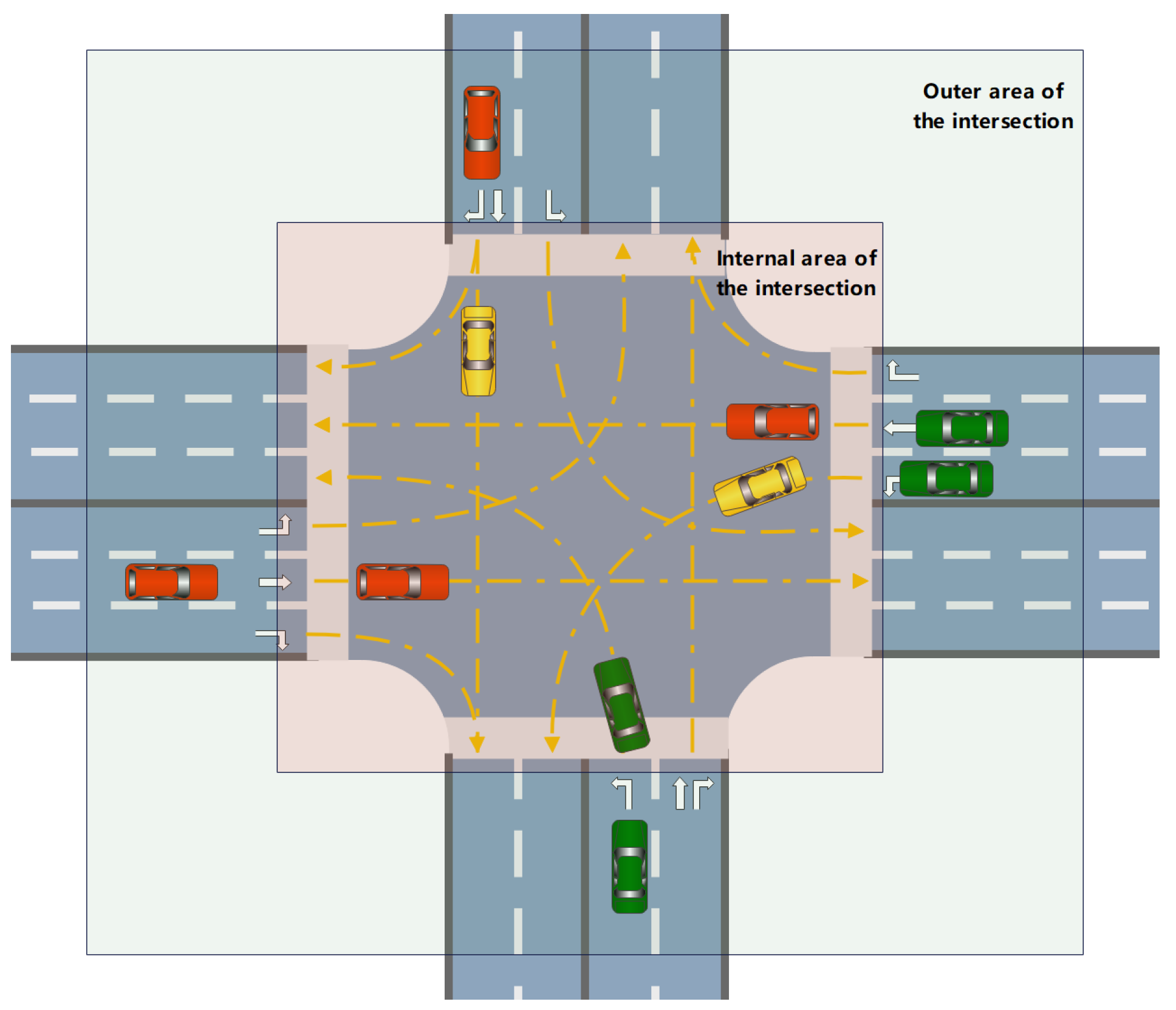
Figure 2.
The graph of the logistic function.
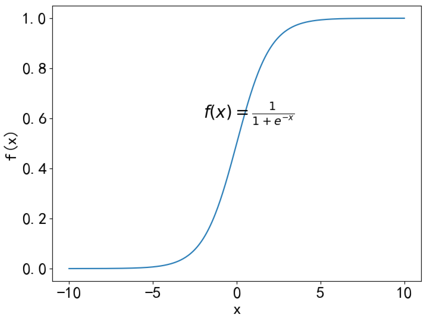
Figure 4.
The effect of different k values on the shape of the tanh function.
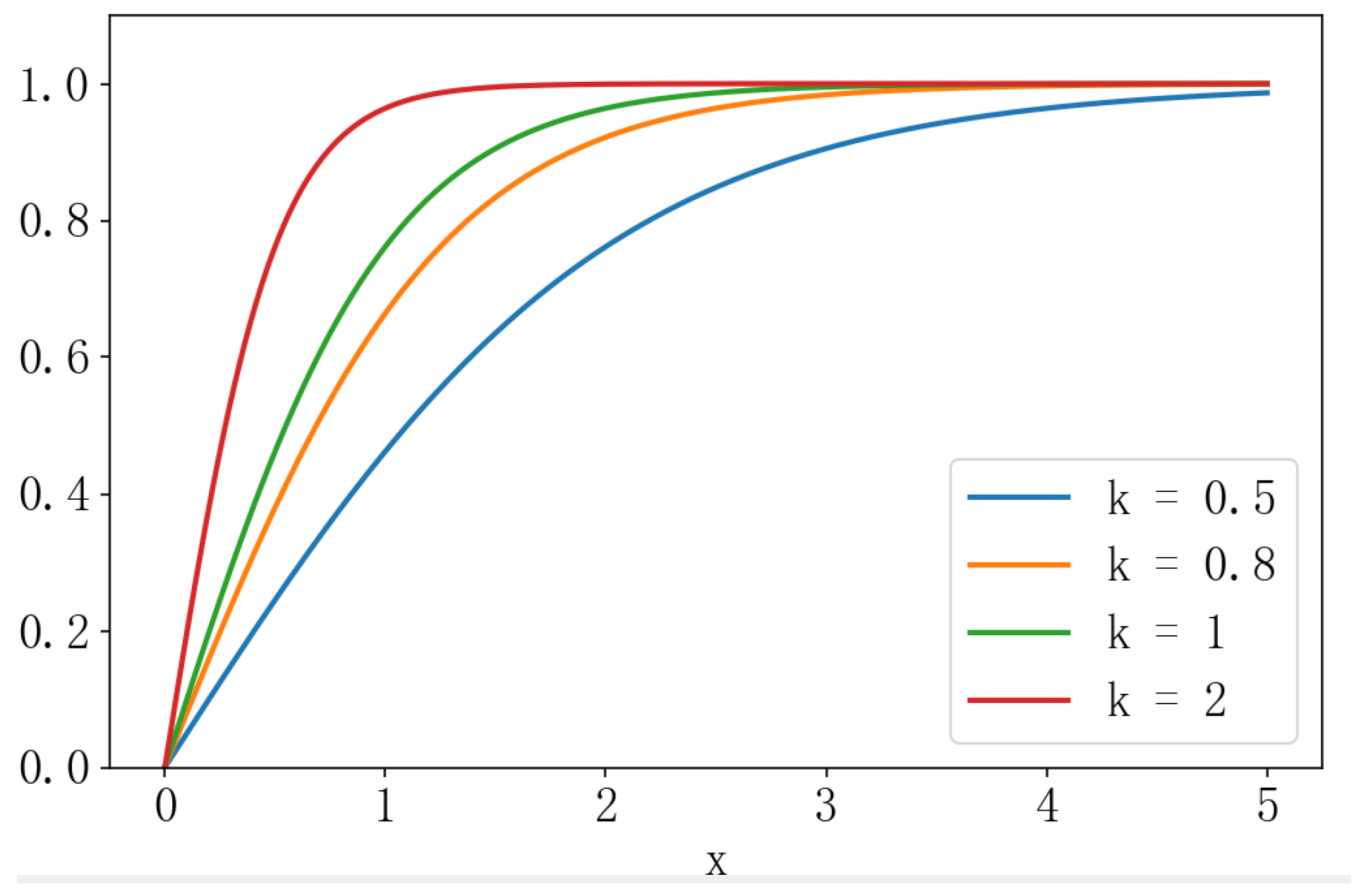
Figure 5.
Calculation of the number of times the direction of travel of vehicles changes at the point of conflict.
Figure 5.
Calculation of the number of times the direction of travel of vehicles changes at the point of conflict.

Figure 6.
PanoSim-Apollo co-simulation framework.
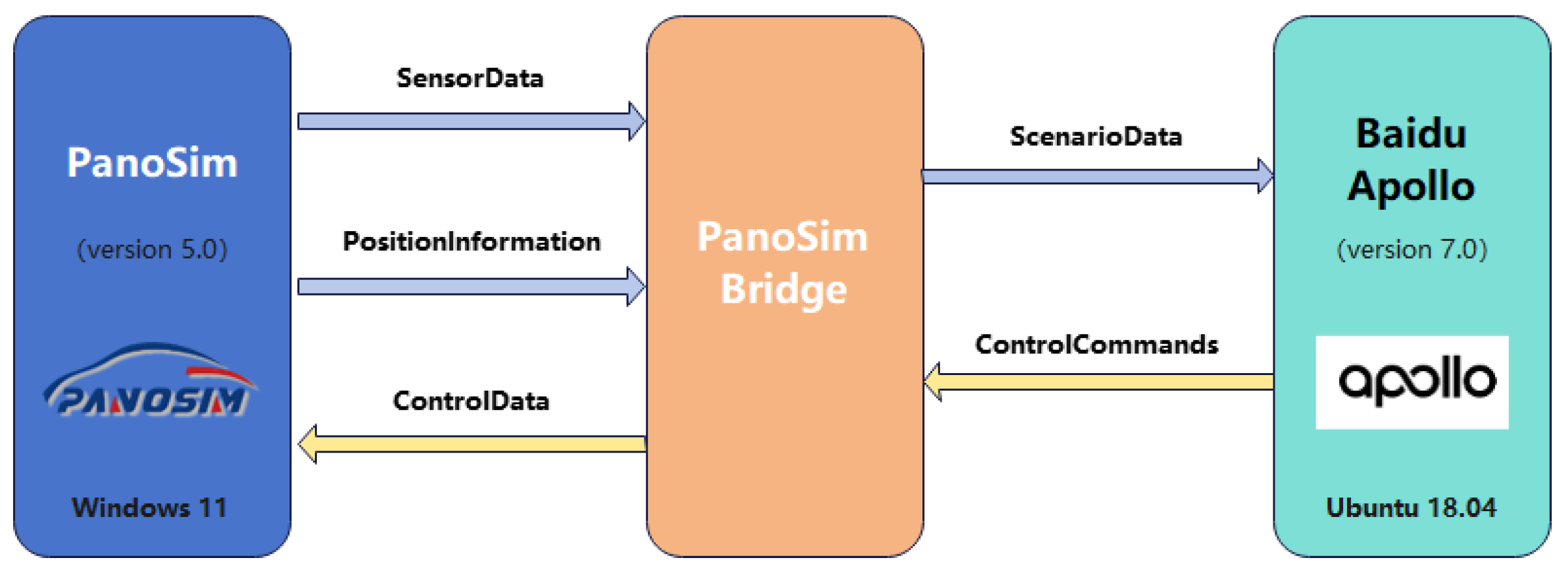
Figure 7.
PanoSim integrated simulation test platform.
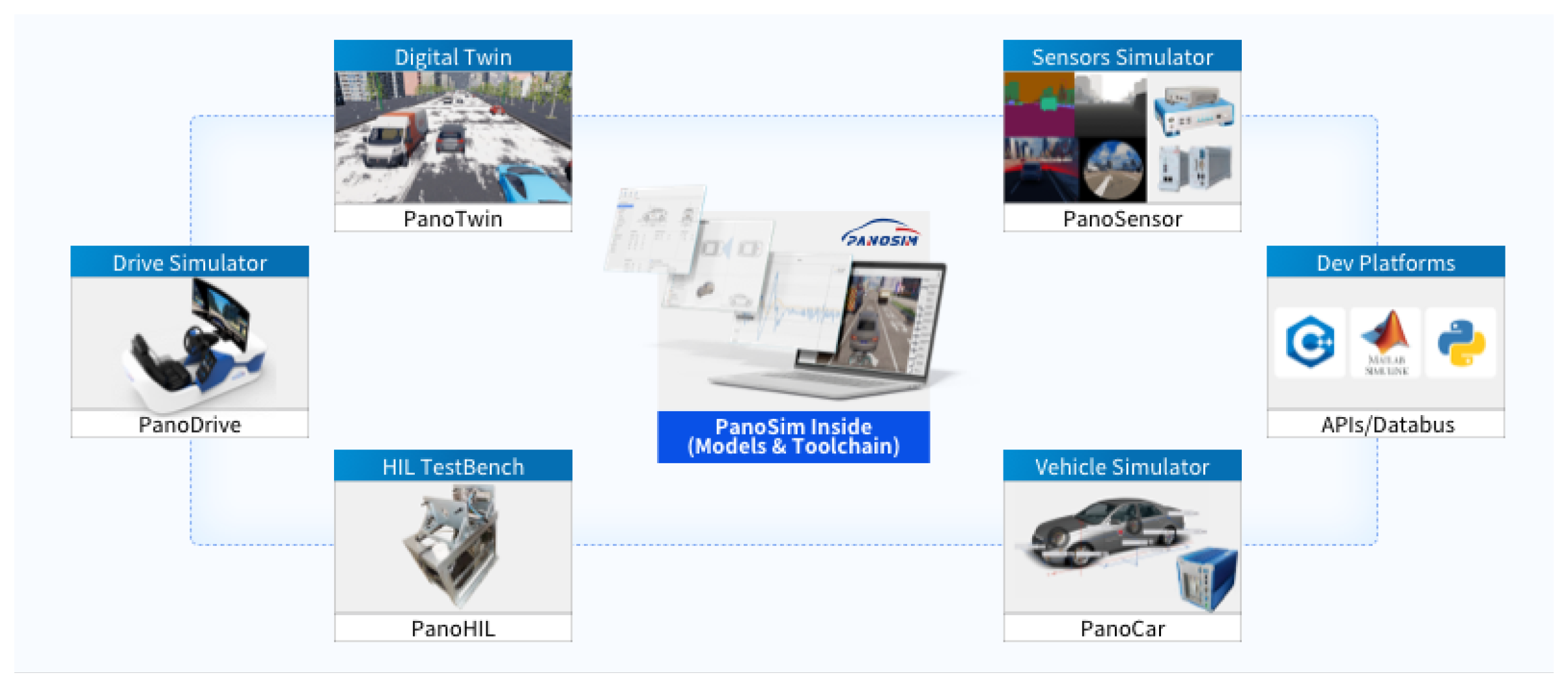
Figure 8.
Keyframe screenshots of scenario cases of varying complexity.
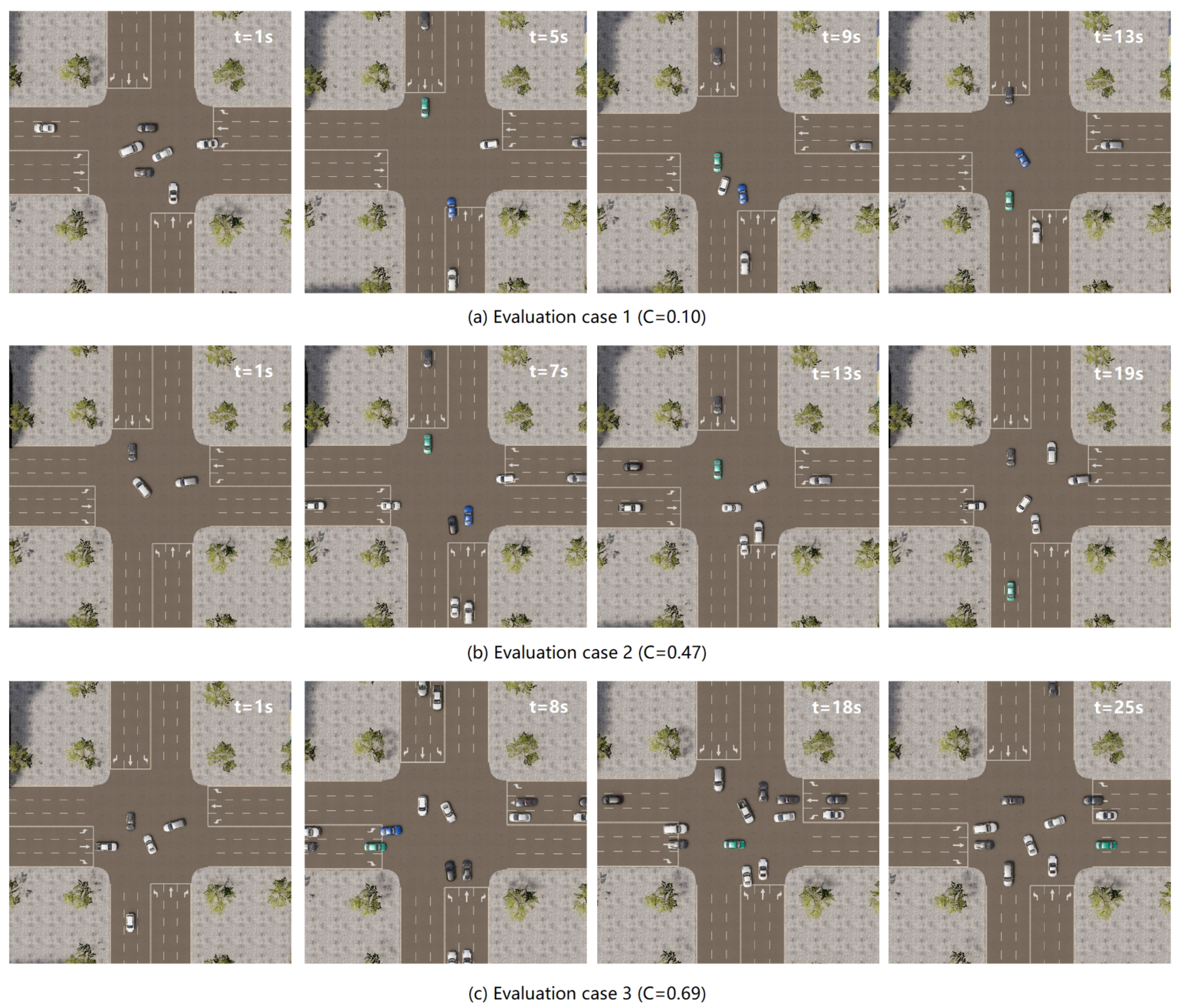
Figure 9.
Setting up of the unprotected left turn test experiment.
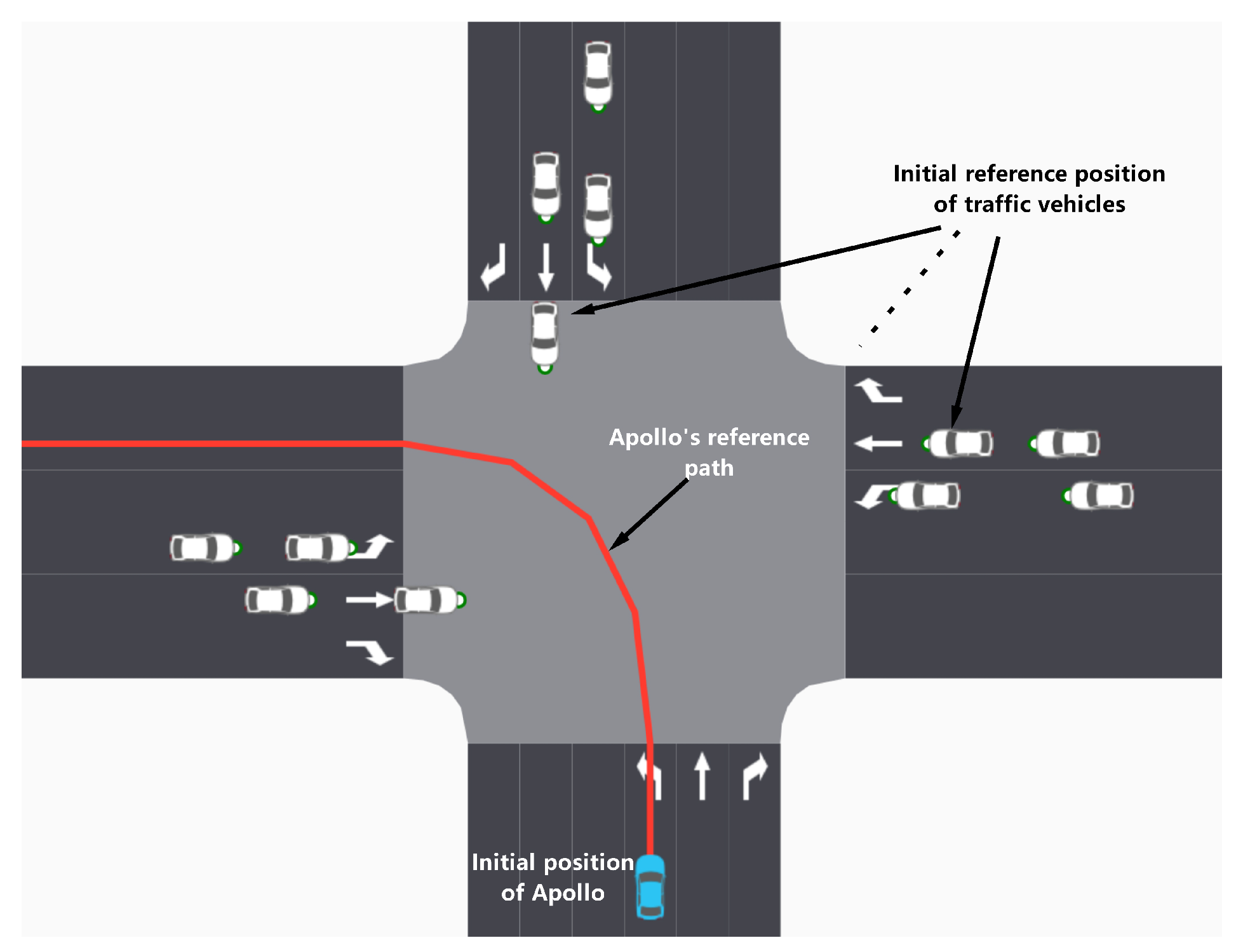
Figure 10.
Regression analysis results for complexity and risk.
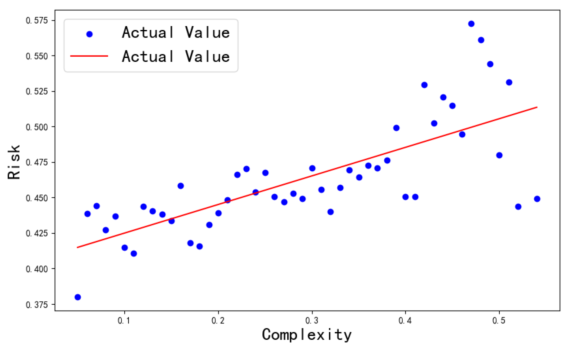
Figure 11.
Keyframe screenshots of the two Apollo test cases.
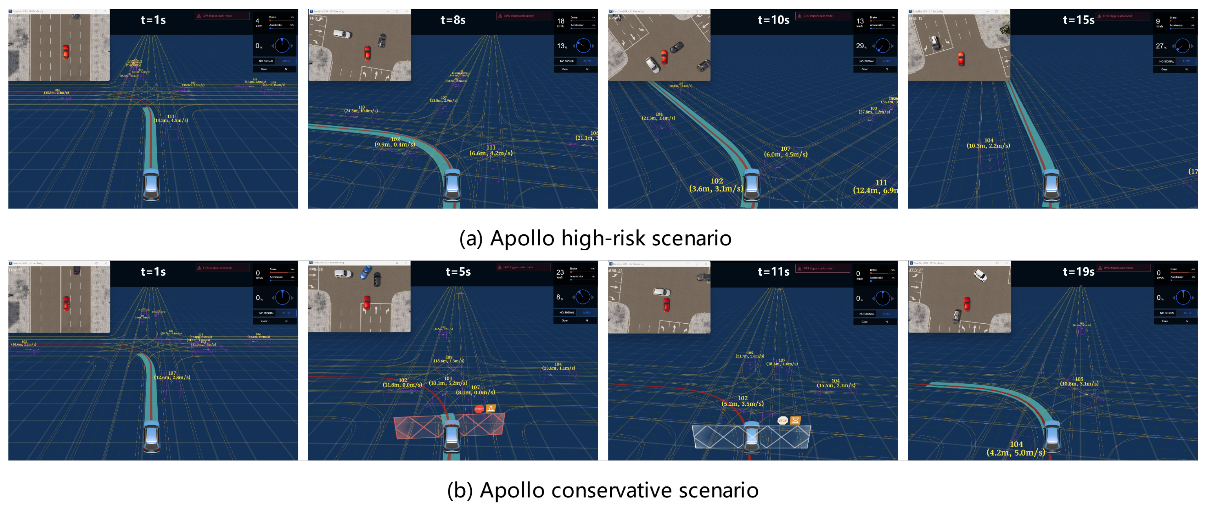
Figure 12.
Regression analysis results for complexity and efficiency.
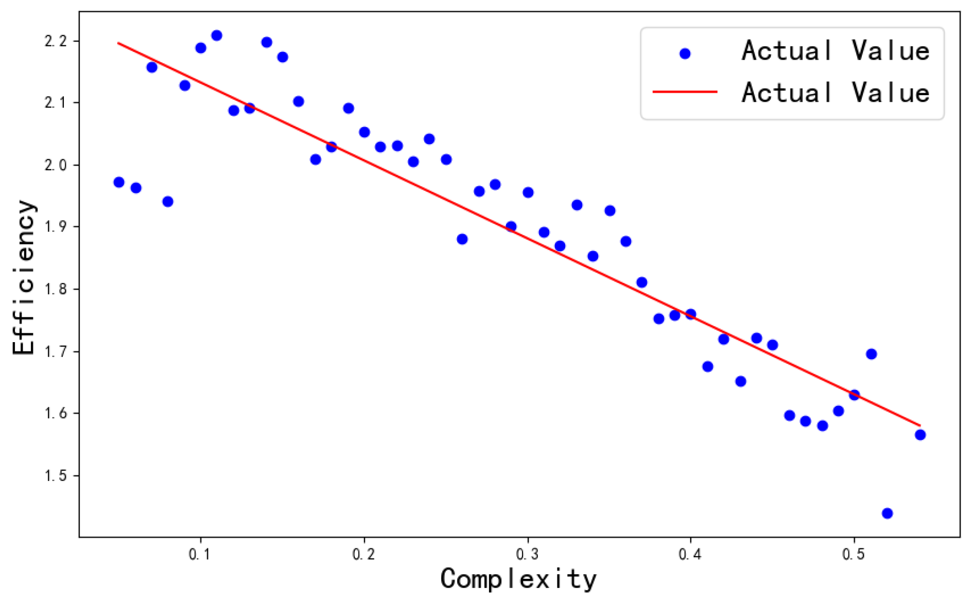
Figure 13.
This is a wide figure.
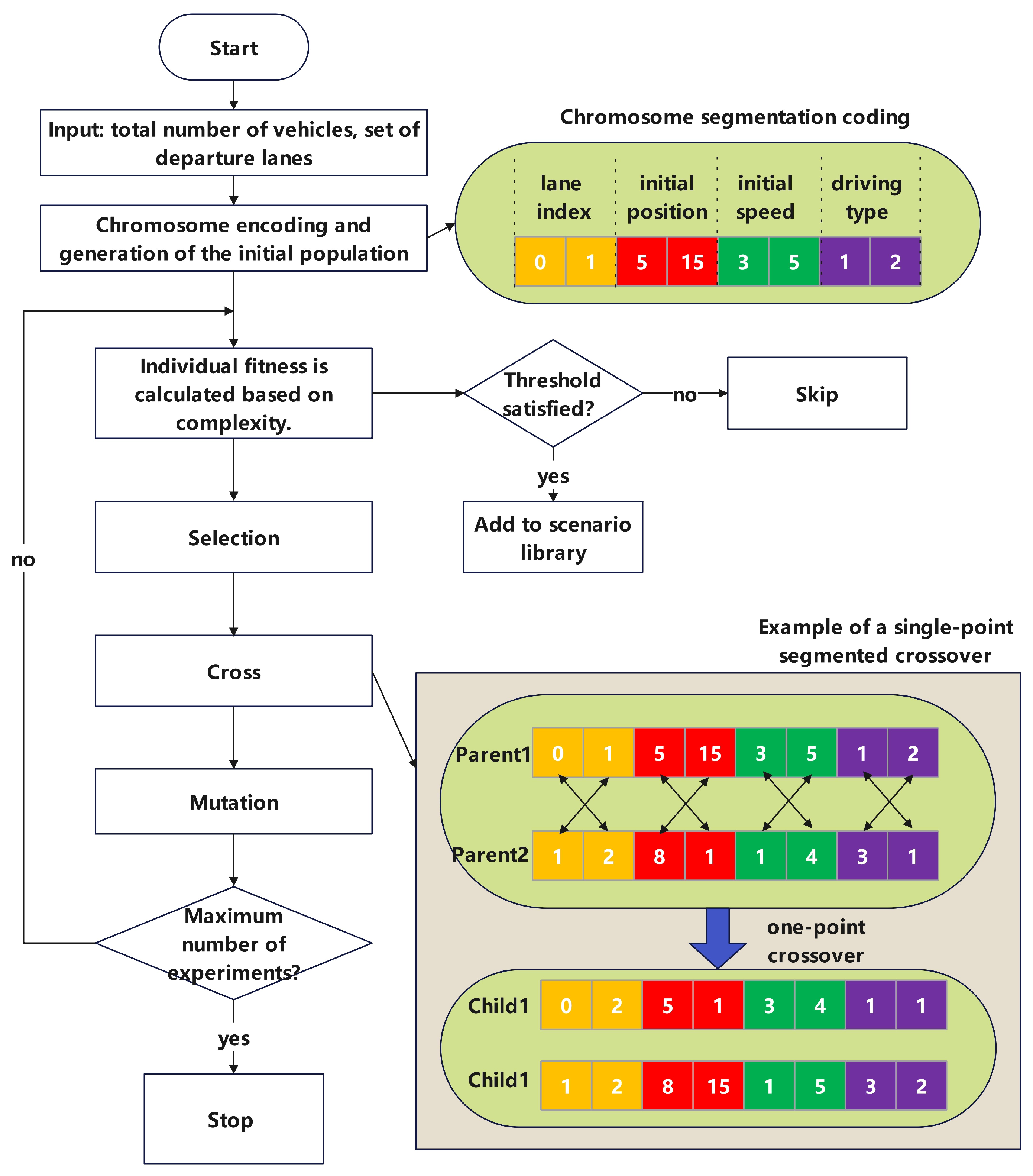
Figure 14.
The genetic algorithm-based optimization generation framework.

Figure 15.
Comparison of cumulative generation numbers for highly complex scenarios.
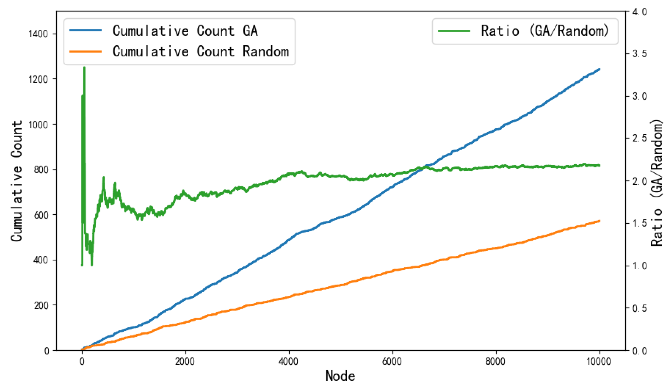

Table 1.
Statistical results of the validation set.
| Mean | Std | Min | Median | Max | |
|---|---|---|---|---|---|
| Complexity | 0.285 | 0.153 | 0.020 | 0.258 | 0.550 |
| Risk | 0.461 | 0.057 | 0.285 | 0.452 | 0.675 |
| Efficiency | 1.88 | 0.231 | 1.160 | 1.931 | 2.355 |
Table 2.
Correlation between Complexity and Risk, Efficiency.
| Risk | Efficiency | |
|---|---|---|
| r | 0.736 | -0.912 |
| p | 0.000 | 0.000 |
Table 3.
Validation of Regression Model and Parameter Estimates between Complexity and Risk
| Model | R | Adjusted | B | SE | t | p | |
|---|---|---|---|---|---|---|---|
| (Constant) | - | - | - | 0.405 | 0.009 | 46.493 | 0.000 |
| Complexity | 0.737 | 0.543 | 0.533 | 0.201 | 0.027 | 7.469 | 0.000 |
Table 4.
Validation of Regression Model and Parameter Estimates between Complexity and Efficiency.
| Model | R | Adjusted | B | SE | t | p | |
|---|---|---|---|---|---|---|---|
| (Constant) | - | - | - | 2.258 | 0.027 | 84.905 | 0.000 |
| Complexity | 0.912 | 0.832 | 0.828 | -1.255 | 0.082 | -15.249 | 0.000 |
Disclaimer/Publisher’s Note: The statements, opinions and data contained in all publications are solely those of the individual author(s) and contributor(s) and not of MDPI and/or the editor(s). MDPI and/or the editor(s) disclaim responsibility for any injury to people or property resulting from any ideas, methods, instructions or products referred to in the content. |
© 2024 by the authors. Licensee MDPI, Basel, Switzerland. This article is an open access article distributed under the terms and conditions of the Creative Commons Attribution (CC BY) license (http://creativecommons.org/licenses/by/4.0/).
Copyright: This open access article is published under a Creative Commons CC BY 4.0 license, which permit the free download, distribution, and reuse, provided that the author and preprint are cited in any reuse.


