Some Notes on the Gini Index and New Inequality Measures: The nth Gini Index

1. Introduction

The Gini index [1,2] is one of the principal inequality measures. It could be argued that it is the most well-known and widely accepted quantitative gauge in the field of economics and social sciences, used with the aim of quantifying income and wealth inequality [3,4,5,6]. A significant form of injustice is the unequal access to economic resources [7]. In this context, Gini coefficients are used as a primary summary measure of inequality by many government agencies and policy makers [8]. More generally, the Gini index is a quantitative measure of statistical evenness in the contex of non-negative datasets with positive means [9,10,11,12,13]. The Gini coefficient has been employed in a multitude of disciplines beyond its traditional applications in socioeconomics, where it is used to quantify inequality in wealth distributions. Its use has expanded to encompass a diverse range of scientific fields, including gender parity, access to education and health services, and environmental regulations [14]. The extant literature illustrates the extensive range of applications, with recent examples including: agriculture [15], anthropology [16], astrophysics [17], biomedical engineering [18], computational chemistry [19], criminology [20], ecology [21,22], econophysics [23], environmental sciences [24], epidemiology and public health [25,26],finance [27,28], geosciences and remote sensing [29], materials science and surface engineering [30], medical chemistry [31], molecular biology and genetics [32], population biology [33], sustainability science [34], and transportation [35].

Eliazar and Sokolov [36] presents an impressive toolbox of quantitative measures of societal egalitarianism. There is a plethora of inequality measures [37], and Charles et al. [38] points out that only two, the Gini index and Theil [39], satisfy the five most sought-after characteristics or properties, including the well-known transfer principle [40], the Gini index being more sensitive to income transfers towards the middle of the distribution [41]. In addition, the Gini index satisfies other essential conditions often imposed on any good poverty index [42].

The attractiveness of the Gini index often relies on the fact that it has an intuitive geometric interpretation, that is, it can be defined geometrically as the area between the line of perfect equality (the 45-degree line in the unit box) and the Lorenz curve multiplied by two. The Gini index is also interpreted in the context of interpersonal comparisons as the average gain to be expected, expressed as a proportion of the average level of income, if each member of the population is allowed to have the best income of either their own income or the income of another member of the population drawn at random [43]. Furthermore, this index is an important component of the Sen index of poverty intensity [44].

Regarding the computability of the Gini index, it has received some criticism: in Osberg [45] it is determined mathematically as the average of the absolute value of the relative mean difference in income between all possible pairs of individuals, in Liao [46] it is obtained directly from the Lorenz curve, Furman et al. [47] propose an alternative expression and interpretation of the Gini index based on the concept of a size-biased distribution, in [48] eight possible formulations of the Gini index are presented.

A profound connection between the Gini index and extreme value statistics is presented in [49]. The recent review by Eliazar [50] of the Gini coefficient as an elegant mathematical object sheds light on the Gini coefficient from a multitude of perspectives, culminating in a profound comprehension of the Gini coefficient that may potentially give rise to innovative applications in the realms of science and engineering. Multivariate extensions of the Gini index can be found in Lunetta1972 [51] and [52], who proposed a two-dimensional version, while Koshevoy and Mosler [53], Arnold [54] and Grothe et al. [55] extended it to more dimensions.

There are generally two different approaches to the analysis of the theoretical results of the Gini index: one is based on discrete distributions; the other on continuous distributions. These two approaches can be unified [56,57], but for certain purposes the continuous formulation, which is the one that will be followed in this paper, is more convenient, since it yields insights that are not easily accessible when the considered random variable is discrete [58].

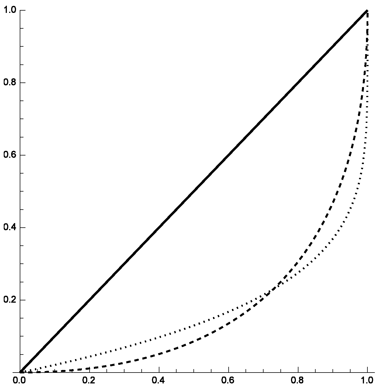
One of the major drawbacks of using the Gini index is that two distributions that behave differently in terms of their concentration (for example, through their Lorenz curves) can have the same value of this index. An illustrative example can be seen in Figure 1, which shows the Lorenz curves of two distributions, which will be revisited in Examples 3.5 and 3.6, that have the same Gini index. In these types of situations it is not possible to declare which distribution has a greater concentration using the Gini index, neither is it possible using the Lorenz curve, since neither dominates the other, but they do intersect. This problem has already been addressed in the literature on stochastic dominance [59] and inverse stochastic dominance [60]. Furthermore, the use of the square of the coefficient of variation is proposed in Gonzalez-Abril et al. [61], since it can be considered as an inequality measure similar to the Gini index. Liu and Gastwirth [8] mention that it is unrealistic to expect a single measure to describe the behaviour of an entire distribution with respect to inequality.

A whole family of inequality indices, called the nth Gini index, is proposed in this paper to overcome this situation, as opposed to the approach of combining the Gini index with another measure, as for example in Foster and Wolfson [62].

The rest of the paper is organized as follows. The Gini index is studied in Section 2. The generalizations of the Gini index are given in Section 3. Conclusions are drawn in the final section.

2. The Gini Index

Let $X\ge 0$ be a non-negative random variable with cumulative distribution function (cdf) $F\left(x\right)$ and probability density function $f\left(x\right)$, where $\mu =E\left[X\right]>0$ exists.

One of the most widely used definitions of the Gini index of the random variable X is [63]

$$IG\left(X\right)={\displaystyle \frac{E\left[\right|X_1-X_2\left|\right]}{2\mu }}$$

where $X_1,X_2$ are independent and identically distributed random variables with the same distribution as X. $E\left[\right|X_1-X_2\left|\right]$ is the mean difference and is denoted as $\Delta$ (that is, the Gini index is the relative mean difference). Nevertheless, $|X_1-X_2|=max\{X_1,X_2\}-min\{X_1,X_2\}$ and hence

$$IG\left(X\right)={\displaystyle \frac{E[max\{X_1,X_2\}-min\{X_1,X_2\}]}{2\mu }}={\displaystyle \frac{1}{\mu }}{\int }_0^{\infty }F\left(x\right)(1-F\left(x\right))dx$$

(1)

This result, which is also obtained in Section 3, was first given in Yitzhaki [64] when $support\left(X\right)\stackrel{\Delta }{=}\left\{x/f\left(x\right)>0\right\}=(a,b)$ with $-\infty <a<b<+\infty$.

This formulation is useful whenever the interpretation of the Gini index is related to extreme value theory, since it is established in terms of the difference between the maximum and the minimum (the most extreme values) of a random sample (see Yitzhaki and Schechtman [65] for more details).

The Gini index admits many other formulations and interpretations. By way of example, it is expressed below as an expected value of a transformation of X and also as the covariance between two transformations of X.

Given a non-negative random variable X, the transformation $Q^{*}\left(X\right)={\displaystyle \frac{1}{\mu }}{\int }_X^{\infty }(1-F\left(t\right))dt$ is considered, and its expected value is given by

$$\begin{array}{ccc}\hfill E\left[Q^{*}\left(X\right)\right]& =& {\displaystyle \frac{1}{\mu }}{\int }_0^{\infty }\left({\int }_x^{\infty }(1-F\left(t\right))dt\right)f\left(x\right)dx\hfill \\ & =& \left(\mathrm{by}\mathrm{integration}\mathrm{by}\mathrm{parts},u={\int }_x^{\infty }(1-F\left(t\right))dtanddv=f\left(x\right)dx\right)\hfill \\ & =& {\displaystyle \frac{1}{\mu }}\left({\left[F\left(x\right){\int }_x^{\infty }(1-F\left(t\right))dt\right]}_0^{\infty }+{\int }_0^{\infty }F\left(x\right)(1-F\left(x\right))dx\right)\hfill \\ & =& IG\left(X\right).\hfill \end{array}$$

Note that $E\left[{\int }_X^{\infty }(1-F\left(t\right))dt\right]={\int }_0^{\infty }F\left(x\right)(1-F\left(x\right))dx$. A better-known equality is $IG\left(X\right)=E[1-2Q(X\left)\right]$, where $Q\left(x\right)={\int }_0^{x}tf\left(t\right)dt$.

Let us examine another formulation of the Gini index. By integration by parts [66], with $u=F\left(x\right)(1-F(x\left)\right)$ and $dv=dx$,

$${\int }_0^{\infty }F\left(x\right)(1-F\left(x\right))dx={\left[xF\left(x\right)(1-F(x\left)\right)\right]}_0^{\infty }+2{\int }_0^{\infty }x(F\left(x\right)-{\displaystyle \frac{1}{2}})f\left(x\right)dx$$

and since ${lim}_{x\to \infty }x(1-F\left(x\right))=0$ and ${\int }_0^{\infty }x(F\left(x\right)-{\displaystyle \frac{1}{2}})f\left(x\right)dx=cov(X,F\left(X\right))$, due to $\mu <\infty$ and ${\mu }_{F\left(X\right)}={\displaystyle \frac{1}{2}}$, then

$$IG\left(X\right)={\displaystyle \frac{2}{\mu }}cov(X,F\left(X\right))=cov\left({\displaystyle \frac{X}{{\mu }_X}},{\displaystyle \frac{F\left(X\right)}{{\mu }_{F\left(X\right)}}}\right).$$

Therefore, the Gini index is the covariance between ${\displaystyle \frac{X}{{\mu }_X}}$ and ${\displaystyle \frac{F\left(X\right)}{{\mu }_{F\left(X\right)}}}$. Furthermore, this result can be used to obtain a well-known inequality between the Gini index and Pearson’s variation coefficient, denoted by $CV\left(X\right)$. From the equality $var\left(F\left(X\right)\right)={\displaystyle \frac{1}{12}}$ it follows that $co{v}^2(X,F\left(X\right))\le var\left(X\right)var\left(F\left(X\right)\right)={\displaystyle \frac{1}{12}}var\left(X\right)$ and, therefore

$$IG\left(X\right)\le \sqrt{{\displaystyle \frac{4}{12}}{\displaystyle \frac{var\left(X\right)}{{\mu }^2}}}={\displaystyle \frac{1}{\sqrt{3}}}CV\left(X\right).$$

On the other hand, if the linear regression between the variables X and $F\left(X\right)$ is considered, that is $X=a+bF\left(X\right)$, then the regression coefficient b is $b=6\mu IG\left(X\right)$. This expression allows the Gini index to be easily obtained by employing any software to carry out the linear regression between the variables X and $F\left(X\right)$.

3. The nth Gini Index

Let $X_1,X_2,\cdots ,X_n$ be independent and identically distributed (iid) random variables with the same distribution as X. If the transformations given by $U_n=max\left\{X_1,X_2,\cdots ,X_n\right\}$ and $V_n=min\left\{X_1,X_2,\cdots ,X_n\right\}$ are considered, then their cdf’s are: $F_{U_n}\left(u\right)=F{\left(u\right)}^n$ and $F_{V_n}\left(v\right)=1-{(1-F\left(v\right))}^n$, and $0\le V_n\le U_n$ for each integer n. Hence,

$$0\le E\left[V_n\right]\le E\left[U_n\right]={\int }_0^{\infty }xnF{\left(x\right)}^{n-1}f\left(x\right)dx\le n{\int }_0^{\infty }xf\left(x\right)dx=n\mu$$

that is, $E\left[U_n\right]$ and $E\left[V_n\right]$ exist, and therefore $E[U_n-V_n]$ exists for any n.

By using $E\left[X\right]={\int }_0^{\infty }(1-F\left(x\right))dx$, then $E\left[U_n\right]={\int }_0^{\infty }(1-F{\left(x\right)}^n)dx$ and $E\left[V_n\right]={\int }_0^{\infty }{(1-F\left(x\right))}^{n}dx$. Thus, for any integer:

$$E[U_n-V_n]={\int }_0^{\infty }(1-F{\left(x\right)}^n-{(1-F\left(x\right))}^n)dx.$$

Let us denote $a_n=E[U_n-V_n]$ and study the sequence $\left\{a_n\right\}$.

Clearly, this sequence is non-negative and non-decreasing since $E\left[U_{n+1}\right]\ge E\left[U_n\right]$ and $E\left[V_{n+1}\right]\le E\left[V_n\right]$. Furthermore, $E[U_n-V_n]\le {\displaystyle \frac{n}{2}}\Delta ={\displaystyle \frac{n}{2}}E[U_2-V_2]$ as can be seen in the following result.

Proposition 3.1. 

Let $X_1,X_2,\cdots ,X_n$ be iid with cdf $F\left(x\right)$, then

$$E[U_n-V_n]\le n{\int }_0^{\infty }F\left(x\right)(1-F\left(x\right))dx,\mathrm{for}n\ge 2$$

(2)

and if $n=2$ or 3, then the equality holds.

Proof: Let us find a bound of $a_n$ by induction:

For $n=2$: $a_2={\int }_0^{\infty }(1-F{\left(x\right)}^2-{(1-F\left(x\right))}^2)dx=2{\int }_0^{\infty }F\left(x\right)(1-F\left(x\right))dx$

For $n=3$: $a_3={\int }_0^{\infty }(1-F{\left(x\right)}^3-{(1-F\left(x\right))}^3)dx=3{\int }_0^{\infty }F\left(x\right)(1-F\left(x\right))dx$

For $n+1$$(n\ge 3)$:

$$\begin{array}{ccc}\hfill a_{n+1}-a_n& =& {\int }_0^{\infty }(F{\left(x\right)}^n-F{\left(x\right)}^{n+1}+{(1-F\left(x\right))}^n-{(1-F\left(x\right))}^{n+1})dx\hfill \\ & =& {\int }_0^{\infty }{(F\left(x\right)}^n(1-F\left(x\right))+{(1-F\left(x\right))}^n(1-(1-F\left(x\right)))dx\hfill \\ & =& {\int }_0^{\infty }F\left(x\right)(1-F\left(x\right))(F{\left(x\right)}^{n-1}+{(1-F\left(x\right))}^{n-1})dx\hfill \\ & \le & {\int }_0^{\infty }F\left(x\right)(1-F\left(x\right))dx\hfill \end{array}$$

since $0\le (x^n+{(1-x)}^n)\le {(x+(1-x))}^n=1$ when $0\le x\le 1$ for each integer n. Therefore $a_{n+1}\le a_n+{\int }_0^{\infty }F\left(x\right)(1-F\left(x\right))dx$, and by induction $a_{n+1}\le a_2+(n-1){\int }_0^{\infty }F\left(x\right)(1-F\left(x\right))dx$, and the proof is complete. ▪

Note that the inequality (2) is also true if $n=1$ since $U_1=V_1$ and therefore

$$0=a_1\le {\int }_0^{\infty }F\left(x\right)(1-F\left(x\right))dx<{\int }_0^{\infty }(1-F\left(x\right))dx=\mu$$

(3)

Another important result which must also be borne in mind is presented.

Proposition 3.2. 

Let X be a non-negative random variable with $\mu >0$. The sequence ${\left\{{\displaystyle \frac{1}{n}}E[U_n-V_n]\right\}}_{n=3}^{\infty }$ is non-increasing and tends towards zero.

Proof: From Proposition 3.1:

$$a_{n+1}-a_n={\int }_0^{\infty }{(F\left(x\right)}^n(1-F\left(x\right))+{(1-F\left(x\right))}^n(1-(1-F\left(x\right)))dx$$

On the other hand:

$$1={(x+(1-x))}^{n+1}=x^{n+1}+(n+1)x^n(1-x)+R\left(x\right)+(n+1)x{(1-x)}^n+{(1-x)}^{n+1}$$

where $R\left(x\right)\ge 0$ if $0\le x\le 1$ and $n\ge 3$, and hence

$$x^n(1-x)+x{(1-x)}^n\le {\displaystyle \frac{1}{n+1}}\left(1-x^{n+1}-{(1-x)}^{n+1}\right)$$

Therefore:

$$a_{n+1}-a_n\le {\displaystyle \frac{1}{n+1}}{\int }_0^{\infty }\left(1-F{\left(x\right)}^{n+1}-{(1-F\left(x\right))}^{n+1}\right)dx={\displaystyle \frac{1}{n+1}}{a}_{n+1}$$

which implies that ${\displaystyle \frac{1}{n+1}}{a}_{n+1}\le {\displaystyle \frac{1}{n}}{a}_n$ and therefore $\left\{{\displaystyle \frac{a_n}{n}}\right\}$ is non-increasing. In fact, if $V_{n+1}=X_{\left(1\right)}\le X_{\left(2\right)}\cdots \le X_{\left(n\right)}\le X_{(n+1)}=U_{n+1}$ are the order statistics, then it is easy to prove that ${\displaystyle \frac{E\left[U_{n+1}\right]}{n+1}}={\displaystyle \frac{E\left[U_n\right]}{n}}-{\displaystyle \frac{1}{n(n+1)}}E\left[X_{\left(n\right)}\right]$, ${\displaystyle \frac{E\left[V_{n+1}\right]}{n+1}}={\displaystyle \frac{E\left[V_n\right]}{n}}-{\displaystyle \frac{1}{n(n+1)}}E\left[X_{\left(2\right)}\right]$, and hence ${\displaystyle \frac{a_{n+1}}{n+1}}-{\displaystyle \frac{a_n}{n}}={\displaystyle \frac{-1}{n(n+1)}}\left(E\left[X_{\left(n\right)}\right]-E\left[X_{\left(2\right)}\right]\right)\le 0$.

On the other hand, as $\left\{{\displaystyle \frac{a_n}{n}}\right\}$ is non-increasing and $0\le a_n$ for all n, then $g={lim}_{n\to \infty }{\displaystyle \frac{a_n}{n}}$ exists.

Let us see that $g=0$:

If $support\left(X\right)\stackrel{\Delta }{=}\left\{x/f\left(x\right)>0\right\}\subset [0,b]$ where b is a constant then $a_n\le b$, and therefore $0\le {\displaystyle \frac{a_n}{n}}\le {\displaystyle \frac{b}{n}}\to 0$ if $n\to \infty$.

If $support\left(X\right)=(0,\infty )$ then $0\le F\left(x\right)<1$ for all x. Hence:

$$0\le {\displaystyle \frac{a_n}{n}}\le {\displaystyle \frac{E\left[U_n\right]}{n}}={\int }_0^{\infty }xF{\left(x\right)}^{n-1}f\left(x\right)dx$$

and by taking the limit when n tends towards ∞, and since the integral is positive then:

$$\underset{n\to \infty }{lim}{\displaystyle \frac{a_n}{n}}\le \underset{n\to \infty }{lim}{\int }_0^{\infty }xF{\left(x\right)}^{n-1}f\left(x\right)dx={\int }_0^{\infty }xf\left(x\right)\left(\underset{n\to \infty }{lim}F{\left(x\right)}^{n-1}\right)dx=0$$

and the proof is complete. ▪

A family of indices of X is defined from the properties of $E[U_n-V_n]$ as follows:

Definition 3.3. 

Let X be a non-negative random variable with $\mu >0$. For each integer n, the nth Gini index of X is defined as follows:

$$I{G}_n\left(X\right)={\displaystyle \frac{E[U_n-V_n]}{n\mu }},forn\ge 2.$$

(4)

Let us enumerate some properties of the nth Gini index:

• The nth Gini index exists for any non-negative random variable with $\mu >0$. This property is of major significance because if X is an income distribution with $\mu >0$, then the nth Gini index can always be calculated even if some of its conventional moments do not exist.
• $IG\left(X\right)=I{G}_2\left(X\right)=I{G}_3\left(X\right)$.
• $0\le I{G}_n\left(X\right)<1$ for all $n>3$ (from Proposition 3.1 and inequality (3)).
• $I{G}_n\left(bX\right)=I{G}_n\left(X\right)$ for any $b>0$, that is, the nth Gini index is not affected by ratio-scale changes of the X variable.
• $I{G}_n(a+X)={\displaystyle \frac{\mu }{a+\mu }}I{G}_n\left(X\right)$ if $Y=a+X$ is a non-negative random variable (translation-scale changes). Therefore, transforming X into $a+X$ with $a>0$ diminishes the nth Gini index.
• $I{G}_n\left(X\right)={\displaystyle \frac{1}{\mu }}Cov\left(X,F_{U_n}\left(X\right)-F_{V_n}\left(X\right)\right)$, that is, the nth Gini index is the covariance between X and a transformation of X.
• The sequence ${\left\{I{G}_n\left(X\right)\right\}}_{n=3}^{\infty }$ is non-increasing and ${lim}_{n\to \infty }I{G}_n\left(X\right)=0$. (straightforward from Proposition 3.2).

Proposition 3.4. 

Let X be a non-negative random variable with $\mu >0$. For each integer n, a value $r_n$ exists such that $I{G}_n\left(X\right)=IG(r_n+X)$.

Proof: Let $g=I{G}_n\left(X\right)$, and by taking into consideration that $0<g\le IG\left(X\right)$ (if $g=0$ then $IG\left(X\right)=0$) then the following equation in terms of r is considered: $I{G}_n\left(X\right)={\displaystyle \frac{\mu }{r+\mu }}IG\left(X\right)$, whose solution is given by $r_n=\mu \left({\displaystyle \frac{IG\left(X\right)}{g}}-1\right)\ge 0$. Therefore, the Gini index of the random variable $Y=r_n+X$ is equal to $I{G}_n\left(X\right)$. ▪

The most important consequence of Proposition 3.4 is that the nth Gini index is a Gini index and can be interpreted in this way.

One of major drawbacks when the Gini index is utilized, is the fact that there are non-negative random variables X and Y such that $IG\left(X\right)=IG\left(Y\right)$ and, therefore, it is not possible using the Gini index to quantify which distribution is more unequal. To overcome this situation, the nth Gini index can be calculated for several values of n. Let us consider an example based on two significant parametric models for describing incomes, whose Lorenz curves can be seen in Figure 1.

Example 3.5. 

Let $X\sim SM(q=2,a=1,b=1)$ be a Singh-Maddala distribution with shape parameters q and a, and scale parameter b. By using any calculus program, it can be calculated that

$$\begin{array}{cc}\hfill {\left\{I{G}_n\left(X\right)\right\}}_{n=2}^{10}& =\left\{{\displaystyle \frac{2}{3}},{\displaystyle \frac{2}{3}},{\displaystyle \frac{22}{35}},{\displaystyle \frac{62}{105}},{\displaystyle \frac{386}{693}},{\displaystyle \frac{122}{231}},{\displaystyle \frac{3238}{6435}},{\displaystyle \frac{3098}{6435}},{\displaystyle \frac{106762}{230945}}\right\}\hfill \end{array}$$

(5)

$$\begin{array}{cc}& =\left\{\stackrel{⌢}{0.6},\stackrel{⌢}{0.6},0.6286,0.5905,0.5570,0.5281,0.5032,0.4814,0.4622\right\}\hfill \end{array}$$

(6)

On the other hand, let $Y\sim Pa(k={\displaystyle \frac{1}{5}},\alpha ={\displaystyle \frac{5}{4}})$ be a Pareto distribution with minimum value parameter k and shape parameter α. It can be obtained that

$$\begin{array}{cc}\hfill {\left\{I{G}_n\left(Y\right)\right\}}_{n=2}^{10}& =\left\{{\displaystyle \frac{2}{3}},{\displaystyle \frac{2}{3}},{\displaystyle \frac{57}{88}},{\displaystyle \frac{83}{132}},{\displaystyle \frac{14701}{24024}},{\displaystyle \frac{2391}{4004}},{\displaystyle \frac{372893}{638352}},{\displaystyle \frac{45691}{79794}},{\displaystyle \frac{9402119}{16721276}}\right\}\hfill \end{array}$$

(7)

$$\begin{array}{cc}& =\left\{\stackrel{⌢}{0.6},\stackrel{⌢}{0.6},0.6477,0.6288,0.6119,0.5972,0.5841,0.5726,0.5623\right\}\hfill \end{array}$$

(8)

Note that $IG\left(X\right)=IG\left(Y\right)$ and therefore these two distributions cannot be compared in relation to their concentration using the Gini index, neither can their Lorenz curves be used for that purpose because, as shown in Figure 1, there is no dominance relation, but they do intersect. Since $I{G}_n\left(X\right)<I{G}_n\left(Y\right)$ for $n\ge 4$, then the $Pa(k={\displaystyle \frac{1}{5}},\alpha ={\displaystyle \frac{5}{4}})$ distribution can be considered to be more concentrated than the $SM(q=2,a=1,b=1)$ distribution, despite having the same value for the Gini index.

It is easy to make two variables take the same Gini index by means of a positive shift of the variable that has the greatest Gini index. Let X and Y be non-negative random variables with $IG\left(X\right)>IG\left(Y\right)$. As in Proposition 3.4, it is possible to find a value $r^{*}$ such that $IG(r^{*}+X)=IG\left(Y\right)$. Therefore, the two random variables $r^{*}+X$ and Y are similar from the point of view of their concentration. Note that no particular supposition about the distribution has been made.

In Forcina and Giorgi [67] is pointed out that the political and economic debate on how to achieve a more equal distribution of income and wealth was particularly lively at the beginning of the last century. Proposition 3.2 provides us with a statistical way to attain perfect equality, that is, if no economic nor any other kind of consideration is made, then the perfect equality of a distribution X is attained by considering the shifted variables $X_n=r_n+X$ such that $IG\left(X_n\right)=I{G}_n\left(X\right)$.

Example 3.6. 

Let X be a Singh-Maddala distribution $SM(q=2,a=1,b=1)$. The first values of $I{G}_n\left(X\right)$ are given in Example 3.5. Thus, the values $r_n$ such that $IG(r_n+X)=I{G}_n\left(X\right)$ are $r_n=\left\{{\displaystyle \frac{2}{33}},{\displaystyle \frac{4}{31}},{\displaystyle \frac{38}{193}},{\displaystyle \frac{16}{61}},{\displaystyle \frac{526}{1619}},{\displaystyle \frac{596}{1549}},{\displaystyle \frac{70802}{160143}}\right\}$ for $n=4,\cdots ,10$. Therefore, perfect equality is achieved with the sequence of random variables $X_n=X_{n-1}+b_n$, where $b_n=\left\{{\displaystyle \frac{2}{33}},{\displaystyle \frac{70}{1023}},{\displaystyle \frac{406}{5983}},{\displaystyle \frac{770}{11773}},{\displaystyle \frac{6182}{98759}},{\displaystyle \frac{150150}{2507831}},{\displaystyle \frac{14227070}{248061507}}\right\}$ for $n=4,\cdots ,10$. Hence, the initial concentration measured through the Gini index, which has a value equal to $I{G}_3\left(X\right)=2/3\simeq 0.67$, is reduced to $I{G}_{10}\left(X\right)\simeq 0.46$ through the seven successive increases given by $b_n$, which means a decrease of 31%.

3.1. The Extended Gini Index, the Lorenz Family and the $uv$-Gini Index

A similar generalization of the Gini index is given in Yitzhaki [68] and its development is given in Yitzhaki and Schechtman [58] which is called extended Gini or S-Gini index in the mathematically oriented literature. This family of indices, denoted by $EG(X,v)$, is defined as

$$EG(X,v)={\displaystyle \frac{1}{\mu }}{\int }_0^{\infty }\left(1-F\left(x\right)-{(1-F\left(x\right))}^v\right)dx$$

(9)

where1 $v\ge 1$. Several authors suggest using the extended Gini index to characterize the distribution [69].

Hence, $EG(X,v)={\displaystyle \frac{1}{\mu }}\left(E\left[X\right]-E[min\left\{X_1,X_2,\cdots ,X_v\right\}]\right)$ if v is an integer. Note that $E[U_2-V_2]={\int }_0^{\infty }(1-F{\left(x\right)}^2-{(1-F\left(x\right))}^2)dx=2{\int }_0^{\infty }(1-F\left(x\right)-{(1-F\left(x\right))}^2)dx$, and therefore, $IG\left(X\right)=EG(X,2)=I{G}_2\left(X\right)$.

By following a similar expression of (9), a generalization of the nth Gini index is proposed by considering two positive real numbers instead of an integer as in (4):

Definition 3.7. 

Let X be a non-negative random variable with $\mu >0$. For two positive real numbers $u,v\ge 1$, the $uv$-Gini index of X is defined as follows:

$$IG(X,u,v)={\displaystyle \frac{1}{u\mu }}{\int }_0^{\infty }\left(1-F{\left(x\right)}^u-{(1-F\left(x\right))}^v\right)dx,foru,v\ge 1$$

(10)

This index is more general than the extended Gini since $EG(X,v)=IG(X,1,v)$.

It is well-known from the economic literature that the basic condition for a measure of inequality is that it should satisfy the Pigou-Dalton principle of transfers or eventually a similar normative principle. We now show that the $uv$-Gini index satisfies this principle from rank-dependent inequality measurements.

It is interesting to observe that the $uv$-Gini index is a linear combination of indices that belong to two alternative families of rank-dependent measures of inequality. One of these families is the generalized Gini family introduced by Kakwani [70], Donaldson and Weymark [71], and later by Yitzhaki [68]. This family is defined by

$$G(X,v)=1-{\displaystyle \frac{1}{\mu }}{\int }_0^{\infty }{\left(1-F\left(x\right)\right)}^{v}dx,forv\ge 1,$$

(11)

and it is identical to expression (9).

The second family, the Lorenz family of inequality measures, was introduced in Aaberge [72] and is defined by

$$D(X,u)={\displaystyle \frac{1}{u\mu }}{\int }_0^{\infty }F\left(x\right)\left(1-F{\left(x\right)}^u\right)dx,foru\ge 1.$$

(12)

Hence, by inserting (11) and (12) into $IG(X,u,v)$ (defined by (10)), it follows that

$$uIG(X,u,v)=(u-1)D(X,u-1)+G(X,v),foru,v\ge 1$$

and, therefore,

$$IG(X,u,v)=(1-{\displaystyle \frac{1}{u}})D(X,u-1)+{\displaystyle \frac{1}{u}}G(X,v),\mathrm{for}u,v\ge 1.$$

(13)

It follows directly from expression (13) that the $uv$-Gini index is a convex combination of $G(x,v)$ and $D(X,u)$. Thus, since $G(x,v)$ and $D(X,u)$ satisfy the Pigou-Dalton principle of transfers, it follows from (13) that $IG(X,u,v)$ also satisfies the Pigou-Dalton principle of transfers. Furthermore, by observing that $G(x,v)$ and $D(X,u)$ are (0,1)-normalized measures of inequality, it holds that $IG(X,u,v)$ is also a (0,1)-normalized measure, and takes its maximum value when one unit receives the total income and its minimum value when all the units receive the same income.

3.2. The nth Gini Index in Terms of the Lorenz Curve

Taking into consideration that $I{G}_n\left(X\right)=IG(X,n,n)$, it follows that the nth Gini index verifies the Pigou-Dalton principle of transfers and that this index assumes the maximum value in the case of maximum concentration.

It is straightforward to write $IG(X,n,n)$ in terms of the Lorenz curve from (13) and the Lorenz curve expression of $G(X,n)$ and $D(X,n)$.

The Lorenz curve $L(·)$ for X is defined by $L\left(u\right)={\displaystyle \frac{1}{\mu }}{\int }_0^{u}xdF\left(x\right)$ for any $0\le u\le 1$, and it can be observed in Yitzhaki [68] and Aaberge [72] that

$$G(X,n)=n(n-1){\int }_0^1{(1-u)}^{n-2}(u-L\left(u\right))du,D(X,n)=(n+1){\int }_0^1{u}^{n-1}(u-L\left(u\right))du,$$

therefore

$$I{G}_n\left(X\right)=(n-1){\int }_0^1\left(u^{n-2}+{(1-u)}^{n-2}\right)(u-L\left(u\right))du.$$

Hence, in order to be more operative since $I{G}_2\left(X\right)=I{G}_3\left(X\right)=IG\left(X\right)$, it can be defined

$$I{G}_n^{*}\left(X\right)=(n+1){\int }_0^1\left(u^n+{(1-u)}^n\right)(u-L\left(u\right))du,n=1,2,3,\cdots$$

(14)

It can be seen that the criterion of Lorenz-dominance, which recognizes the highest of the Lorenz curves as preferable [73], is verified for the family $I{G}_n^{*}\left(X\right)$ from (14). Nevertheless, due to fact that the Lorenz curves may intersect, the criterion of Lorenz-dominance does not apply in many practical situations. No single measure is able to retain all the features concerning inequality exhibited by the Lorenz curve. For this reason, it is proposed that the first few nth indices $I{G}_n^{*}\left(X\right)$ are obtained together with other possible measures for the purpose of application.

4. Conclusions

In this paper, a new family of inequality indices, the nth Gini index, is proposed and studied. These indices are based on the deviation between the expected maximum and the expected minimum of independent and identically distributed random samples. This family generalizes the Gini index. At the same time, these indices and the S-Gini index are generalized by proposing the $uv-$Gini index, which turns out to be a convex combination of the S-Gini index and the Lorenz family of inequality measures, thereby verifying the principle of transfers. These new formulations can be useful whenever the preferred interpretation is related to extreme value theory and the use of a few measures of this family of Gini indices is proposed to obtain a summary of the basic information provided by the Lorenz curve.

This family of Gini indices enables a path to be found to the perfect equality for a given distribution of incomes through successive and equal increases of the incomes of each individual. It is also specially useful to compare the concentration of two distributions that have the same Gini index and intersecting Lorenz curves.

References

- Gini, C. Sulla misura della concentrazione e della variabilità dei caratteri. Atti del Reale Istituto Veneto di Scienze, Lettere ed Arti 1914, 73, 1203–1248. Reprinted in: C. Gini, (2005). On the measurement of concentration and variability of characters. Metron - International Journal of Statistics 63, 3-38.
- Gini, C. Measurement of inequality of incomes. The Economic Journal 1921, 31, 124–126. [Google Scholar] [CrossRef]
- Karsu, Ö.; Morton, A. Inequity averse optimization in operational research. European Journal of Operational Research 2015, 173, 343–359. [Google Scholar] [CrossRef]
- Giorgi, G.; Gigliarano, C. The Gini concentration index: a review of the inference literature. Journal of Economic Surveys 2016, 31, 1130–1148. [Google Scholar] [CrossRef]
- Wu, W.C.; Chang, Y.T. Income inequality, distributive unfairness, and support for democracy: evidence from East Asia and Latin America. Democratization 2019, 26, 1475–1492. [Google Scholar] [CrossRef]
- Giorgi, G. , Gini Coefficient. In In: P. Atkinson, S. Delamont, A. Cernat, J.W. Sakshaug, and R.A. Williams; SAGE Research Methods Foundations, 2020. [CrossRef]
- Atkinson, A. Inequality; Harvard University Press, 2015.
- Liu, Y.; Gastwirth, J. On the capacity of the Gini index to represent income distributions. METRON 2020, 78, 61–69. [Google Scholar] [CrossRef]
- Xu, K. How has the Literature on Gini’s Index Evolved in the Past 80 Years? Economics working paper, Dalhousie University, Canada, 2004.
- Farris, F. The Gini Index and Measures of Inequality. American Mathematical Monthly 2010, 117, 851–864. [Google Scholar] [CrossRef]
- Eliazar, I. Harnessing inequality. Physics Reports 2016, 649, 1–29. [Google Scholar] [CrossRef]
- Eliazar, I. A tour of inequality. Annals of Physics 2018, 389, 306–332. [Google Scholar] [CrossRef]
- Eliazar, I.; Giorgi, G. From Gini to Bonferroni to Tsallis: an inequality-indices trek. METRON 2020, 78, 119–153. [Google Scholar] [CrossRef]
- Mukhopadhyay, N.; Sengupta, P.E. Gini Inequality Index: Methods and Applications; Chapman and Hall/CRC, 2021. [CrossRef]
- Sadras, V.; Bongiovanni, R. Use of Lorenz curves and Gini coefficients to assess yield inequality within paddocks. Field Crops Research 2004, 90, 303–310. [Google Scholar] [CrossRef]
- Hammel, E. Demographic dynamics and kinship in anthropological populations. Proceedings of the National Academy of Sciences of the United States of America 2005, 102, 2248–53. [Google Scholar] [CrossRef] [PubMed]
- Abraham, R.; Bergh, S.; Nair, P. A New Approach to Galaxy Morphology: I. Analysis of the Sloan Digital Sky Survey Early Data Release. The Astrophysical Journal 2003, 588. [Google Scholar] [CrossRef]
- Karmakar, A.; Banerjee, P.; De, D.; Bandyopadhyay, S.; Ghosh, P. MedGini: Gini index based sustainable health monitoring system using dew computing. Medicine in Novel Technology and Devices 2022, 16, 100145. [Google Scholar] [CrossRef]
- Pernot, P.; Savin, A. Using the Gini coefficient to characterize the shape of computational chemistry error distributions. Theoretical Chemistry Accounts 2021, 140. [Google Scholar] [CrossRef]
- Hasisi, B.; Perry, S.; Ilan, Y.; Wolfowicz, M. Concentrated and Close to Home: The Spatial Clustering and Distance Decay of Lone Terrorist Vehicular Attacks. Journal of Quantitative Criminology 2020, 36. [Google Scholar] [CrossRef]
- Wittebolle, L.; Marzorati, M.; Clement, L.; Balloi, A.; Daffonchio, D.; Heylen, K.; De Vos, P.; Verstraete, W.; Boon, N. Initial community evenness favours functionality under selective stress. Nature 2009, 458, 623–626. [Google Scholar] [CrossRef]
- Naeem, S. Ecology: Gini in the bottle. Nature 2009, 458, 579–80. [Google Scholar] [CrossRef]
- Ho, K.; Chow, F.; Chau, H. Study of the Wealth Inequality in the Minority Game. Physical review. E, Statistical, nonlinear, and soft matter physics 2004, 70, 066110. [CrossRef]
- Beaugrand, G.; Edwards, M.; Legendre, L. Marine biodiversity, ecosystem functioning, and carbon cycles. Proceedings of the National Academy of Sciences of the United States of America 2010, 107, 10120–4. [Google Scholar] [CrossRef]
- Arbel, Y.; Fialkoff, C.; Kerner, A.; Kerner, M. Do Population Density, Socio-Economic Ranking and Gini Index of Cities Influence Infection Rates from Coronavirus? Israel as a case Study. The Annals of regional science 2020, 68, 181–206. [Google Scholar] [CrossRef]
- Cima, E.; Uribe Opazo, M.; Bombacini, M.; Rocha, W.; Pagliosa Carvalho Guedes, L. Spatial Analysis: A Socioeconomic View on the Incidence of the New Coronavirus in Paraná-Brazil. Stats 2022, 5, 1029–1043. [Google Scholar] [CrossRef]
- Sazuka, N.; ichi Inoue, J. Fluctuations in time intervals of financial data from the view point of the Gini index. Physica A: Statistical Mechanics and its Applications 2007, 383, 49–53. Econophysics Colloquium 2006 and Third Bonzenfreies Colloquium. [CrossRef]
- Sazuka, N.; Inoue, J.i.; Scalas, E. The distribution of first-passage times and durations in FOREX and future markets. Physica A: Statistical Mechanics and its Applications 2009, 388, 2839–2853. [CrossRef]
- Tu, J.; Sui, H.; Feng, W.; Sun, K.; Xu, C.; Han, Q. Detecting building façade damage from oblique aerial images using local symmetry feature and the Gini Index. Remote Sensing Letters 2017, 8, 676–685. [Google Scholar] [CrossRef]
- Lechthaler, B.; Pauly, C.; Mücklich, F. Objective homogeneity quantification of a periodic surface using the Gini coefficient. Scientific Reports 2020, 10, 14516. [Google Scholar] [CrossRef]
- Graczyk, P. Gini Coefficient: A New Way To Express Selectivity of Kinase Inhibitors against a Family of Kinases †. Journal of medicinal chemistry 2007, 50, 5773–9. [Google Scholar] [CrossRef] [PubMed]
- O’Hagan, S.; Wright Muelas, M.; Day, P.; Lundberg, E.; Kell, D. GeneGini: Assessment via the Gini Coefficient of Reference “Housekeeping” Genes and Diverse Human Transporter Expression Profiles. Cell Systems 2018, 6. [Google Scholar] [CrossRef]
- Woolhouse, M.; Dye, C.; Etard, J.F.; Smith, T.; Charlwood, J.; Garnett, G.; Hagan, P.; Hii, J.; Ndhlovu, P.; Quinnell, R.; Watts, C.; Chandiwana, S.; Anderson, R. Heterogeneities in the transmission of infectious agents: Implications for the design of control programs. Proceedings of the National Academy of Sciences of the United States of America 1997, 94, 338–42. [Google Scholar] [CrossRef]
- Rindfuss, R.; Walsh, S.; Turner, B.; Fox, J.; Mishra, V. Developing a Science of Land Change: Challenges and Methodological Issues. Proceedings of the National Academy of Sciences of the United States of America 2004, 101, 13976–81. [Google Scholar] [CrossRef]
- Hörcher, D.; Graham, D. The Gini index of demand imbalances in public transport. Transportation 2021, 48. [Google Scholar] [CrossRef]
- Eliazar, I.; Sokolov, I. Measuring statistical evenness: A panoramic overview. Physica A: Statistical Mechanics and its Applications 2012, 391, 1323–1353. [CrossRef]
- Kokko, H.; Mackenzie, A.; Reynolds, J.; Lindström, J.; Sutherland, W. Measures of Inequality Are Not Equal. The American naturalist 1999, 154, 358–382. [Google Scholar] [CrossRef]
- Charles, V.; Gherman, T.; Paliza, J. The Gini Index: A Modern Measure of Inequality; Palgrave Macmillan, Cham., 2022; pp. 55–84. [CrossRef]
- Theil, H. Economics and Information Theory; North-Holland Publishing Company, 1967.
- Dalton, H. Measurement of the Inequality of Income. Economic Journal 1920, 30, 348–361. [Google Scholar] [CrossRef]
- Allison, P.D. Measures of Inequality. American Sociological Review 1978, 43, 865–880. [Google Scholar] [CrossRef]
- Stefanescu, S. About the Accuracy of Gini Index for Measuring the Poverty. Romanian Journal of Economic Forecasting 2011, 43, 255–266. [Google Scholar]
- Pyatt, G. On the intepretation and disaggragation of Gini coefficient. Economic Journal 1976, 86, 243–255. [Google Scholar] [CrossRef]
- Xu, K.; Osberg, L. The social welfare implications, decomposability, and geometry of the Sen family of poverty indices. Canadian Journal of Economics 2002, 35, 138–152. [Google Scholar] [CrossRef]
- Osberg, L. On the Limitations of Some Current Usages of the Gini Index. Review of Income and Wealth 2017, 63, 574–584. [Google Scholar] [CrossRef]
- Liao, T. Measuring and Analyzing Class Inequality with the Gini Index Informed by Model-Based Clustering. Sociological Methodology 2006, 36, 201 – 224. [CrossRef]
- Furman, E.; Kye, Y.; Su, J. Computing the Gini index: A note. Economics Letters 2019, 185, 108753. [Google Scholar] [CrossRef]
- Ceriani, L.; Verme, P. Individual Diversity and the Gini Decomposition. Social Indicators Research 2015, 121, 637–646. [Google Scholar] [CrossRef]
- Eliazar, I.I.; Sokolov, I.M. Gini characterization of extreme-value statistics. Physica A: Statistical Mechanics and its Applications 2010, 389, 4462–4472. [CrossRef]
- Eliazar, I. Beautiful Gini. METRON 2024. [Google Scholar] [CrossRef]
- Lunetta1972. Sulla concentrazione delle distribuzioni doppie. In Atti della XXVII Riunione Scientifica della Società Italiana di Statistica, vol. II, Palermo 1972, pp. 127–150.
- Taguchi, T. On the two-dimensional concentration surface and extensions of concentration coefficient and pareto distribution to the two dimensional. Annals of the Institute of Statistical Mathematics 1972-1973, part I (1972), vol. 24 355-381; part II (1972), vol. 24, 599-619; part III (1973), vol. 25, 215-237. .
- Koshevoy, G.; Mosler, K. Multivariate Gini Indices. Journal of Multivariate Analysis 1997, 60, 252–276. [Google Scholar] [CrossRef]
- Arnold, B.C. Inequality measures for multivariate distributions. Metron - International Journal of Statistics 2005, LXIII, 317–327. [Google Scholar]
- Grothe, O.; Kächele, F.; Schmid, F. A multivariate extension of the Lorenz curve based on copulas and a related multivariate Gini coefficient. The Journal of Economic Inequality 2022, 20, 727–748. [Google Scholar] [CrossRef]
- Pietra, G. Delle relazioni tra gli indici di variabilità (Nota I). Atti del Reale Istituto Veneto di Scienze, Lettere e Arti 1915, LXXIV, Part I, 775–792. Reprinted in: G. Pietra, (2014). On the relationships between variability indices (Note I). Metron - International Journal of Statistics 72, 5-16.
- Dorfman, R. A Formula for the Gini coefficient. Review of Economics and Statistics 1979, 61, 146–149. [Google Scholar] [CrossRef]
- Yitzhaki, S.; Schechtman, E. The Properties of the Extended Gini Measures of Variability and Inequality. Technical report, Social Science Research Network, 2005. Available at SSRN: http://ssrn.com/abstract=815564.
- Fishburn, P. Stochastic dominance and moments of distributions. Mathematics of Operations Research 1980, 5, 94–100. [Google Scholar] [CrossRef]
- Muliere, P.; Scarsini, M. A note on stochastic dominance and inequality measures. Journal of Economic Theory 1989, 49, 314–323. [Google Scholar] [CrossRef]
- Gonzalez-Abril, L.; Velasco, F.; Gavilan, J.M.; Sanchez-Reyes, L.M. The Similarity between the Square of the Coeficient of Variation and the Gini Index of a General Random Variable. Journal of Quantitative Methods for Economics and Business Administration 2010, 10, 5–18. [Google Scholar]
- Foster, J.; Wolfson, M. Polarization and the Decline of the Middle Class in Canada and the U.S. The Journal of Economic Inequality 2010, 8, 247–273. [Google Scholar] [CrossRef]
- Kendall, M.; Stuart, A. The Advanced Theory of Statistics, Vol. 1, Distribution Theory; Hafner Publishing Company, 1958.
- Yitzhaki, S. Stochastic Dominance, Mean Variance and Gini’s Mean Difference. American Economic Review 1982, 72, 178–185. [Google Scholar]
- Yitzhaki, S.; Schechtman, E. The Gini methodology: A primer on a statistical methodology; Springer, New York, 2013.
- Lerman, R.; Yitzhaki, S. A Note on the Calculation and Interpretation of the Gini Index. Economics Letters 1984, 15, 363–368. [Google Scholar] [CrossRef]
- Forcina, A.; Giorgi, G. Early Gini’s Contributions to Inequality Measurement and Statistical Inference. Electronic Journal for History of Probability and Statistics 2005, 1, 1–15. [Google Scholar]
- Yitzhaki, S. On a Extension of Gini inequality index. International Economic Review 1983, 24, 617–628. [Google Scholar] [CrossRef]
- Kotz, S.; Kleiber, C. A characterization of income distributions in terms of generalized Gini coefficients. Social Choice and Welfare 2002, 19, 789–794. [Google Scholar]
- Kakwani, N. On a Class Poverty Measures. Econometrica 1980, 48, 437–446. [Google Scholar] [CrossRef]
- Donaldson, D.; Weymark, J. A Single Parameter Generalization of the Gini Indices of Inequality. Journal of Economic Theory 1980, 22, 67–86. [Google Scholar] [CrossRef]
- Aaberge, R. Characterizations of Lorenz Curves and Income Distributions. Social Choice and Welfare 2000, 17, 639–653. [Google Scholar] [CrossRef]
- Atkinson, A. On the measurement of inequality. Journal of Economic Theory 1970, 2, 244–263. [Google Scholar] [CrossRef]