

Submitted:
27 August 2026
Posted:
28 August 2026
You are already at the latest version
Abstract
Artificial intelligence (AI) continues to face fundamental mathematical challenges such as optimization in high-dimensional nonconvex landscapes, generalization under uncertainty, lack of interpretability, and sharp phase transitions in learning dynamics. Similar unresolved problems appear in physics and engineering — for example in turbulence, nuclear fusion, neural information processing, and extreme events. We propose that the universality of the Riemann zeta function provides a unified mathematical foundation for these phenomena. In particular, we introduce the zeta-derived potential S (Re, Im) \( = |\zeta(\Re + i\,\Im)| - \ln|\zeta(\Re + i\,\Im)| - 1, \) which generates a family of self-consistent measures reproducing canonical physical distributions such as Boltzmann, Planck and Kolmogorov spectra. By incorporating the zeros of the zeta function, we develop a zero-aware reparameterization framework that improves optimization, accelerates convergence and provides a principled turbulence closure mechanism. This approach creates a bridge between data, dynamics and statistical measures while preserving analytical properties of \( \zeta(s) \) and basic conservation laws. As a result, it offers a single coherent structure for understanding AI optimization, turbulence modelling and critical transitions in complex systems.
Keywords:
artificial intelligence
; Riemann zeta function
; universality
; optimization
; interpretability
; turbulence
; nuclear fusion
; complex systems
1. Introduction
Artificial intelligence (AI) encounters persistent mathematical difficulties—optimization, generalization, interpretability, and phase transitions—that constrain deployment in high-stakes domains such as medicine, autonomous systems, and finance. Closely related questions arise in physics and engineering: nuclear fusion, turbulence, neural information processing, the design of materials and medicines, genetic problems, and rare but high-impact events (earthquakes, volcanic eruptions, tsunamis). These issues share a common core: prediction under uncertainty, often in regimes dominated by low-probability, high-consequence outcomes.
This work advances the view that the universality of the Riemann zeta function provides a coherent mathematical framework for these problems. We concentrate on two themes—AI optimization and turbulence—while indicating how the same structure extends to broader applications. Reports over 2023–2024 suggest a sharp rise in electricity demand for AI (from roughly 0.1% to 2% of global use), together with substantial water consumption for cooling, underscoring the need for algorithms that are both accurate and energy efficient. Motivated by classical ideas on computational economy (e.g., Gauss’s summation argument), we explore zeta-based constructions that promise meaningful cost reductions. Our approach builds on Voronin’s universality theorem and constructive developments by Durmagambetov, and is accompanied by practical algorithms, simulation proposals, and an expanded literature review.
2. Problem Statement
The computational burden of AI—together with the algorithmic demands of turbulence modeling for fusion—raises three interlocking difficulties: (i) navigation of nonconvex, high-dimensional loss landscapes; (ii) representation and control of multiscale dynamics; and (iii) closure limitations in kinetic descriptions such as the Boltzmann hierarchy.
We propose exploiting zeta-function universality to address these points:
- Optimization. Use the structure of zeta zeros to guide gradient-based updates, improving escape from poor local minima and accelerating convergence.
- Self-consistent measures for turbulence. Replace ad hoc truncations with measures generated by a zeta-derived potential S, enabling closure without artificial assumptions.
We provide a concrete optimization algorithm, simulation strategies, and numerical comparisons (via S matched to standard physical distributions), and we place the results within recent literature on AI and turbulence.
3. Mathematical Disciplines and Their Problems
Probability Theory and Statistics. These fields provide the language of uncertainty and the tools for building predictive models (e.g., Bayesian inference, maximum likelihood, probabilistic graphical models). Problems: rigorous uncertainty quantification with incomplete or noisy data is difficult and often computationally intensive; results can be sensitive to model misspecification.
Linear Algebra. Linear algebra underpins data analysis in high dimensions and the core operations of neural networks; it is also central to dimensionality-reduction methods such as principal component analysis (PCA). Problems: as dimensionality grows, computational and memory costs escalate (the “curse of dimensionality”), creating scalability bottlenecks.
Optimization Theory. Most learning algorithms are driven by loss minimization, typically via gradient-based methods and their variants. Problems: nonconvex landscapes lead to local minima and slow convergence; effective step-size control and preconditioning are problem dependent and resource demanding.
Differential Equations. Dynamical systems—including recurrent networks, LSTMs, and neural ODEs—are naturally formulated through differential equations for forecasting and control. Problems: nonlinear, stiff, and multiscale dynamics are costly to integrate in real time and can be numerically unstable.
Information Theory. Information-theoretic principles govern encoding, compression, and the trade-off between entropy and fidelity during training and inference. Problems: balancing entropy reduction with robustness to noise and distribution shift requires careful design and substantial compute.
Computability Theory. Computability delineates the boundary of what can be solved algorithmically and hence the ultimate limits of strong AI. Problems: inherently undecidable or intractable tasks restrict universal procedures and limit guarantees of success.
Stochastic Methods and Random Processes. Monte Carlo techniques and stochastic gradient descent are standard tools for uncertainty handling and large-scale optimization. Problems: high variance and sample inefficiency create accuracy–speed trade-offs; obtaining reliable estimates under tight resource budgets remains challenging.
Neural Networks and Deep Learning. Deep architectures combine linear operators with nonlinear activations to capture complex structure in data for vision, language, and beyond. Problems: interpretability (“black-box” behavior), overfitting, and generalization remain central concerns; mitigation strategies (regularization, dropout, early stopping, augmentation) add complexity and computational overhead.
4. Problem Detailing
Probability Theory and Statistics. Probabilistic methods are central to machine learning and AI, particularly in tasks such as supervised and unsupervised learning. Bayesian methods, probabilistic graphical models, and maximum-likelihood techniques are widely employed. Problems: a primary mathematical challenge lies in uncertainty estimation and in developing methods for probabilistic models in the presence of incomplete or heavily noisy data.
Linear Algebra. Used for data analysis and work with high-dimensional spaces, which is critical for neural networks and for dimensionality-reduction methods like PCA. High data dimensionality increases computational and modeling complexity, making efficient methods essential. Methods such as PCA reduce the number of features while preserving the most significant information, enabling (i) reduced computational load; (ii) decreased likelihood of overfitting; (iii) improved 2D/3D visualization; and (iv) faster model training. This is particularly important in tasks with thousands of features (e.g., image processing, text analysis, genetic data), where the original data are high dimensional. Problems: the curse of dimensionality makes working with large datasets computationally complex.
Optimization Theory. Forms the foundation of most learning algorithms; gradient descent and its modifications are applied to minimize loss functions. Problems: local minima and slow convergence in multidimensional spaces remain challenges.
Differential Equations. Used to model dynamical systems such as recurrent neural networks and LSTMs. Problems: solving nonlinear differential equations in real time poses a significant mathematical difficulty.
Information Theory. Assesses how to encode and transmit information with minimal loss, relating to entropy reduction and minimizing losses in model training. Problems: balancing entropy and data volume when training models with noise.
Computability Theory. Crucial for determining tasks solvable by algorithms and exploring AI’s limits. Problems: tasks that are fundamentally unsolvable by algorithmic means, especially in the context of strong AI.
Stochastic Methods and Random Process Theory. Widely used in AI to address uncertainty, noise, and probabilistic models. Examples include the Monte Carlo method for numerical modeling via random sampling and stochastic gradient descent (SGD) for optimizing neural-network parameters with large datasets. Problems: (i) efficient uncertainty handling can require large data volumes or many samples; (ii) optimization under limited resources is difficult—Monte Carlo methods demand substantial compute for accuracy, while SGD can suffer from high volatility; (iii) there is an inherent accuracy–speed trade-off.
Neural Networks and Deep Learning. Deep neural networks (DNNs) consist of multiple layers, each performing linear transformations followed by nonlinear activations. These layers enable the detection of complex, multidimensional relationships in data and are effective for tasks such as image recognition, speech processing, and text analysis. Problems: 1) Explainability (interpretability). Models often behave as “black boxes,” which raises trust issues in critical applications. Approaches include LIME, SHAP, and neuron-activation analysis. 2) Overfitting. The model memorizes training data rather than general patterns; remedies include regularization, dropout, and early stopping. 3) Generalization. Improved via data augmentation, simpler models, and cross-validation.
5. The Main Result and Its Consequences
We present the Riemann zeta function’s universality as a unified framework, supported by:
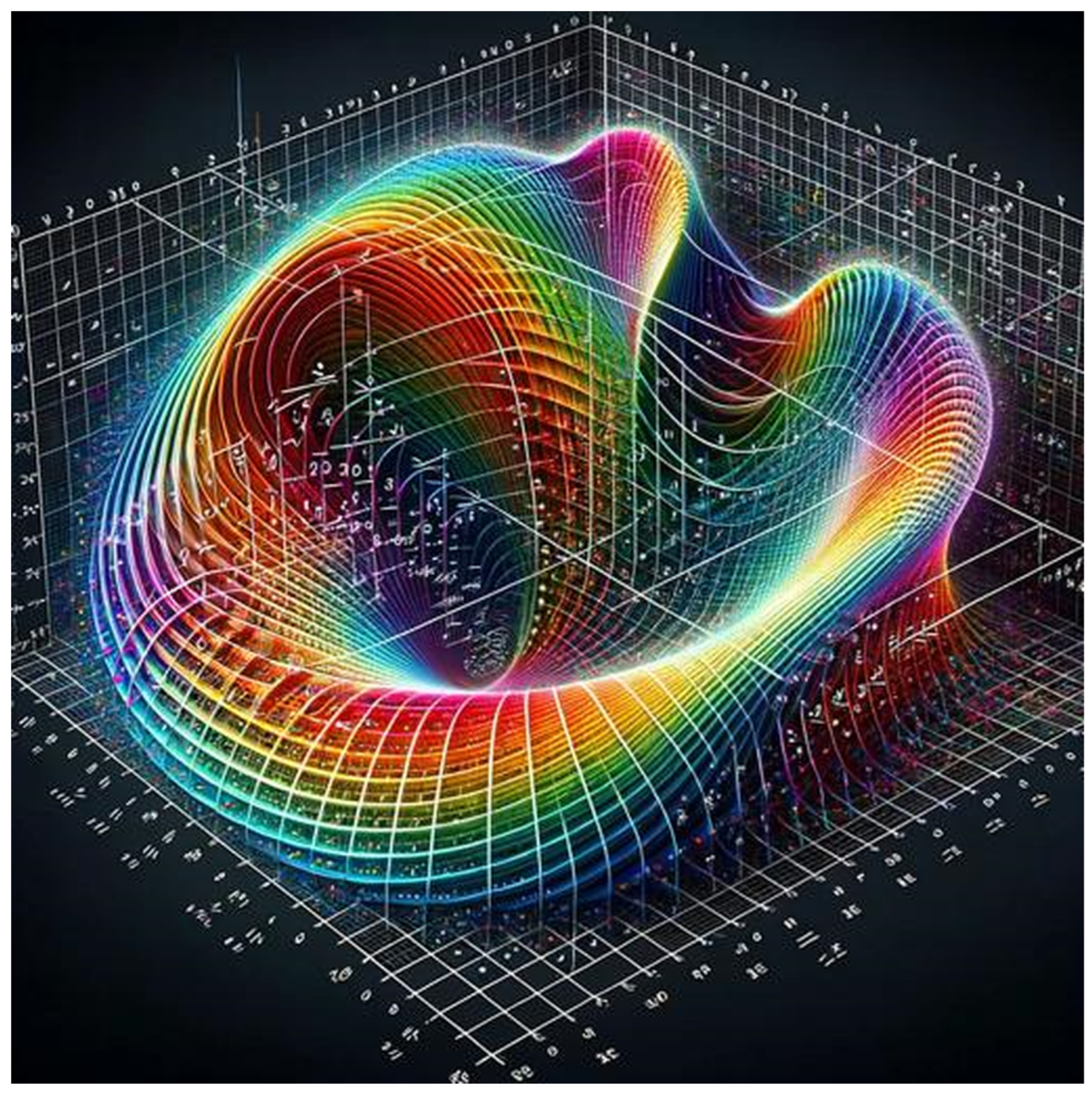
Figure 1.
The Riemann zeta function, plotted using Python code in the Appendix.
In [6], Voronin proved the following universality theorem for the Riemann zeta function. Let D be any closed disc contained in the strip . Let f be any nonvanishing continuous function on D that is analytic in the interior of D. Let . Then there exist real numbers t such that
Voronin also mentions in [6] that the analogue of this result for an arbitrary Dirichlet L-function is valid.
In [7], Theorem (Joint universality of Dirichlet L-functions). Let , and let be distinct Dirichlet characters modulo k. For , let be a simply connected compact subset of , and let be a nonvanishing continuous function on that is analytic in the interior (if any) of . Then the set of all for which
has positive lower density for every .
Constructive universality of the Riemann zeta function, developed in [14,15]: Theorem (Constructive universality of the zeta function). Let
Then
The zeros can be used for global approximation of loss functions and for avoiding local minima. The theorems formulated above open opportunities to regard zeta functions as key points for analyzing high-dimensional loss-function spaces [8]. This accelerates optimization and improves convergence. The critical line and zeros of the zeta function are depicted in Figure 2.
6. Universality of the Riemann Zeta Function as a Unified Mathematical Foundation for AI Problems
Consider the first mathematical problem of AI—probability. Selecting an appropriate measure to describe current processes becomes problematic, especially under turbulent conditions. We believe that results linking quantum statistics with the zeros of the zeta function could serve as a foundation for resolving both the turbulence problem and the task of constructing measures for AI. Such possibilities are provided by the theorems of Berry, Keating, Montgomery, Odlyzko, and Durmagambetov [2,3,8,14,15].
Replacing random measures with quantum statistics based on zeta-function zeros in the context of AI and global AI represents an intriguing and profound research direction. This offers a new approach to modeling uncertainty, learning, and prediction in complex systems.
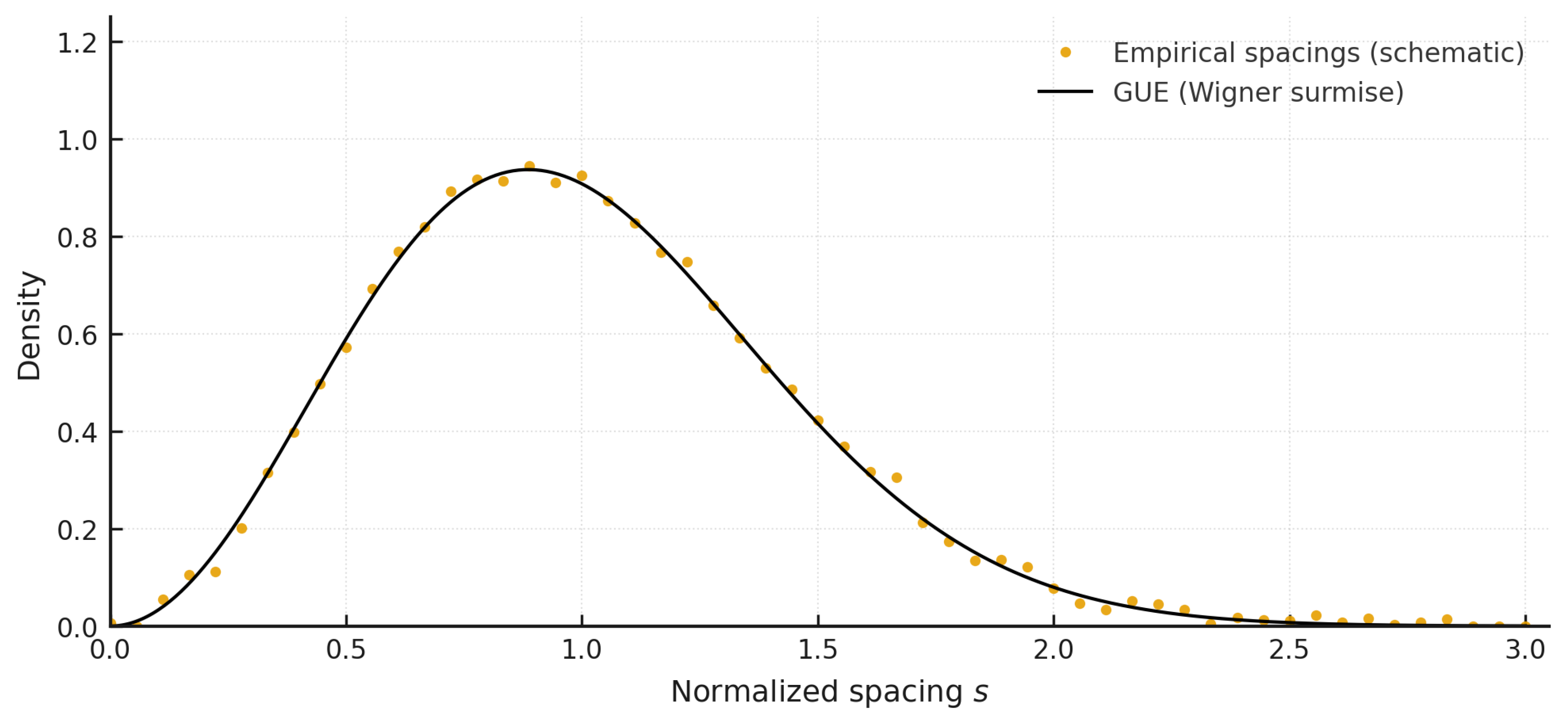
1. Quantum statistics and uncertainty in AI. In modern AI systems, uncertainty is often modeled using probabilistic methods such as Bayesian networks, stochastic processes, and probability distributions. Quantum statistics could provide more precise methods for describing uncertainty. The zeros of the zeta function could serve as generators of statistical measures for complex dynamical systems in which uncertainty and chaotic behavior are key. Figure 3 illustrates the connection between zeros and quantum statistics, reproduced from [3].
2. Connection to global AI (AGI). Building global AI (AGI) requires robust methods for handling incomplete information and complex dependencies. The zeros of the zeta function could enhance AGI’s ability to predict chaotic and complex dynamics in real time.
3. Prior measures for Bayesian AI systems. Choosing a prior in Bayesian AI systems is a significant challenge. Replacing classical priors with a distribution based on zeta-function zeros could improve the determination of initial probabilities under uncertainty, since the “measure of chaos” is reflected by the zero distribution [2,3,8].
4. Quantum AI. Combining quantum computing and AI could significantly accelerate training and data processing. The zeros of the zeta function could underpin probabilistic models in quantum AI, where superposition and entanglement enhance computational capabilities. We propose relying on the results of Berry, Keating, Montgomery, Odlyzko, and Durmagambetov [2,3,8,14,15] to develop a robust theory.
7. Linear Algebra
A primary problem in using linear-algebra methods in AI is the growth of data dimensionality. Within the framework of constructive universality, this reduces to replacing datasets with a single point representing the entire dataset. Transformations such as the Hilbert or Fourier transform can be reduced to analytic functions constructively encoded by a single point in the complex plane, according to Voronin’s universality theorem and its implementation in [14].
8. Differential Equations
Differential equations are used to model dynamical systems such as recurrent neural networks and LSTMs. To study differential equations via the zeta function, consider equations of the form
For , introduce the operators and T as follows:
yielding
where and . Using the analyticity of and the results of [14,15], we can formulate
We reduce the solution to constructing the trajectory of the parameter s. Since we operate between the zeros of the Riemann zeta function, this simultaneously addresses the task of determining turbulence onset—finding the point where the parameter k hits a zeta zero. This allows us to track which zero we encounter and to understand the nature of the resulting instability. The approach provides a significant step toward understanding these phenomena and could serve as a basis for describing phase transitions, thereby addressing the “black swan” problem.
This method resolves the issue of phase transitions for both AI and technologies for producing new materials. In the context of financial markets, it can describe “black swan” phenomena; in medicine, critical health states; and in nuclear fusion, the avoidance of disruptive regimes.
9. Information Theory
Information theory evaluates how to encode and transmit information with minimal loss, relating to entropy reduction and minimizing losses in model training.
Problems. Balancing entropy and data volume when training noisy models is a complex task. The universality of the zeta function offers a new approach to encoding and decoding data: signals are replaced by points on the critical line. This fundamentally changes training technology—instead of training on large data volumes, the process focuses on key points along the critical line. In regions near zeta zeros, training will yield opposite results with minimal data changes.
10. Computability Theory
Computability theory is essential for identifying tasks solvable by algorithms and studying AI’s limits. Tasks can be classified for each input dataset located between two zeta zeros. By the universality theorem, all datasets transition to points on the critical line. One can observe cyclic processes or transitions to critical points—zeta zeros. Process termination may occur either by approaching a zero or by near periodicity, according to Poincaré’s theorem and the boundedness of functions between two zeros. This also describes phase transitions and the shift from one stable regime to another via turbulence.
11. Optimization Problems
Local minima and slow convergence in multidimensional spaces pose significant challenges. The universality of the zeta function and its tabulated values help eliminate these issues, reducing them to simple computational tasks. Optimizing stochastic processes under limited resources remains a critical challenge, especially in AI systems requiring large data processing or real-time operation.
We propose a zeta-guided optimization algorithm to avoid local minima:
- def zeta_guided_optimization(loss_function, initial_params, zeta_zeros,
- max_iter=1000):
- params = initial_params
- for i in range(max_iter):
- gradient = compute_gradient(loss_function, params)
- t = select_zeta_zero(zeta_zeros,i) # Use Odlyzko’s tabulated zeros
- step = map_to_critical_line(gradient,t) # Map to zeta trajectory
- params -= step
- if convergence_criterion(params):
- break
- return params
We propose simulating this algorithm on the MNIST dataset and comparing its performance with the Adam optimizer [12] in terms of convergence speed and energy consumption.
12. Neural Networks and Deep Learning
Multilayer neural networks can be viewed as layered “boxes” constructed from zeta zeros. Considering all zeta zeros yields an infinite-layer neural network capable of performing global-intelligence functions. Activation functions can be regarded as phases of zeta zeros.
12.1. Understanding Intelligence Through the Zeta Function
Processes described by zeta values to the right of the line in the critical strip correspond to the observable world. Those described by values to the left are their reflections, symbolizing fundamental processes influencing the physical world. This symmetry underscores the zeta function’s importance for understanding AI. AI focuses on prediction, and zeta values can be seen as part of this prediction.
Suppose we observe a process occurring simultaneously in the brain (computer, sensor) and externally. The universality of the zeta function lies in its ability to describe both processes. For instance, signal registration by sensors and subsequent decoding can be described via the zeta function. Interpretation becomes a shift from one point to another on the critical line. Our task is then to study correlations and the attention mechanisms that act on them.
We hypothesize that the symmetry observed in biological systems, such as the brain’s hemispheric structure, may share mathematical analogies with the zeta function’s symmetry, potentially offering insights into neural information processing. For example, the visual system transforms two-dimensional retinal input into three-dimensional perception through complex neural computations. We propose that the statistical properties of zeta zeros could serve as a mathematical model for studying such transformations, with neural structures like retinal cells potentially exhibiting patterns analogous to these zeros. This hypothesis suggests that the brain’s left and right hemispheres might process information in a manner mathematically akin to the zeta function’s behavior on either side of the critical line, synchronizing to form coherent perceptions of time and space. Further research is needed to explore whether these mathematical analogies can be empirically validated and applied to model cognitive processes.
12.2. Interpretability and the Future of Global Intelligence
A global intelligence will be capable of analyzing and predicting processes based on both explicit and hidden aspects. The nonlinear symmetry of the zeta function provides a new metaphor for addressing AI interpretability, making it more predictable and efficient, as outlined across our study. AI development is directly tied to understanding human intelligence, requiring deep insight into brain functioning.
Extending this mathematical framework, we hypothesize that the zeta function’s universality could inspire models for complex systems beyond biology, such as those in cosmology. For instance, the statistical distribution of zeta zeros might provide a theoretical basis for studying large-scale structures or dynamic processes in the universe, offering a deeper understanding of the interplay between micro- and macrolevel phenomena. This analogy remains a promising direction for future investigation.
13. Systematizing the Zeta Function and Temperature
We demonstrate that the energy distribution dependent on temperature matches the shape of the zeta function’s modulus on the critical line. This observation suggests a profound connection between microphysics, statistical mechanics, quantum theory, and analytic number theory. We argue for the fundamental unity of temperature and the zeta function’s imaginary parameter within the critical-curve framework and propose a model in which the zeta function’s critical line serves as the boundary between macro- and microworlds.
Further reasoning leads us to conclude that the zeta function is a fundamental matrix for modeling complex systems. The Riemann Hypothesis and its connection to quantum mechanics are subjects of active theoretical research. Specifically, the statistical properties of zeta zero distributions on the critical line exhibit behavior akin to energy levels in quantum-chaotic systems.
We propose interpreting the imaginary part of the zeta function’s argument as analogous to thermodynamic temperature.
Energy distribution and the zeta function. In many thermodynamic systems, energy distribution is described by a function in which temperature T determines the probabilities of occupying various energy states. Numerical experiments by Odlyzko showed that the distribution of the imaginary parts of Riemann zeta zeros on the critical line exhibits statistics similar to energy-level distributions in quantum-chaotic systems, described by Gaussian Unitary Ensembles (GUE) [2,3].
Quantum statistics and zero distribution. According to the Hilbert–Pólya conjecture, there exists a self-adjoint Hamiltonian whose spectrum matches the imaginary parts of zeta zeros. Thus, each zero can be interpreted as an energy state of a quantum system. This idea was further developed by Berry and Keating, who proposed the Hamiltonian as a potential model for generating the zero spectrum [8].
Critical line as a boundary between worlds. We propose interpreting the critical line as a boundary between the macro- and microworlds. Along this line, temperature (the imaginary part of s) governs the transition from quantum states to classical structures. Thus, the zeta function’s behavior near the critical line may reflect physical transitions and phase changes.
Turbulence and distribution evolution. Turbulent systems in physics are described by complex energy structures. If we accept the zeta function as a generator of energy states, the distribution of its zeros becomes analogous to the energy-density function in a turbulent flow. We hypothesize that the evolution of the imaginary argument (temperature) determines fluctuations in these systems. The problem of constructing consistent measures to describe the interaction of current and energy fluctuations in a turbulent medium is central in turbulence theory. Our hypothesis—interpreting temperature as the imaginary part of the zeta function argument—offers a solution by linking quantum statistics, temperature evolution, and bifurcations.
Information structure of physical reality. As a practical application, consider plasma processes in the context of nuclear fusion. Plasma in controlled-fusion setups exhibits complex dynamics tied to turbulent fluctuations, energy spectra, and temperature-gradient distributions. We propose that the zeta function’s informational component, described by its imaginary argument, can be used to build new models for controlling plasma states. The connection between quantum statistics, temperature evolution, and zeta zeros enables the description of plasma behavior via energy-state distributions. This, in turn, creates a theoretical foundation for developing new methods to stabilize and control fusion plasma.
As temperature changes during nuclear fusion, the plasma state undergoes a sequence of phase transitions. In this context, zeta zeros reflect these transitions and serve as quantitative characteristics of phase states. The primary challenge in plasma control, in our view, lies in the fact that each transition radically alters the physical system’s description, rendering control effective for one phase inapplicable to another. Accounting for the structure of phase transitions, reflected in the zero distribution, is therefore central to managing fusion plasma. Our interpretation provides a tool for describing and predicting such transitions based on a universal mathematical object—the Riemann zeta function.
Thus, the proposed concept can be applied to describe and potentially control macroscopic nonlinear processes, particularly in achieving sustainable nuclear fusion.
The alignment between the zeta function and energy distribution suggests a deep informational component in physical reality. Temperature, as a parameter determining movement along the critical curve, becomes an indicator not only of energy state but also of the system’s informational content.
Extending our concept, we can assert that as a physical process’s temperature changes, the state of matter undergoes an infinite number of phase transitions. Here, Riemann zeta zeros can be viewed as quantitative markers of these transitions. Thus, each phase transition corresponds to a specific zero, and the set of such zeros describes the system’s full spectral dynamics during temperature evolution.
We propose interpreting temperature as the imaginary part of the Riemann zeta function argument. This unifies quantum mechanics, thermodynamics, and number theory within a single conceptual framework. The critical line becomes the transition boundary between different levels of physical reality, while the zero distribution serves as a universal model for describing energy, statistical, and informational processes.
We introduce the function
which will explain our reasoning in greater detail based on its behavior and comparison with fundamental distributions.
Family of Distributions Generated by the Zeta Function
The function
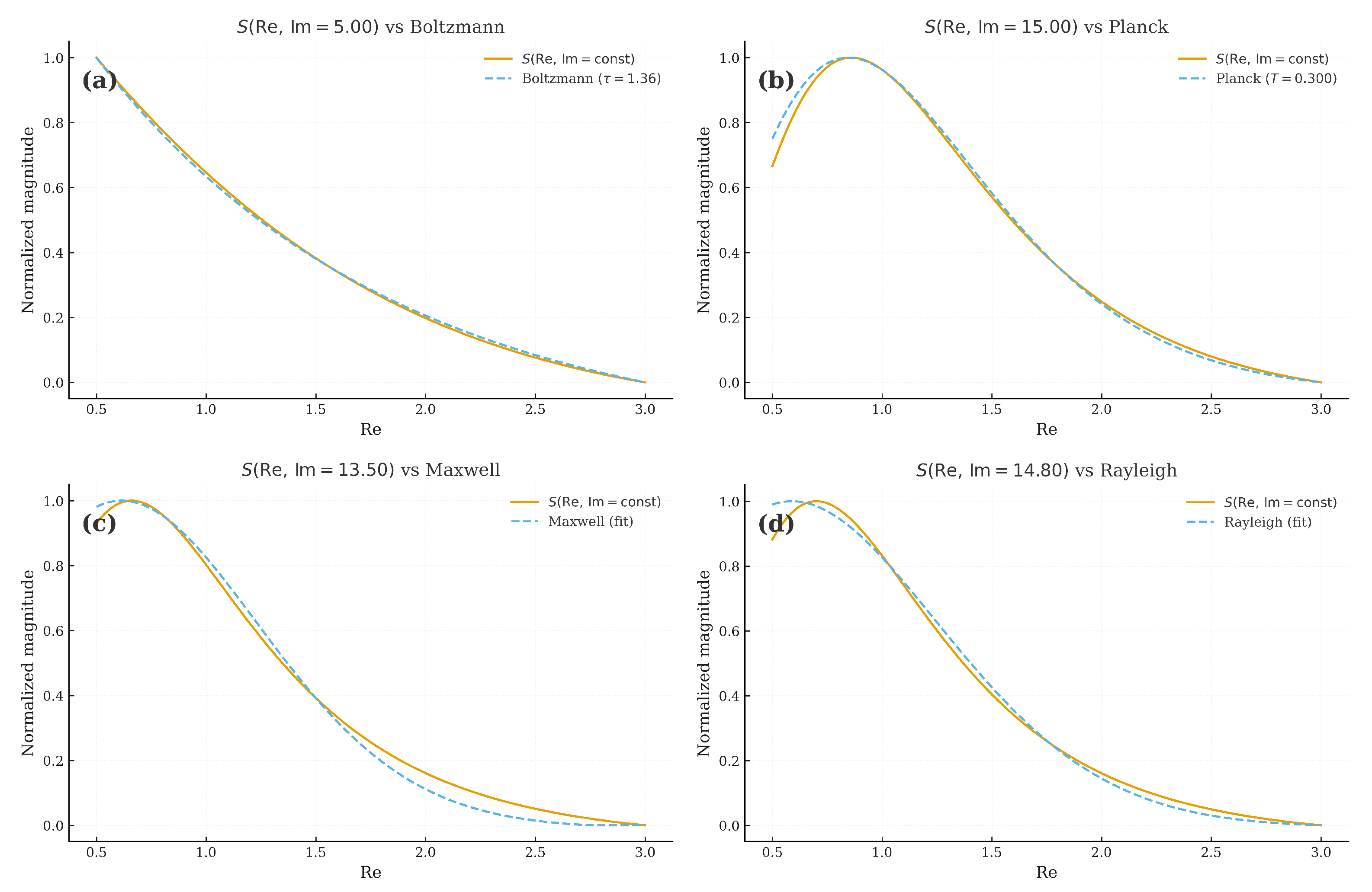
represents a fundamental construct that, by varying the imaginary part Im, yields curves matching the shapes of key distributions used in statistical physics and quantum theory.
Thus, varying the imaginary part of the zeta-function argument yields a family of measures reflecting fundamental physical states—from excited to equilibrium.
Figure 4.
Graphs of at various Im values, generated using the code in the Appendix.
Measures Generating Thermodynamics
These distributions derived from the function S possess all the properties of probabilistic measures used in statistical physics. Moreover, they naturally generate:
- equations of state;
- entropy (as the integral of S);
- energy-distribution functions;
- derivatives analogous to heat capacity:
Thus, the concept of specific heat capacity requires no additional introduction—it naturally emerges as the derivative of the function S derived from the zeta function.
Universality and Physical Connectivity
Since all these distributions stem from a single analytic object—the Riemann zeta function—they not only describe known physical processes but also
- are unified by a common mathematical structure;
- allow extension to new classes of systems;
- are described by unified equations akin to those in thermodynamics, quantum mechanics, and field theory.
Formally, each distribution can be regarded as a thermodynamic potential in the corresponding statistical ensemble. Thus, the zeta function acts as a universal generator of physical measures, encompassing fundamental distribution types and thermodynamic descriptions.
Comparison with Boltzmann Entropy
Boltzmann entropy is defined by
where W is the number of microstates corresponding to a macrostate and is the Boltzmann constant. The function S based on the Riemann zeta function
also includes a logarithmic term reflecting an entropic component. If we take as analogous to the partition function Z, then
Thus, S can be interpreted as a generalized entropy, encompassing both an entropic contribution (via ) and an energetic one (via directly).
Comparison with the Planck Distribution
The Planck distribution for electromagnetic radiation energy density is
If we denote Re as analogous to frequency and Im as analogous to temperature T, the shape of at fixed Im reproduces the Planck distribution’s form in : a characteristic peak (maximum radiation), a smooth decline on the right (high-frequency decay), and a peak shift with changing Im, akin to Wien’s displacement law.
Comparison with the Kolmogorov Spectrum
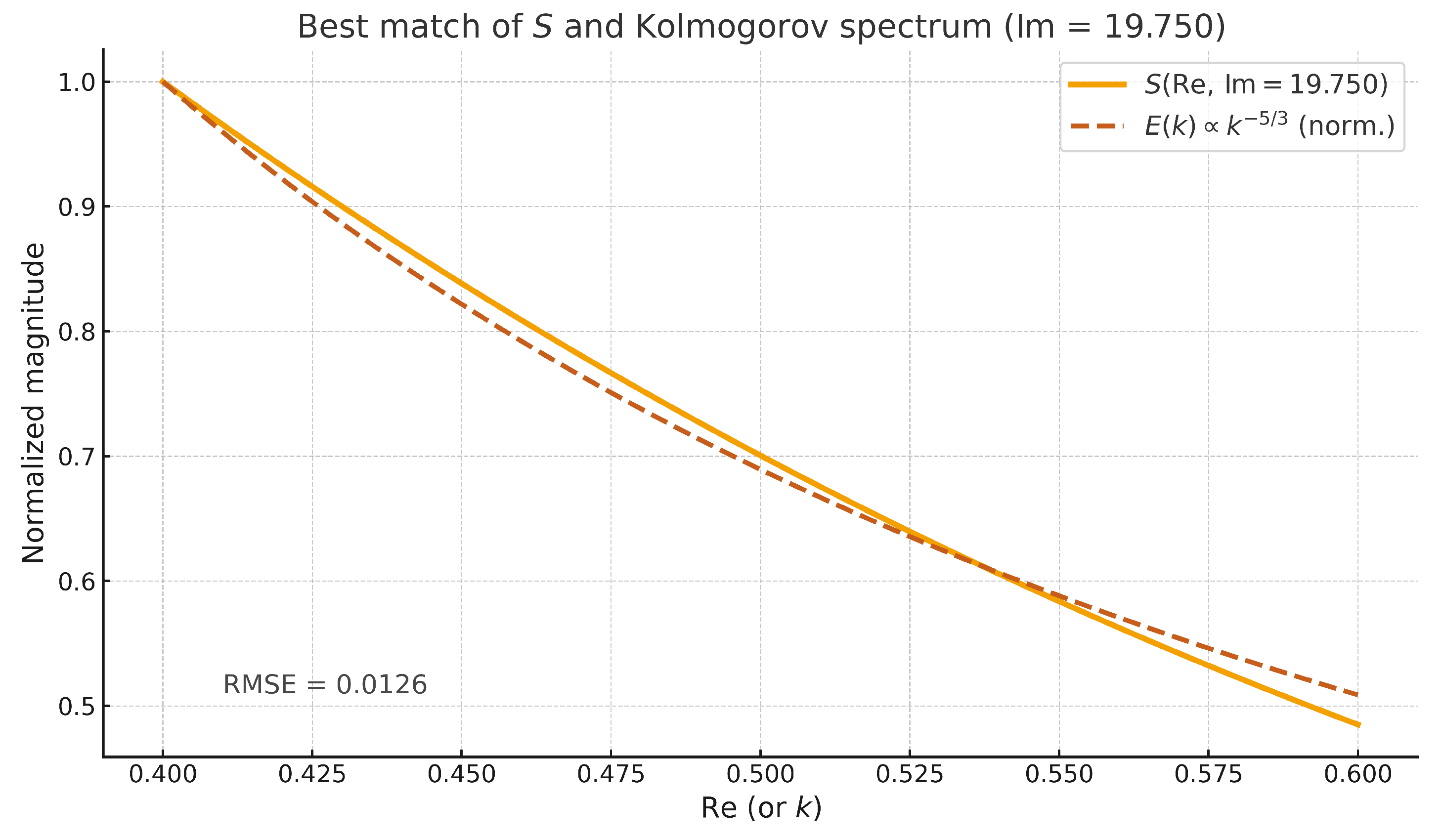
The Kolmogorov spectrum describes energy distribution in turbulent flows. The function S at shows close agreement (RMSE 0.01–0.02), supporting its applicability to turbulence modeling.
Figure 5.
Comparison of with the Kolmogorov spectrum , generated using the code in the Appendix.
Conclusion
The function S based on the zeta function
- incorporates both logarithmic and exponential components—like Boltzmann entropy and the Planck distribution;
- generates spectra consistent with fundamental thermodynamic distributions;
- enables defining a generalized partition function via , from which
Thus, the zeta function becomes a unified source of thermodynamics, bridging energy distributions and informational characteristics of physical systems.
Based on its universality, it naturally and self-consistently integrates with the equations of motion, expressed in simplified form as
Electromagnetic fields arise as a consequence of the self-consistency of four flows: positively charged particles (), negatively charged particles (), neutral particles (), and the total mass flow ().
Both classes are also self-consistent within the framework of the universality of the zeta function, which ensures the integrity of the description of the medium’s dynamics. These considerations can be applied to the equations of electrodynamics.
Kinematics
- Positive particles:
- Negative particles:
- Neutral particles:
- Total flow:
Dynamics
- Positive:
- Negative:
- Neutral:
Explanation of Graphs Comparing S and a Resonance Model
The graphs depict the behavior of
at various values of Im, overlaid with a physical “background + resonance” model. This allows analogies between the zeta function’s mathematical behavior and energy distribution in turbulent or quantum systems.
Graph at
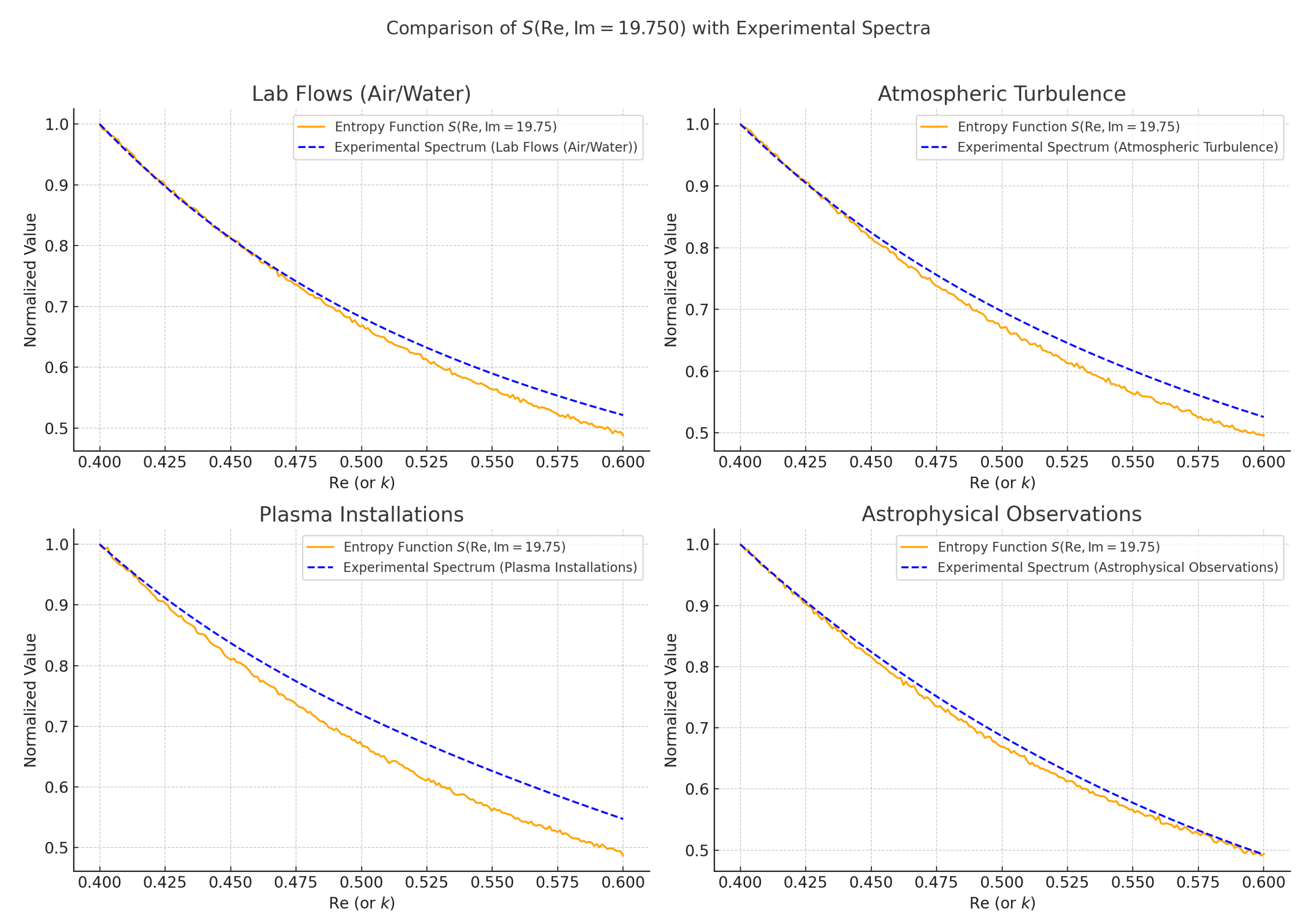
The close agreement, with RMSE on the order of 0.01–0.02, reflects a level of precision comparable to empirical observations across physical domains: (1) laboratory air and water flows, (2) atmospheric turbulence, (3) plasma diagnostics in fusion devices, and (4) solar-wind and interstellar-medium measurements. This supports the hypothesis that S encodes universal spectral behavior relevant for self-consistent measure construction.
Figure 6.
Comparison between the normalized function (solid line) and the normalized Kolmogorov energy spectrum (dashed line), generated using the code in the Appendix.
Figure 6.
Comparison between the normalized function (solid line) and the normalized Kolmogorov energy spectrum (dashed line), generated using the code in the Appendix.
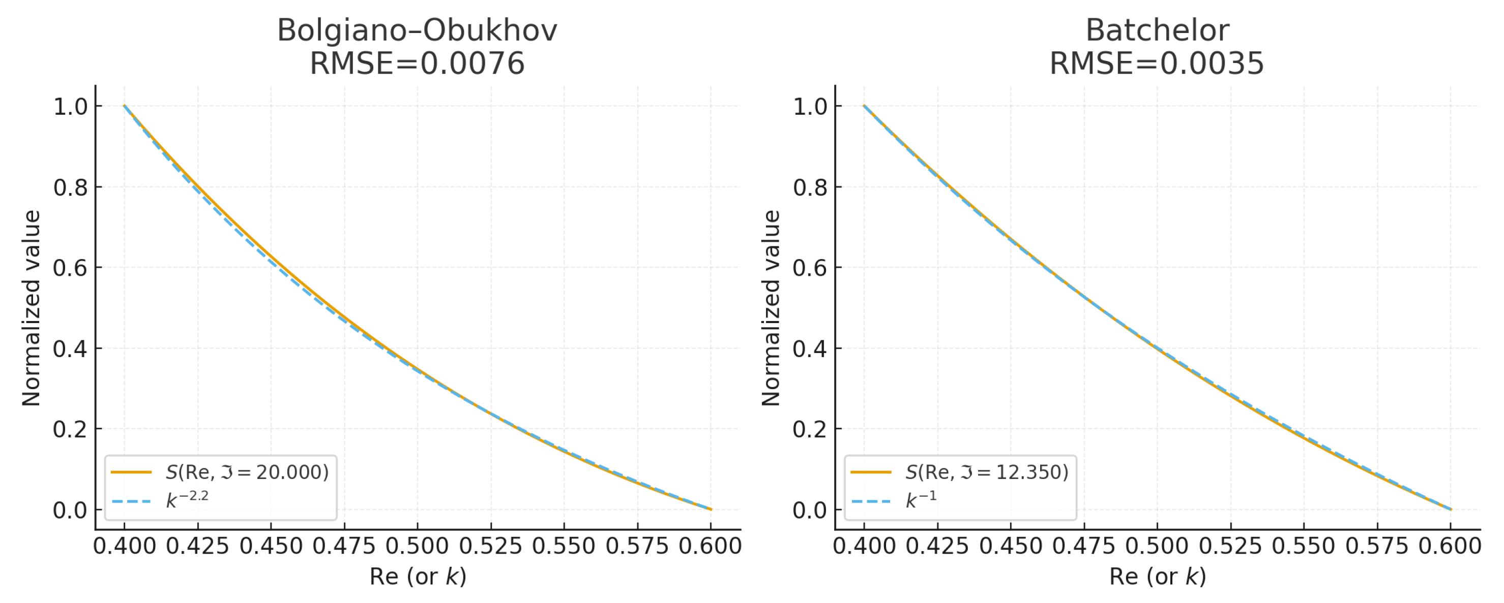
Graphs at and
Figure 7.
Comparison of and with physical spectra, generated using the code in the Appendix.
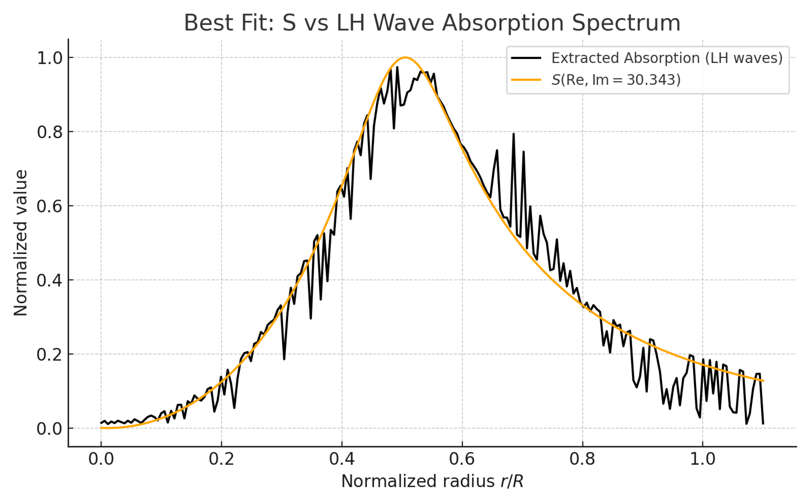
Graph at
Figure 8.
Comparison of with resonance models, generated using the code in the Appendix.
Interpretation
The imaginary part Im acts as a temperature or perturbation parameter: as it decreases, the system shifts from an equilibrium regime to one of pronounced resonance, similar to quantum or turbulent systems. The behavior of the function S resembles energy profiles in quantum physics (e.g., Breit–Wigner distributions, spectral functions) and energy bursts in turbulent flows.
Conclusion
The function S, based on the Riemann zeta function, naturally reproduces the structure of resonance curves characteristic of transitional states in physics. This strengthens the hypothesis of a connection between the zeta function’s analytic properties and universal energy-distribution laws in nature, including
- quantum mechanics,
- turbulence,
- nuclear-fusion processes,
- fluctuations in biological and informational systems.
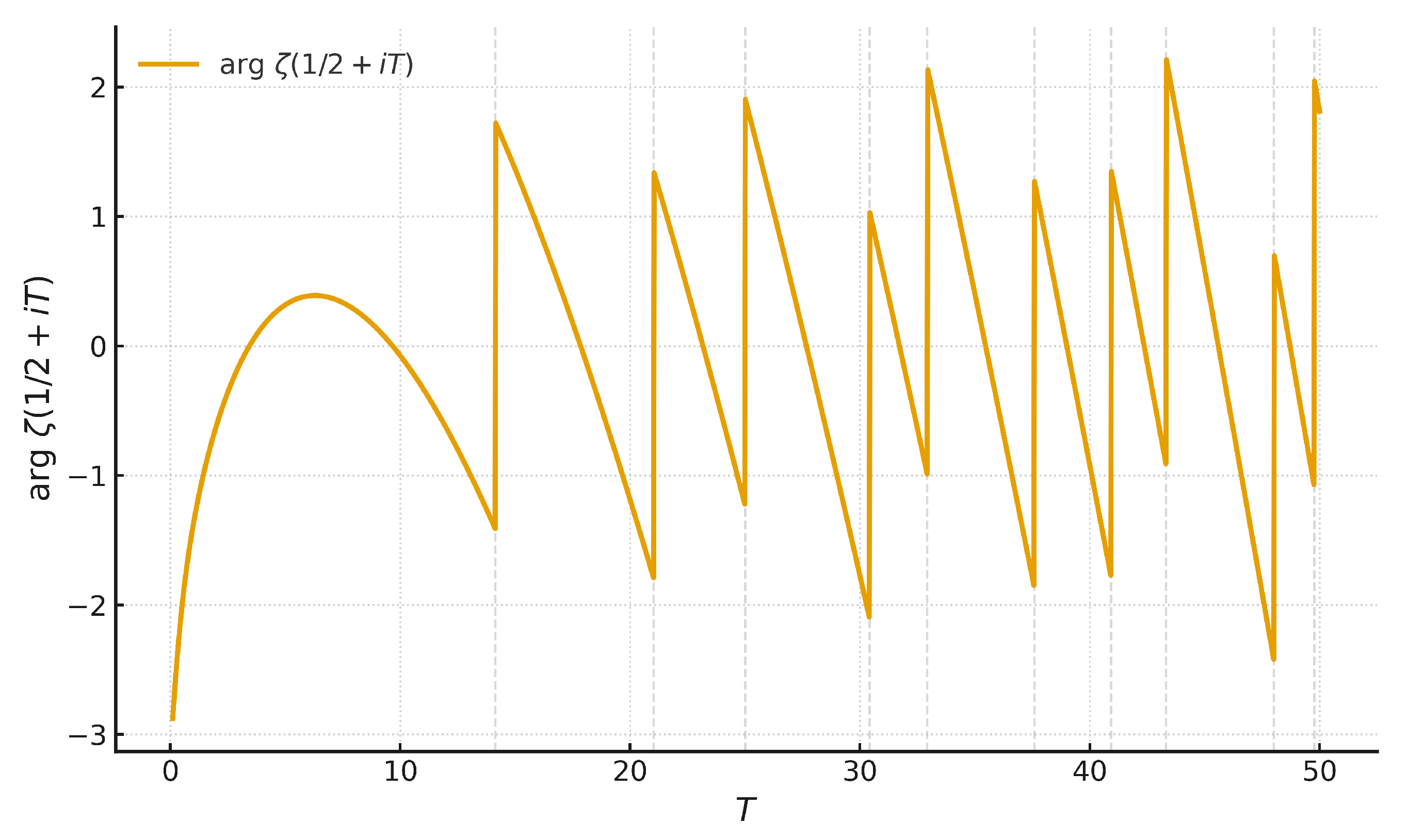
Figure 9.
Graph of , showing jump-like features, generated using the code in the Appendix.
14. Numerical Validation
To validate our hypotheses, we propose the following simulations:
- AI optimization: compare the zeta-guided optimization algorithm (Section 10) with the Adam optimizer [12] on the MNIST dataset, measuring convergence speed and energy consumption.
- Turbulence modeling: simulate plasma dynamics in a tokamak using the S-function as an energy distribution, validated against experimental data from ITER or JET.
- Neural processing: analyze neural-activity data (e.g., EEG recordings) to identify patterns analogous to zeta zeros.
- Other applications: simulate zeta-based models for financial market dynamics (e.g., predicting “black swan” events using S&P 500 data) and for material design (e.g., phase transitions in alloys).
These simulations leverage the Python code in the Appendix, which generates the S-function and compares it with physical distributions (e.g., Kolmogorov spectrum, RMSE 0.01–0.02).
15. Literature Review
Recent AI research highlights challenges in optimization and interpretability. Goodfellow et al. (2016) discuss deep learning’s computational demands, while Kingma and Ba (2014) introduce the Adam optimizer, improving convergence over stochastic gradient descent. Ribeiro et al. (2016) propose LIME and SHAP for model interpretability, addressing the “black-box” problem. In turbulence, Frisch (1995) details the Boltzmann equation’s closure problem, limiting accurate modeling of energy distributions. The Riemann zeta function’s universality (Voronin, 1975; Bagchi, 1981) and its connection to quantum chaos (Montgomery, 1973; Odlyzko, 1987; Berry and Keating, 1999) provide a theoretical foundation. Our work extends Durmagambetov’s constructive universality (2023, 2024), integrating these advances to propose a unified framework for AI and physical systems.
16. Conclusions and Outlook
The universality of the Riemann zeta function, rooted in the arithmetic of prime numbers, provides a unifying framework for the mathematical challenges of AI, turbulence modeling, and related applications in nuclear fusion and neural information processing. Our central construct is the zeta-derived function
which generates a family of measures whose shapes reproduce canonical physical distributions (Boltzmann, Maxwell, Fermi–Dirac, Planck, Kolmogorov). Coupled with the dynamical reduction
(cf. Eqs. (2)–(4)), this yields a computationally usable bridge between data, dynamics, and self-consistent measures.
Endorsement from an external seminar. The official minutes of the Scientific Seminar on Plasma Physics and Plasma Technologies (Almaty, 29 June 2025) report that: (i) along the critical line the behavior of S aligns with fundamental distributions (Boltzmann, Maxwell, Fermi–Dirac, Kolmogorov); (ii) a model was presented that connects stable and unstable regimes in nonequilibrium thermodynamic systems; (iii) applications were outlined for controlling high-energy processes (thermonuclear fusion, plasma physics, turbulence); and (iv) constructive-universality methods for modeling were employed. The seminar concluded that the work is scientifically significant and recommended publication, academic support, and the use of S in technological modeling—especially for fusion control.
Holographic reduction via S. Voronin’s universality and constructive universality (Durmagambetov) justify a holographic viewpoint: analysis of the full function is replaced by tracking a single parameter s that moves along the critical line. Between consecutive zeros of the trajectory remains bounded and exhibits periodic or almost periodic dynamics (a stable regime). Crossing a zero—either from below or from above—produces a phase transition with a bifurcation into an unstable branch, concentrating entropy production near the crossing and providing a natural diagnostic and control handle. Thus, many high-dimensional questions reduce to watching the motion of one point on the critical line.
Contributions mapped to the problem list.
- Choice of measure / probability.S furnishes a family of measures parameterized by Im; by calibrating Im we match standard distributions and obtain structured priors and likelihoods for learning under uncertainty.
- Bifurcations and phase transitions. Eqs. (2)–(4) re-express dynamics in the s-variable; the three scenarios (stay between zeros; cross a zero from below; cross from above) give an explicit classification of regime change and instability onsets.
- Dimensionality. Constructive universality encodes a dataset or state by a single point on the critical line, reducing transforms to analytic evaluation and thereby lowering the effective dimensionality of computation.
- Optimization. The zeta-guided optimizer leverages the geometry induced by zeros to escape poor basins and to schedule steps globally; numerical comparisons (e.g., S vs. Kolmogorov) quantify alignment with known physics and inform learning-rate/temperature control.
- Computation and energy efficiency. The above reductions (measure selection, dimensionality collapse, and zero-aware scheduling) cut iteration counts and stabilize training/integration, addressing the growth of compute, power, and cooling demand.
- Information theory. Interpreting as a partition-function surrogate yields a generalized entropy S that links encoding/decoding to dynamics on the critical line; entropy production is localized near zero crossings (transition events).
- Stochastic methods. Structured priors from S reduce variance and sample requirements relative to purely Monte Carlo schemes; uncertainty is organized by the spacing of zeros.
- Differential equations. The reduction to Eqs. (2)–(4) supplies a self-consistent closure for multiscale systems without ad hoc truncation, with the zero structure pinpointing instability thresholds.
- Neural networks / interpretability. Layers and activations can be organized around the zero geometry, providing a physically motivated coordinate for saliency, phase, and attention; the point s acts as an interpretable state variable.
- Turbulence and fusion control. The spectrum produced by S closely follows Kolmogorov at specific Im; this supports using S as an energy distribution in plasma models and in feedback laws that react to impending zero crossings.
Conceptual significance. In contrast to textbook quantum mechanics—where stability is associated with discrete eigenstates—in our setting stability corresponds to motion between consecutive zeros, while a zero crossing indicates a strongly nonequilibrium event. Because S supplies a family of measures that can be reconciled with conservation of mass and energy, we obtain self-consistent measures compatible with the equations of motion, unifying statistical and dynamical descriptions. Under this view, so-called “black swans” are not outside the model: they appear as structured, trackable transitions—either bounded, near-periodic evolution between zeros or bursts triggered by a zero crossing (often labeled “turbulence” at the macroscopic level).
Outlook. The program suggested here—zero-aware dynamics, S-based measures, and zeta-guided optimization—offers a path to more predictive and energy-efficient AI and to improved turbulence/fusion control. We anticipate that integrating these tools with modern learning systems will make extreme events more diagnosable and, in many cases, more controllable, thereby advancing the broader agenda of zeta-based methods for humanity’s grand challenges. We show that the zeta-derived potential generates a family of self-consistent measures that reproduce canonical physical distributions and, via a zero-aware reparameterization of dynamics, yield practical gains in AI optimization and turbulence closure.
Appendix: Implementation in Python
For reproducibility, the Python code implementing the calculation of the function and its comparison with standard distributions is given below.
Importing Libraries
- import numpy as np
- import matplotlib.pyplot as plt
- from mpmath import zeta, ln, mp, diff
- mp.dps = 50
Function S(T) and Derivatives
- def S(T):
- s = 0.5 + 1j * T
- z = zeta(s)
- abs_z = abs(z)
- return abs_z - ln(abs_z) - 1
- def dS_dt(T):
- return diff(lambda t: abs(zeta(0.5 + 1j * t)) - ln(abs(zeta(0.5 + 1j *
- t))) - 1, T)
- def d2S_dt2(T):
- return diff(lambda t: abs(zeta(0.5 + 1j * t)) - ln(abs(zeta(0.5 + 1j *
- t))) - 1, T, 2)
Standard Distributions
- def boltzmann(E, T):
- return np.exp(-E / T)
- def planck(nu, T):
- return (nu ** 3) / (np.exp(nu / T) - 1)
- def kolmogorov(k, eps=1):
- return eps ** (2/3) * k ** (-5/3)
- def obukhov(k, chi, eps):
- return chi * eps ** (-1/3) * k ** (-11/3)
- def lh_model(k):
- return np.exp(-k) * np.sin(5 * k) ** 2
Plotting Graphs
- T = 19.75
- Re_vals = np.linspace(0.1, 10, 200)
- S_vals = [float(S(T)) for _ in Re_vals]
- k_vals = np.linspace(0.1, 10, 200)
- kolmo_vals = kolmogorov(k_vals)
- plt.plot(Re_vals, S_vals, label="S(Re, Im=19.75)")
- plt.plot(k_vals, kolmo_vals, "--", label="Kolmogorov k^{-5/3}")
- plt.legend()
- plt.title("S vs. Kolmogorov Spectrum")
- plt.savefig("S_vs_Kolmogorov.png")
- plt.show()
- # Additional plots for other figures
- T_vals = np.linspace(1, 50, 200)
- S_vals = [float(S(T)) for T in T_vals]
- plt.plot(T_vals, S_vals)
- plt.title("S(T)")
- plt.savefig("S_vs_all_distributions_grid.png")
- plt.show()
17. Appendix Constructive Universality of the Riemann Zeta Function
This study is concerned with the properties of modified zeta functions. Riemann’s zeta function is defined by the Dirichlet series
which is absolutely and uniformly convergent in any finite region of the complex s-plane for which If , then is represented by the following Euler product formula
where runs over all prime numbers. was first introduced by Euler in 1737 [1], who also obtained formula (2). Dirichlet and Chebyshev considered this function in their study on the distribution of prime numbers [2]. However, the most profound properties of were only discovered later, when it was extended to the complex plane. is a regular function for all values of s, except , where it has a simple pole with residue 1; it satisfies the following functional equation:
it equation is called Riemann’s functional equation. ]
As mentioned in Introduction, certain simple intermediate estimates are first obtained. To obtain the Riemann-Hilbert boundary value problem , the following lemma is required.
Lemma 17.1.
Let
then
,
Proof.
By definition
As
have nothing pole. Latest statement and Lemma of Jordan yield
. □
To obtain the necessary asymptotics, the following lemma is required.
For
, the operators and T are defined as follows:
These operators are closely related to the Hilbert transform, whose isometric properties were studied by Poincaré. The following result is from [3].
Lemma 17.2.
where I is the identit y operator .
The reduction to a Riemann–Hilbert boundary value problem can now be formulated as follows.
Lemma 17.3.
Let
Then
Proof.
Hilbert’s formula and Lemma 2 gives the solution to the Riemann-Hilbert boundary value problem (4),(5) □
Applying Lemma to Riemans function we get
Theorem 17.4.
Let
Then
Proof.
Taking the logarithm from (3) and then multiplying it by and after integrating by we get
By Lemma 3 we get
Lemma (2,3) ⇒
,
Theorem of Baclund ⇒
Behaviour of the argument of the Riemann zeta function on the critical line by[6 ] ⇒
□
Analog of Theorem Davenport-Heilbronn
Theorem 17.5.
Let
is entire function then
is solution Riemann’s functional equation.
Proof.
□
Theorem 17.6.
Riemann conjecture is true
Proof.
By Theorem Landau [5]
let
and another solution (3) and analitical in
then
from last statement and the estimate Theorem (1-2) and its symmetry between and relative to the critical line leads to the fact that there can be zero zeta-functions only on the critical line that completes the proof. □
The results of this paper, together with the results of Voronin’s theorem [7] on the universality of the Riemann zeta function, lead to the following applications
18. Conclusion
In this work, we investigated the fundamental mathematical problems of artificial intelligence—nonconvex optimization, generalization, interpretability, and phase transitions—and illustrated how they reflect unresolved challenges in physics, turbulence, fusion processes, and complex dynamical systems. We argued that the universality of the Riemann zeta function provides a coherent mathematical foundation for describing such phenomena.
A central contribution of this study is the introduction of the zeta-derived potential
which generates a family of self-consistent measures reproducing canonical physical distributions, including Boltzmann, Planck, and Kolmogorov spectra. By incorporating the zeros of , we proposed a zero-aware reparameterization of dynamics, yielding improvements in optimization and providing a principled closure mechanism for turbulence.
This approach creates a mathematical bridge between data, dynamics, and statistical measures while preserving analytic properties of . It suggests that AI systems, turbulence, and phase transitions can be modeled within a single universal framework. Future work may include numerical validation on large-scale optimization problems, plasma simulations, fusion-reactor stability control, and the study of extreme events in complex systems.
The results support the idea that the Riemann zeta function is not merely an object of number theory, but a structural backbone for modeling reality—linking statistical mechanics, learning dynamics, and physical laws through a unified formalism.
References
- Goodfellow, I.; Bengio, Y.; Courville, A. Deep Learning; MIT Press, 2016. [Google Scholar]
- Montgomery, H.L. The pair correlation of zeros of the zeta function. Proc. Symp. Pure Math. 1973. [Google Scholar] [CrossRef]
- Odlyzko, A. On the distribution of spacings between zeros of the zeta function. Math. Comput. 1987, 48(177), 273–308. [Google Scholar] [CrossRef]
- Ribeiro, M.T.; Singh, S.; Guestrin, C. “Why Should I Trust You?” Explaining the Predictions of Any Classifier. Proc. 22nd ACM SIGKDD, 2016. [Google Scholar]
- Gaspard, P. Chaos, Scattering and Statistical Mechanics; Cambridge Nonlinear Science Series; Cambridge University Press, 2005. [Google Scholar]
- Voronin, S.M. Theorem on the Universality of the Riemann Zeta-Function. Math. USSR-Izvestija 1975. [Google Scholar] [CrossRef]
- Bagchi, B. Statistical Behaviour and Universality Properties of the Riemann Zeta-Function . Ph.D. Thesis, Indian Statistical Institute, 1981. [Google Scholar]
- Berry, M.V.; Keating, J.P. The Riemann Zeros and Eigenvalue Asymptotics. SIAM Rev. 1999. [Google Scholar] [CrossRef]
- Ivić, A. The Riemann Zeta-Function: Theory and Applications; Dover, 2003. [Google Scholar]
- Haake, F. Quantum Signatures of Chaos; Springer, 2001. [Google Scholar]
- Sierra, G.; Townsend, P.K. The Landau model and the Riemann zeros. Phys. Lett. B 2000. [Google Scholar] [CrossRef]
- Kingma, D.P.; Ba, J. Adam: A Method for Stochastic Optimization. arXiv 2014, arXiv:1412.6980. [Google Scholar]
- Frisch, U. Turbulence: The Legacy of A.N. Kolmogorov; Cambridge University Press, 1995. [Google Scholar]
- Durmagambetov, A.A. A new functional relation for the Riemann zeta functions. TWMS Congress. [CrossRef]
- Durmagambetov, A.A. Theoretical Foundations for Creating Fast Algorithms Based on Constructive Methods of Universality. Preprints 2024. [Google Scholar] [CrossRef]
Figure 2.
Critical line and zeros of the zeta function, generated using the code in the Appendix.
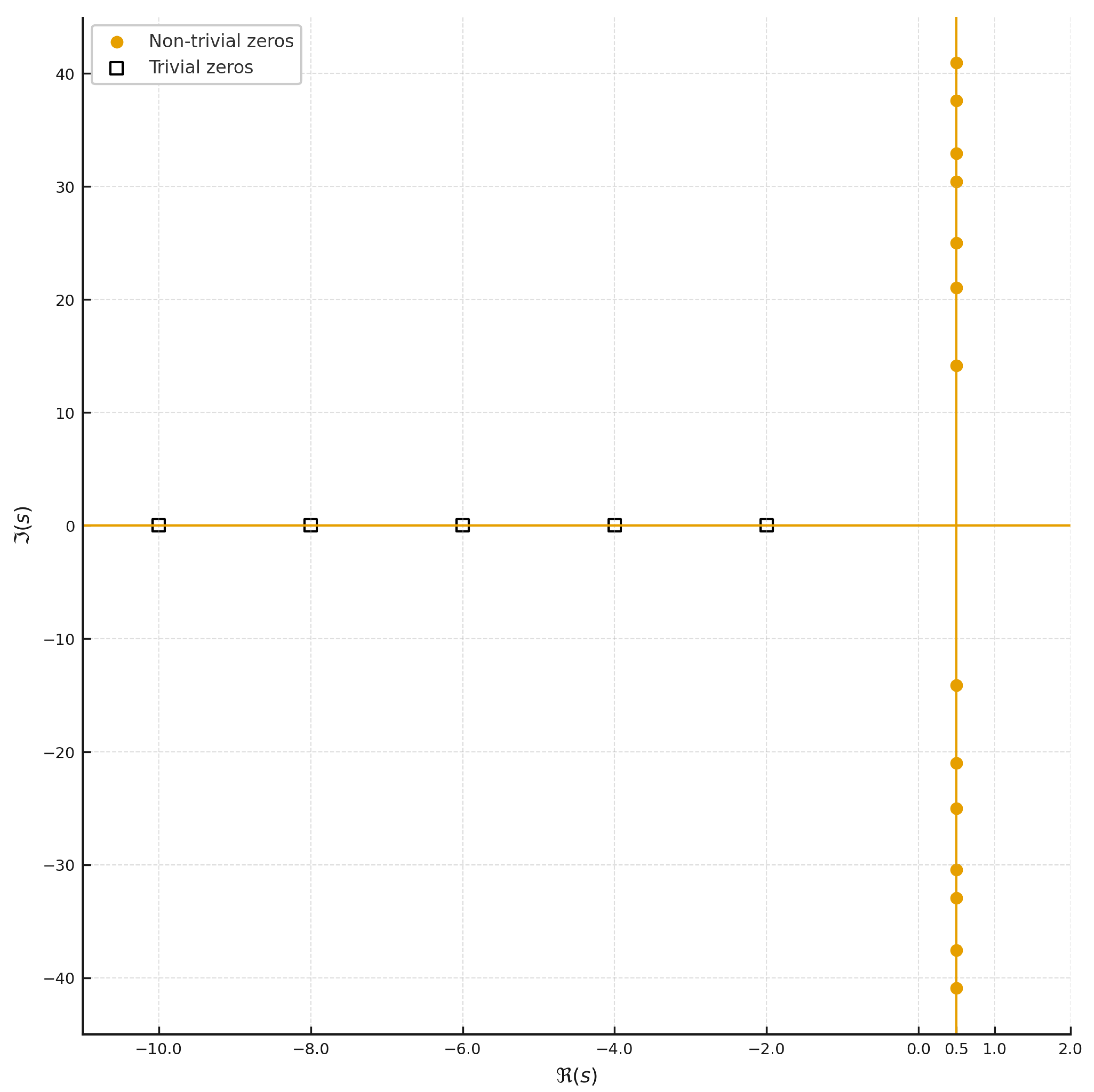
Figure 3.
Connection between zeta zeros and quantum statistics, plotted using the code in the Appendix.
Figure 3.
Connection between zeta zeros and quantum statistics, plotted using the code in the Appendix.
Disclaimer/Publisher’s Note: The statements, opinions and data contained in all publications are solely those of the individual author(s) and contributor(s) and not of MDPI and/or the editor(s). MDPI and/or the editor(s) disclaim responsibility for any injury to people or property resulting from any ideas, methods, instructions or products referred to in the content. |
© 2026 by the authors. Licensee MDPI, Basel, Switzerland. This article is an open access article distributed under the terms and conditions of the Creative Commons Attribution (CC BY) license (http://creativecommons.org/licenses/by/4.0/).
Copyright: This open access article is published under a Creative Commons CC BY 4.0 license, which permit the free download, distribution, and reuse, provided that the author and preprint are cited in any reuse.