Submitted:
24 September 2024
Posted:
25 September 2024
You are already at the latest version
Abstract
As sequencing technologies advance, short DNA sequence fragments increasingly serve as DNA barcodes for species identification. Rapid acquisition of DNA sequences from diverse organisms is now possible, highlighting the increasing significance of DNA sequence analysis tools in species identification. This study introduces a new approach for species classification with DNA barcodes based on an ensemble of deep neural networks (DNN). Several techniques are proposed and empirically evaluated for converting raw DNA sequence data into images fed into the DNNs. The best-performing approach is obtained by representing each pair of DNA bases with the value of a related physicochemical property. By utilizing different physicochemical properties, we can create an ensemble of networks. Our proposed ensemble obtains state-of-the-art performance on both simulated and real data sets. The code of the proposed approach is available at https://github.com/LorisNanni/AI-powered-Biodiversity-Assessment-Species-Classification-via-DNA-Barcoding-and-Deep-Learning .
Keywords:
DNA barcoding
; ensemble
; convolutional neural networks
1. Introduction
The current scientific consensus estimates the existence of approximately 8.7 million species on Earth, yet a mere 1.2 million of these have been exhaustively classified using taxonomic methods. Documenting species is a race against time: biodiversity loss is increasing at an alarming rate that is now recognized in many quarters as a significant global environmental concern. Ecologists are actively revising strategies for the conservation of biological diversity and the protection of natural resources. A significant hurdle in this endeavor is the "taxonomic impediment," which refers to the barriers that often hinder researchers, particularly those not specialized in taxonomy, from effectively accessing and understanding taxonomic data. To address this issue, the application of genetic information, especially DNA barcoding, has been proposed as a novel way to sidestep the taxonomic problem [1,2].
The pioneering concept of DNA barcoding for species identification was first introduced in 2003 by Cywinska et al. [3] and involved employing the mitochondrial cytochrome coxidase subunit I (COI) gene as a DNA marker for species identification. This short sequence provides enough information for categorizing an organism into a specific species. The efficacy of this technique in species classification and identification has been well-documented. As the application of DNA barcoding expanded, additional markers were included, such as the chloroplast ribulose-bisphosphate carboxylase gene (rbcL) and maturase K (matK) for plant species and internal transcribed spacers (ITSs) for fungi classification. DNA barcoding combined with a comprehensive reference sequence database is a method that can now efficiently assign a query sequence to a species, thereby classifying unknown specimens with precision.
Various approaches for species identification using DNA barcodes are available today, and new ones continue to be developed. All of these can broadly be categorized into four groups:
1. Tree-based taxonomic methods (e.g., neighbor-joining) [4];
2. Similarity-based taxonomic methods (e.g., BLAST [5]);
3. Character-based taxonomic methods (e.g., BLOG [6]);
In bioinformatics, identifying species by analyzing DNA sequences from organisms is highly challenging. The process, however, is typical of any supervised ML problem. What is required is the creation of a reference library of specimens with known DNA barcodes. A set of unknown species is then collected using DNA barcode sequences. This collection is transformed into a format suitable for supervised learning, from which training and testing sets are extracted.
Several standard classifiers have been proposed for species classification using DNA barcodes, including the support vector machine (SVM), naive Bayes (NB), k-nearest neighbor (KNN), multilayer perceptron (MLP), decision tree (DT), random forest (RF) [6,9,10], and hierarchical supervised classifiers [11]. For a recent comparison of standard machine learning algorithms applied to species family classification using DNA barcodes, see [12]. Recently, research involving deep learners, such as convolutional neural networks (CNNs) has produced superior results [8]. In [22] is propose a novel deep learning method that fuses Elastic Net-Stacked Autoencoder (EN-SAE) with Kernel Density Estimation (KDE), named ESK model. The effectiveness and superiority of ESK have been validated by experiments on three datasets, those findings confirm that ESK can accurately classify fish from different families based on DNA barcode sequences. [23] highlights the importance of identifying unknown fungal species to conserve biodiversity, particularly as many species cannot be cultured or identified morphologically. The authors developed a Random Forest (RF)-based model to predict fungal species by mapping DNA sequences onto numeric features. The model achieved over 85% accuracy, improving to 88% with more reference sequences per species, and outperformed several existing models for species identification. Reference [24] explores the challenges of classifying plant species within the Liliaceae and Amaryllidaceae families, primarily due to their genetic diversity and overlapping traits. It evaluates eleven supervised learning algorithms applied to DNA barcode data (rbcL gene) to enhance classification accuracy. Most models achieve over 97% accuracy and closely align with NCBI classifications in distinguishing species from the two families. In [25], the authors introduce BayesANT, a Bayesian nonparametric taxonomic classifier designed to predict the taxonomic affiliation of DNA sequences, even for organisms lacking reference sequences or previously unknown taxa. BayesANT employs species sampling model priors to identify unobserved taxa across various taxonomic ranks, providing flexible and probabilistic predictions. The algorithm was tested on Finnish arthropod data and demonstrated high accuracy, particularly when predicting taxa not included in the training dataset. [26] underscores the importance of species inventories for biodiversity monitoring, particularly in protected areas. Researchers conducted the first molecular-based inventory of the insect order Lepidoptera in the Cottian Alps, Italy, using DNA barcoding. From samples collected between 2019 and 2022, they sequenced 1,213 morphospecies, organizing them into 1,204 barcode index numbers (BINs). The study highlighted taxonomic discrepancies requiring reassessment and identified two cryptic species, along with 16 species newly recorded in Italy. These findings illustrate the value of DNA barcoding in uncovering cryptic species and enhancing faunal research, even in well-studied regions. In [27], the study compares two principal approaches for taxonomic classification: database-based methods and machine learning techniques. Database methods generally provide greater accuracy when supported by extensive reference data, whereas machine learning methods perform better with sparse datasets but tend to be less accurate overall. Combining multiple database-based methods is shown to improve classification accuracy, offering important insights for computational biology. Lastly, [28] addresses the use of specific DNA regions, such as cytochrome c oxidase I (COI), as barcodes to differentiate species. While standard DNA barcodes are typically around 650 base pairs (bp) in length, sequencing challenges and DNA quality issues often prevent the retrieval of full sequences. Recent studies reveal that shorter sequences, known as mini-barcodes (100-300 bp), can also be effective for species identification. The study examined the performance of different barcode lengths using supervised machine learning, demonstrating that even shorter sequences can aid in accurate species identification.
In this paper, we propose a method based on a set of DNNs, in which each network is trained using a different physicochemical property to represent the nitrogen base pairs.
The contributions of this paper are as follows:
- ●
- Since the methods proposed here are tested on freely downloadable datasets (http://dmb.iasi.cnr.it/supbar codes.php) (split into training and test sets are available), using standard and deep learners (CNN and SVM) fed with various representations of DNA sequences, our system provides a baseline against which future researchers can compare results using ML-based taxonomic methods for classifying species using DNA barcodes;
- ●
- We offer and compare novel methods for representing DNA sequences in a way suitable for DNN training;
- ●
- We propose a method for creating ensembles by varying how the DNA sequence is represented;
- ●
- The datasets and all code developed for this project are available online at https://github.com/LorisNanni/AI-powered-Biodiversity-Assessment-Species-Classification-via-DNA-Barcoding-and-Deep-Learning .
2. Materials and Methods
This section describes the methods used to represent a sequence as an image for training CNNs and the two network topologies used in this work.
A. DNA barcoding representations
The following methods represent DNA barcodes: 1-hot, 2-Mer, 2-Mer-p, 2-Me-p-All, FCGR. Each of these is defined below, followed by the method for standardizing the sequence length.
1-Hot
The 1-Hot preprocessing step is commonly employed in bioinformatics and ML methods for handling DNA sequences. This representation converts the categorical nucleotide data (A, C, G, T) into a numerical form that various machine learning algorithms can process. The 1-Hot representation is obtained by assigning a unique index to each nucleotide in the DNA sequence. For example:
A (Adenine) could be represented as [1, 0, 0, 0]
C (Cytosine) could be represented as [0, 1, 0, 0]
G (Guanine) could be represented as [0, 0, 1, 0]
T (Thymine) could be represented as [0, 0, 0, 1]
Otherwise [0 0 0 0].
Given a sequence of length L, we represent the sequence with a matrix of size L×4.
2-Mer
This method is similar to 1-Hot, except that a unique index is assigned to each pair of nucleotides. For example:
AA=[1, ... 0]
AC=[0, 1, ... 0]
and so on.
Using this approach, the matrix size representing the sequence is (L-1)×16.
2-Mer-p
This is a variant of 2-Mer, where each pair of nucleotides is not represented by a vector with a single '1' but rather with a physicochemical representation of the dinucleotide, from a standardized set of ninety different kinds of physicochemical properties [13], i.e. [0,...,p,...0] where p is the value of a given physicochemical representation of a dinucleotide. Using this approach, the size of the matrix that represents the DNA sequence is (L-1)×16.
The physicochemical properties are available at http://lin-group.cn/server/iOri-PseKNC2.0/download.html.
2-Me-p-All
With this method, each pair of nucleotides is represented by a vector that stores the ninety physicochemical properties related to that dinucleotide. Using this approach, the size of the matrix that represents the sequence is (L-1)×90.
FCGR
A one-dimensional sequence can be transformed into a two-dimensional sequence using a mapping technique known as Chaos Game Representation (CGR). This method was originally applied to the Sierpinski triangle. The first application of this technique to DNA was presented in [21], where a square was used instead of a triangle.
The steps involved in the CGR based on a square are as follows, as shown in Figure 1:
- The nucleotide bases "A", "T", "G", and "C" correspond to each corner of the square.
- The starting nucleotide in the sequence is situated midway between the square centre and the letter-corresponding corner.
- The second nucleotide is positioned midway between the first nucleotide location and the letter-associated corner.
- Until every available space in the matrix is assigned, the process is repeated recursively.
Recently, an extension of CGR known as Frequency-Chaos-Game Representation was introduced [19,20]. In this variant, the CGR is subdivided into a grid, with each k-mer associated with a cell. The value of each cell is determined by counting the points in the CGR and normalizing by the total number of cells, thus producing a frequency. The final matrix has dimensions 2k×2k, depending on the length k of the k-mer (here we use k=6). Motivated by the observation that DNNs perform better with three-channel input images, we introduced a variant of FCGR where the images are in RGB. The RGB versions potentially carry richer information compared to the grayscale versions. In order to assign a value to each k-mer, each base is associated with a color: red for A (Adenine), green for C (Cytosine), blue for G (Guanine), yellow for T (Thymine), and black for other cases. The proportionate count of each base within it determines the final color. For example, consider the k-mer 'AAACGT':
After computing the RGB color, the final step involves scaling the color by the k-mer’s probability. Let be the RGB color computed above and the probability of this k-mer within the sequence, the final color is calculated as follows:
Standardizing Sequence Length and Ensemble
The values of L vary, but the inputs into the networks must have a uniform size. Standardization can be accomplished by padding the input to the maximum length of the sequences within a given dataset.
Given the different representations, we build an ensemble, differe nets are combined by sum rule, straightforwardly:
- For all DNA representations, we train each network 20 times, thereby obtaining different outputs since the training data are shuffled at every epoch for each training of the net;
- For 2-Mer-p, 20 networks are trained, each using a unique physicochemical property to represent a pair of DNA bases. Overfitting is avoided by using only the first 20 properties available at http://lin-group.cn/server/iOri-PseKNC2.0/download.html i.e. no ad-hoc dataset selection is performed to propose a generic approach.
B. Neural Network Architectures
We tested different topologies, and for all of them, we applied the same learning strategy: the network was trained for 150 epochs using Adam with a mini batch size of 30. A shuffle of the training pattern is applied at each epoch. We start with an initial learning rate value of 0.001, but as training progresses, the learning rate is halved every 50 epochs.
Here are the details of the two convolutional neural networks (CNN) topologies (CNN1 and CNN2) used in this work.
CNN1 is made up of the following layers:
- ●
- Convolution2d(3, 16, 'Padding', 'same'). The size of the convolutional kernel/filter is 3×3. The number of filters is 16. 'Padding', 'same' means the padding is set so that the spatial dimensions of the input and output feature maps are the same.
- ●
- Batch normalization. It normalizes the output of the previous layer, thus helping with training stability and convergence.
- ●
- Dropout. This CNN introduces dropout, a regularization technique to randomly set a fraction of input units to zero during training. Dropout helps prevent overfitting, dropout rate 0.5.
- ●
- Relu. Rectified Linear Unit (ReLU) activation layer.
- ●
- Fully connected(8). The number of neurons in this fully connected layer is 8.
- ●
- Fully connected. The number of neurons in this layer is equal to the number of classes in the classification task. This layer produces the final output scores before applying softmax.
- ●
- Softmax. The softmax activation function is applied to the output, converting the raw scores into probabilities.
CNN2 is made up of the following layers:
- ●
- Convolution2d(5, 16, 'Padding', 'same'). The size of the convolutional kernel/filter is 5×5. The number of filters is 16. 'Padding', 'same' means the padding is set so that the spatial dimensions of the input and output feature maps are the same.
- ●
- Relu. Rectified Linear Unit activation layer.
- ●
- Convolution2d(5, 36, 'Padding', 'same'): CNN2 has another convolutional layer with size 5×5. The number of filters is 36.
- ●
- Relu: Another ReLU activation layer.
- ●
- Max pooling2d(2). This is a max pooling layer with a 2×2 pool size. Max pooling helps reduce spatial dimensions.
- ●
- Dropout(0.2) CNN2 also has a dropout layer with a dropout rate 0.2.
- ●
- Relu. Another ReLU activation layer.
- ●
- Fully connected(1024/reduce). A fully connected layer with 1024/reduce output neurons. The value of reduce is related to the dataset. We set it to '1' and increase the value if and when encountering a GPU memory problem.
- ●
- Relu. ReLU activation layer.
- ●
- Fully connectedLayer(1024/reduce). Another fully connected layer/reducer with 1024 output neurons.
- ●
- Relu. Another ReLU activation layer.
- ●
- Fully connected(1024/reduce). Yet another fully connected layer with 1024/reduce output neurons.
- ●
- Relu. Another ReLU activation layer.
- ●
- Fully connected(numClasses). A fully connected layer with the number of neurons is equal to the number of classes, as is typical of a CNN output layer.
- ●
- Softmax. The softmax activation layer normalizes the output into a probability distribution over the classes.
Moreover, we have run tests using a net based on attention layer and Bidirectional Long Short-Term Memory (BiLSTM), named ATT in the experimental section:
- ●
- flattenLayer, converts the multi-dimensional input (such as a 2D image) into a 1D vector by flattening the spatial dimensions.
- ●
- selfAttentionLayer(8, 64), a layer that applies self-attention, which allows the network to focus on different parts of the input. Parameters: Number of attention heads = 8. Size of the projection = 64.
- ●
- bilstmLayer(100), Bidirectional Long Short-Term Memory layer, a recurrent layer that can process sequences in both forward and backward directions. Each BiLSTM cell has 100 hidden units.
- ●
- batchNormalizationLayer, it improves model convergence and stabilize the training process by standardizing the inputs to each layer.
- ●
- fullyConnectedLayer(numClasses), a fully connected layer that maps the output from the BiLSTM layer to the number of classes in the classification task.
- ●
- Softmax. The softmax activation layer normalizes the output into a probability distribution over the classes.
3. Datasets
Two set of datasets are tested in this paper, both initially presented in [8]. One is composed of simulated data, and the other set contains real datasets. Both sets are described below.
Simulated Dataset
DNA barcode simulation is produced as described in [8]. The simulated dataset was created with the Mesquite software sourced from http://dmb.iasi.cnr.it/supbarcodes.php. Following the Yule model [9], simulations were performed for three distinct types of datasets: 1) invertebrate, 2) plant, and 3) vertebrate. The simulation process involved the generation of 50 species using a randomly generated ultrametric species tree. This process uses two variables: the timing of species divergence and the effective population size (Ne).
Additionally, 20 specimens were simulated for each species from gene trees, employing Ne values of 1,000, 10,000, and 50,000. Each dataset underwent 100 replications, culminating in 300 simulated datasets. The increasing Ne values added complexity to the datasets. The simulations were set to a sequence length of 650 base pairs (bp), mirroring the standard DNA barcode length in actual practice. Details of the simulation data presented in [8] are detailed in Table 1. For the sake of computation time, in the experimental section, tests were run only on the most challenging dataset, the Ne50000.
Real Datasets
The real datasets were acquired in [8] from the GenBank nucleotide database, with the curated source data accessible at http://dmb.iasi.cnr.it/supbarcodes.php. These datasets are characterized by three distinct properties: substantial phylogenetic diversity, the absence of significant inter-specific sequence differences (which contribute to the complexity of identification), and variations in genomic compartments [9].
Table 2 summarizes these datasets labeled Cypraeidae, Drosophila, Inga, Bats, Fishes, and Birds, all containing DNA barcode sequences. Biologists conducted these training/test data splits, considering specific sequence compositions (such as polymorphism) and addressing challenges like low species divergences, uneven distribution of specimens across species, and high intra-species variability.
4. Results
In this section, we present the findings from the experimental assessment, examining various performance metrics to compare the different approaches.
The assessment of the proposed methodologies and the comparison with existing literature are carried out using widely employed performance metrics appropriate to this context: error under the ROC curve, F-measure, and accuracy.
In the statistical analysis of binary classification, the F-measure, also referred to as F-score, quantifies the accuracy of a test by calculating the harmonic mean of precision and recall. To extend the application of F-measure to a multiclass problem, the performance metric is evaluated as the two-class value (one-vs-all), averaged across the number of classes.
In this context, considering C confusion matrices Mc associated with the C one-vs-all problems (2×2 tables containing true positive samples (TPc), true negatives (TNc), false positives (FPc), and false negatives (FNc) for each class cϵ[1..C]), the multiclass F-measure is defined as the harmonic mean of precision and recall:
Accuracy is the ratio between the number of true predictions and the total number of samples thus:
The error under the ROC curve (EUC) is equal to (100-area under the ROC curve). The ROC curve is created by plotting the true positive rate against the false positive rate. Note that we are using the multiclass version.
In Table 3 and Table 4, the EUC obtained by the ensemble of 20 CNN1 and CNN2 (combined by sum rule) is reported as a first test. The real datasets were used, but due to computation time, only our best approaches was run on the simulated dataset (see Table 11 and Table 13).
The results reported in Table 3 and Table 4 show that the best average performance is obtained by coupling CNN2 and 2-Mer-p; considering CNN1, the different DNA representations obtain similar performance.
In the next test, reported in Table 5, we compare, using EUC, the following approaches:
- ●
- CNN1+CNN2, the fusion by sum rule between the ensembles of CNN1 and CNN2, both trained using 2-Mer-p;
- ●
- CNN1, CNN2 and ATT, ensemble, combined by sum rule, of 20 CNN1/CNN2 or 20 ATT, coupled with 2-Mer-p;
- ●
- FCGR, the images create using FCGR used for building an ensemble, combined by sum rule, of 20 CNN1;
- ●
- X+Y, the sum between the approaches X and Y.
As can be seen in the column CNN1+CNN2 no improvement compared with the single topology is obtained. The best trade-off performance in the set of datasets is obtained by the ensemble CNN1 + ATT + FCGR.
A further remark, in the Inga dataset the method ATT does not converge using a batch size of 30, so we have used a very large batch size only in that dataset (batch size = 512).
Table 6 reports the accuracy obtained by the approaches reported in the previous Table 5: same conclusion, the best approach is to combine different methods, i.e. the ensemble CNN1+ATT+FCGR.
MEGA (Molecular Evolutionary Genetics Analysis) version 11 provides a comprehensive toolkit for analyzing DNA and protein sequence data derived from species and populations. Ensuring the alignment of DNA sequences is crucial, as it allows for comparing homologous sequences at corresponding positions. Additionally, since sequences obtained from different association numbers in GenBank may vary in length, alignment plays a vital role in standardizing these lengths. This standardization facilitates a more straightforward comparison. To achieve fair alignments, the process begins by aligning the training dataset using muscle alignment. Subsequently, the test data is aligned based on the aligned training data.
The accuracy obtained from aligned data is reported in Table 7, for all the approaches reported in Table 6. Using aligned data the performance improves for all the approaches; as in the previous test, the best result is obtained by CNN1+ATT+FCGR but it is almost identical to that obtained by CNN1.
To motivate the fusion of the 20 networks, we report the mean and standard deviation of the performance of the set of 20 networks; see Table 8 and Table 9. In these tests, we use CNN1 and CNN2, both coupled with 2-Me-p and trained with unaligned data. The mean performance is lower than the performance obtained by the ensemble, thus motivating the sum rule between the 20 nets for boosting performance.
As a further comparison, we train an SVM using the widely used LibSVM tool, where a 5-fold cross-validation protocol, using only training data, is applied to find the best hyperparameters. The best performance is obtained by inputting 2-Mer-p. Both CNN1 and CNN2 ensembles outperform SVM.
In the next test, we apply the approaches reported in Table 5/6 to classify the simulated dataset.
Two versions of the dataset (filtered and unfiltered) are available at http://dmb.iasi.cnr.it/supbarcodes.php. We have tested both of them. To reduce computation time, we ran only a subset of our approaches on the unfiltered data.
In this test a lot of approaches obtain a very similar performance.

Table 11.
Simulated Dataset.
| Simulated | Ac | F1 |
| CNN1 | 94.53 | 94.68 |
| CNN2 | 94.48 | 94.70 |
| ATT | 94.63 | 94.73 |
| FCGR | 94.65 | 94.75 |
| CNN1+CNN2 | 94.47 | 94.68 |
| CNN1+ATT | 94.59 | 94.79 |
| CNN1+ATT+FCGR | 94.66 | 94.68 |
| CNN1 (unfiltered) | 94.94 | 95.20 |
| ATT (unfiltered) | 95.21 | 95.43 |
| CNN1+ATT (unfiltered) | 95.18 | 95.42 |
In the Table 12 and Table 13, we compare our proposed systems with the current literature. We want to stress that rule-based methods have been tested in [9], where BLOG and RIPPER were compared with the methods proposed in [9]; they have a lower classification performance than ML approaches.
Table 12.
Comparison with SOTA, real dataset.
| Accuracy | CNN1+ATT unaligned data |
CNN1+ATT aligned data |
CNN1+ATT+FCGR unaligned data |
CNN1+ATT+FCGR aligned data |
[9] |
[8] |
[28] |
[23]- |
| Cypraeidae | 96.59 | 96.59 | 96.59 | 96.59 | 94.32 | 96.31 | 95.45 | 96.88 |
| Drosophila | 99.14 | 99.14 | 99.14 | 99.14 | 98.28 | 99.14 | 99.14 | 99.14 |
| Inga | 94.21 | 94.21 | 95.04 | 94.21 | 89.83 | 93.44 | 95.11 | 92.62 |
| Bats | 100 | 100 | 100 | 100 | 100 | 99.71 | 99.31 | 98.61 |
| Fishes | 95.50 | 100 | 98.20 | 100 | 95.50 | 100 | 100 | 99.10 |
| Birds | 98.11 | 98.11 | 98.11 | 98.11 | 98.42 | 97.48 | 97.16 | --- |
| Average | 97.26 | 98.00 | 97.85 | 98.00 | 96.06 | 97.49 | 97.69 | --- |
Table 13.
Comparison with SOTA, simulated dataset.
| CNN1+ATT+FCGR | [9] | [8] | [28] | |
| Accuracy | 94.66 | 93.92 | 94.21 | 93.09 |
| F1-score | 94.68 | --- | 93.89 | --- |
Reported tests show that our proposed ML approach for species identification using barcodes outperforms [8,9,23,28]; in our opinion, our proposed approach can be considered a baseline performance for the community. Notice that [9] and [23] use aligned data whereas [8] and [28] are based on aligned data.
As final test, in Table 14, we report the F1-score of the methods of Tables 5/6, considering aligned data, the different approaches obtain similar F1 scores, while using unaligned data the usefulness of combining the different approaches is more clear.
5. Conclusions
Utilizing short fragments of DNA sequences as barcodes has become increasingly crucial for species identification, particularly with the advancements in sequencing technologies. The ability to swiftly gather DNA sequences from various organisms underscores the growing significance of DNA sequence analysis tools in species identification. This study presents a novel method for species classification employing an ensemble of convolutional neural networks.
The research reported in this paper involves comparing and suggesting various methods for representing raw DNA sequence data as images. The optimal approach involves representing each DNA base pair with the value of a corresponding physical property. By utilizing different physicochemical properties, an ensemble of neural networks is created. The proposed ensemble demonstrates state-of-the-art performance across both simulated and real datasets. The code for our proposed approach can be accessed at https://github.com/LorisNanni/AI-powered-Biodiversity-Assessment-Species-Classification-via-DNA-Barcoding-and-Deep-Learning.
Author Contributions
Conceptualization, L.N.; methodology, L.N.; software, L.N. and D.C.; formal analysis, L.N. and S.B.; writing—original draft preparation, S.B., L.N. and D.C.; writing—review and editing, S.B., L.N. and D.C. All authors have read and agreed to the published version of the manuscript.
Funding
This research received no external funding.
Data Availability Statement
Acknowledgments
We would like to acknowledge the support that NVIDIA provided us through the GPU Grant Program. We used a donated TitanX GPU to train deep networks used in this work. We thank Yazzed Hussein Younis Abdalla, who worked on this project as a partial fulfillment of his master degree.
Conflicts of Interest
The authors declare no conflicts of interest.
References
- Chu, K.H.; Li, C.; Qi, J. Ribosomal RNA as molecular barcodes: a simple correlation analysis without sequence alignment. Bioinformatics 2006, 22, 1690–1701. [Google Scholar] [CrossRef]
- Mora, C.; Tittensor, D.P.; Adl, S.; Simpson, A.G.; Worm, B. How many species are there on Earth and in the ocean? PLoS biology 2011, 9, e1001127. [Google Scholar] [CrossRef] [PubMed]
- Hebert, P.D.; Cywinska, A.; Ball, S.L.; DeWaard, J.R. Biological identifications through DNA barcodes. Proceedings of the Royal Society of London. Series B: Biological Sciences 2003, 270, 313–321. [Google Scholar] [CrossRef]
- Hebert, P.D.N.; Stoeckle, M.Y.; Zemlak, T.S.; Francis, C.M. Identification of birds through DNA barcodes. PLoS biology 2004, 2, e312. [Google Scholar] [CrossRef] [PubMed]
- Blaxter, M.; et al. Defining operational taxonomic units using DNA barcode data. Philosophical Transactions of the Royal Society B: Biological Sciences 2005, 360, 1935–1943. [Google Scholar] [CrossRef]
- Weitschek, E.; Van Velzen, R.; Felici, G.; Bertolazzi, P. BLOG 2.0: a software system for character-based species classification with DNA Barcode sequences. What it does, how to use it. Molecular ecology resources 2013, 13, 1043–1046. [Google Scholar] [CrossRef]
- Fiannaca, A.; La Rosa, M.; Rizzo, R.; Urso, A. A k-mer-based barcode DNA classification methodology based on spectral representation and a neural gas network. Artificial intelligence in medicine 2015, 64, 173–184. [Google Scholar] [CrossRef]
- Yang, C.-H.; Wu, K.-C.; Chuang, L.-Y.; Chang, H.-W. Chang. Deepbarcoding: deep learning for species classification using DNA barcoding. IEEE/ACM Transactions on Computational Biology and Bioinformatics 2021, 19, 2158–2165. [Google Scholar] [CrossRef] [PubMed]
- Weitschek, E.; Fiscon, G.; Felici, G. Supervised DNA Barcodes species classification: analysis, comparisons and results. BioData mining 2014, 7, 1–18. [Google Scholar] [CrossRef]
- Meher, P.K.; Sahu, T.K.; Gahoi, S.; Tomar, R.; Rao, A.R. funbarRF: DNA barcode-based fungal species prediction using multiclass Random Forest supervised learning model. BMC genetics 2019, 20, 1–13. [Google Scholar] [CrossRef]
- Sohsah, G.N.; Ibrahimzada, A.R.; Ayaz, H.; Cakmak, A. Scalable classification of organisms into a taxonomy using hierarchical supervised learners. Journal of Bioinformatics and Computational Biology 2020, 18, 2050026. [Google Scholar] [CrossRef]
- Rizaa, L.S.; et al. Comparison of Machine Learning Algorithms for Species Family Classification using DNA Barcode. 2023.
- Dao, F.-Y.; et al. Identify origin of replication in Saccharomyces cerevisiae using two-step feature selection technique. Bioinformatics 2018, 35, 2075–2083. [Google Scholar] [CrossRef]
- Meyer, C.P.; Paulay, G. DNA barcoding: error rates based on comprehensive sampling. PLoS biology 2005, 3, e422. [Google Scholar] [CrossRef] [PubMed]
- Lou, M.; Golding, G.B. Assigning sequences to species in the absence of large interspecific differences. Molecular Phylogenetics and Evolution 2010, 56, 187–194. [Google Scholar] [CrossRef]
- Dexter, K.G.; Pennington, T.D.; Cunningham, C.W. Using DNA to assess errors in tropical tree identifications: How often are ecologists wrong and when does it matter? Ecological Monographs 2010, 80, 267–286. [Google Scholar] [CrossRef]
- Ratnasingham, S.; Hebert, P.D. BOLD: The Barcode of Life Data System (http://www. barcodinglife.org. Molecular ecology notes 2007, 7, 355–364. [Google Scholar] [CrossRef] [PubMed]
- Bertolazzi, P.; Felici, G.; Weitschek, E. Learning to classify species with barcodes. BMC bioinformatics 2009, 10, 1–12. [Google Scholar] [CrossRef]
- Anitas, E.M. Fractal Analysis of DNA Sequences Using Frequency ChaosGame Representation and Small-Angle Scattering. International Journal of Molecular Sciences 2022, 23, 1847. [Google Scholar] [CrossRef]
- L ̈ochel, H.F.; Heider, D. Chaos game representation and its applications in bioinformatics. Computational and Structural Biotechnology Journal 2021, 19, 6263–6271. [Google Scholar] [CrossRef] [PubMed]
- Jeffrey, H.J. Chaos game representation of gene structure. Nucleic acids research 1990, 18, 2163–2170. [Google Scholar] [CrossRef]
- Jin, L.; Yu, J.; Yuan, X.; Du, X. Fish Classification Using DNA Barcode Sequences through Deep Learning Method. Symmetry 2021, 13, 1599. [Google Scholar] [CrossRef]
- Meher, P.K.; Sahu, T.K.; Gahoi, S.; et al. funbarRF: DNA barcode-based fungal species prediction using multiclass Random Forest supervised learning model. BMC Genet 2019, 20, 2. [Google Scholar] [CrossRef] [PubMed]
- Riza, L.S.; Rahman, M.A.; Prasetyo, Y.; Zain, M.I.; Siregar, H.; Hidayat, T. Comparison of Machine Learning Algorithms for Species Family Classification using DNA Barcode. Knowl. Eng. Data Sci. 2023, 6, 231. [Google Scholar] [CrossRef]
- Zito, A.; Rigon, T.; Dunson, D.B. Inferring taxonomic placement from DNA barcoding aiding in discovery of new taxa. Methods in Ecology and Evolution 2023, 14, 529–542. [Google Scholar] [CrossRef]
- Huemer, P.; Wieser, C. , DNA Barcode Library of Megadiverse Lepidoptera in an Alpine Nature Park (Italy) Reveals Unexpected Species Diversity. Diversity 2023, 15, 214. [Google Scholar] [CrossRef]
- Tian, Q.; Zhang, P.; Zhai, Y.; Wang, Y.; Zou, Q. Application and Comparison of Machine Learning and Database-Based Methods in Taxonomic Classification of High-Throughput Sequencing Data. Genome Biology and Evolution 2024, 16, evae102. [Google Scholar] [CrossRef]
- Karim, M.; Abid, R. Efficacy and accuracy responses of DNA mini-barcodes in species identification under a supervised machine learning approach. 2021 IEEE Conference on Computational Intelligence in Bioinformatics and Computational Biology (CIBCB), Melbourne, Australia, 2021, pp. 1–9. [CrossRef]
Figure 1.
Chaos Game Representation for DNA sequences.
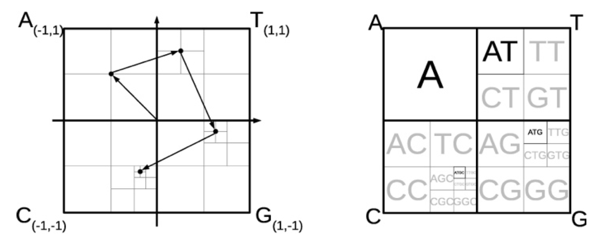
Table 1.
Simulated dataset, note: Individual is the number of sequences for each species; Seq. Length is the sequence length, and species is the number of species/classes.
Table 1.
Simulated dataset, note: Individual is the number of sequences for each species; Seq. Length is the sequence length, and species is the number of species/classes.
| Dataset | Ne | Individual | Seq. Length | Species |
| Ne1000 | 1000 | 20 | 650 | 50 |
| Ne10000 | 10000 | 20 | 650 | 50 |
| Ne50000 | 50000 | 20 | 650 | 50 |
Table 2.
The Six Real Datasets (Note: Training/Test Nums is the number of sequences divided into training and test sets; Seq. Length is the length of the sequences; Species is the number of species/classes; Gene Region are the DNA barcodes obtained from the gene regions).
Table 2.
The Six Real Datasets (Note: Training/Test Nums is the number of sequences divided into training and test sets; Seq. Length is the length of the sequences; Species is the number of species/classes; Gene Region are the DNA barcodes obtained from the gene regions).
| Dataset | Type | Training/Test Nums | Seq. Length | Species | Gene Region | Reference |
| Cypraeidae | Invertebrates | 1656 / 352 | 614 | 211 | COI | [14] |
| Drosophila | Invertebrates | 499 / 116 | 663 | 19 | COI | [15] |
| Inga | Plants | 786 / 122 | 1838 | 63 | trnD-trnT, ITS | [16] |
| Bats | Vertebrates | 695 / 144 | 659 | 96 | COI | [17] |
| Fishes | Vertebrates | 515 / 111 | 718 | 82 | COI | [18] |
| Birds | Vertebrates | 1306 / 317 | 691 | 150 | COI | [4] |
Table 3.
EUC obtained by CNN1.
| EUC-CNN1 | 1-Hot | 2-Mer | 2-Mer-p | 2-Me-p-All |
| Cypraeidae | 0.101 | 0.103 | 0.089 | 0.088 |
| Drosophila | 0.125 | 0.158 | 0.138 | 0.221 |
| Inga | 0.255 | 0.276 | 0.276 | 0.268 |
| Bats | 0 | 0 | 0 | 0 |
| Fishes | 0.123 | 0.118 | 0.135 | 0.135 |
| Birds | 0.050 | 0.043 | 0.059 | 0.057 |
| Average | 0.109 | 0.116 | 0.116 | 0.128 |
Table 4.
EUC obtained by CNN2.
| EUC-CNN2 | 1-Hot | 2-Mer | 2-Mer-p | 2-Me-p-All |
| Cypraeidae | 0.171 | 0.113 | 0.098 | 0.104 |
| Drosophila | 0.142 | 0.138 | 0.126 | 0.130 |
| Inga | 0.208 | 0.145 | 0.139 | 0.445 |
| Bats | 0 | 0 | 0 | 0 |
| Fishes | 0.127 | 0.122 | 0.127 | 0.110 |
| Birds | 0.052 | 0.097 | 0.059 | 0.084 |
| Average | 0.117 | 0.103 | 0.092 | 0.146 |
Table 5.
EUC obtained by different ensembles.
| CNN2 | CNN1 | CNN1+CNN2 | ATT | CNN1 + ATT | FCGR | CNN1 + ATT + FCGR | |
| Cypraeidae | 0.098 | 0.089 | 0.085 | 0.079 | 0.080 | 0.125 | 0.091 |
| Drosophila | 0.126 | 0.138 | 0.119 | 0.130 | 0.130 | 0.223 | 0.130 |
| Inga | 0.139 | 0.276 | 0.227 | 0.215 | 0.173 | 0.281 | 0.267 |
| Bats | 0 | 0 | 0 | 0 | 0 | 0 | 0 |
| Fishes | 0.127 | 0.135 | 0.117 | 0.123 | 0.135 | 0 | 0 |
| Birds | 0.059 | 0.059 | 0.053 | 0.030 | 0.045 | 0.119 | 0.045 |
| Average | 0.092 | 0.116 | 0.100 | 0.096 | 0.094 | 0.125 | 0.088 |
Table 6.
Accuracy obtained by different ensembles.
| Ac | CNN1 | CNN2 | CNN1+CNN2 | ATT | FCGR | CNN1+ATT | CNN1+ATT+FCGR |
| Cypraeidae | 96.88 | 96.31 | 96.59 | 96.31 | 96.31 | 96.59 | 96.59 |
| Drosophila | 99.14 | 99.14 | 99.14 | 99.14 | 99.14 | 99.14 | 99.14 |
| Inga | 93.39 | 92.56 | 93.39 | 93.39 | 95.04 | 94.21 | 95.04 |
| Bats | 100 | 100 | 100 | 100 | 100 | 100 | 100 |
| Fishes | 95.50 | 95.50 | 95.50 | 95.50 | 100 | 95.50 | 98.20 |
| Birds | 95.58 | 96.53 | 97.16 | 98.11 | 94.95 | 98.11 | 98.11 |
| Average | 96.74 | 96.67 | 96.96 | 97.07 | 97.57 | 97.25 | 97.85 |
Table 7.
Accuracy obtained using sequences aligned by MEGA.
| Ac | CNN1 | CNN2 | CNN1+CNN2 | ATT | FCGR | CNN1+ATT | CNN1+ATT+FCGR |
| Cypraeidae | 96.59 | 96.02 | 96.59 | 96.31 | 96.59 | 96.59 | 96.59 |
| Drosophila | 99.14 | 99.14 | 99.14 | 99.14 | 99.14 | 99.14 | 99.14 |
| Inga | 95.04 | 91.74 | 92.56 | 93.39 | 95.04 | 94.21 | 94.21 |
| Bats | 100 | 100 | 100 | 100 | 100 | 100 | 100 |
| Fishes | 100 | 100 | 100 | 100 | 100 | 100 | 100 |
| Birds | 97.16 | 96.53 | 97.48 | 97.48 | 94.95 | 98.11 | 98.11 |
| Average | 97.98 | 97.23 | 97.62 | 97.72 | 97.62 | 98.00 | 98.00 |
Table 8.
Mean and standard deviation of the EUC obtained by the 20 nets that belong to the ensemble of CNN1 or CNN2.
Table 8.
Mean and standard deviation of the EUC obtained by the 20 nets that belong to the ensemble of CNN1 or CNN2.
| EUC | CNN1 | CNN2 | ||
| mean | std | mean | std | |
| Cypraeidae | 0.168 | 0.048 | 0.158 | 0.957 |
| Drosophila | 0.162 | 0.043 | 0.116 | 0.013 |
| Inga | 0.599 | 0.252 | 0.620 | 0.214 |
| Bats | 0 | 0 | 0 | 0 |
| Fishes | 0.349 | 0.446 | 0.130 | 0.047 |
| Birds | 0.796 | 0.288 | 0.343 | 0.188 |
| Average | 0.346 | 0.179 | 0.228 | 0.236 |
Table 9.
Mean and standard deviation of the accuracy obtained by the 20 nets that belong to the ensemble of CNN1 or CNN2.
Table 9.
Mean and standard deviation of the accuracy obtained by the 20 nets that belong to the ensemble of CNN1 or CNN2.
| Ac | CNN1 | CNN2 | ||
| mean | std | mean | std | |
| Cypraeidae | 95.71 | 0.61 | 95.67 | 0.61 |
| Drosophila | 99.05 | 0.24 | 99.14 | 0 |
| Inga | 91.98 | 2.24 | 92.27 | 1.12 |
| Bats | 99.97 | 0.16 | 99.97 | 0.16 |
| Fishes | 95.36 | 0.33 | 95.23 | 0.54 |
| Birds | 90.68 | 1.51 | 93.64 | 1.44 |
| Average | 95.45 | 0.84 | 95.98 | 0.64 |
Table 10.
EUC obtained by SVM.
| SVM | 1-Hot | 2-Mer | 2-Mer-p |
| Cypraeidae | 0.104 | 0.124 | 0.115 |
| Drosophila | 0.470 | 0.454 | 0.430 |
| Inga | 1.767 | 1.361 | 1.443 |
| Bats | 0 | 0 | 0 |
| Fishes | 0.135 | 0.144 | 0.135 |
| Birds | 0.018 | 0.179 | 0.021 |
| Average | 0.416 | 0.377 | 0.357 |
Table 14.
F1 score performance.
| F1 score - Aligned data | CNN1 | ATT | CNN1 + ATT | FCGR | CNN1 + ATT + FCGR |
| Cypraeidae | 98.00 | 97.82 | 98.00 | 97.93 | 98.00 |
| Drosophila | 99.75 | 99.75 | 99.75 | 99.75 | 99.75 |
| Inga | 95.35 | 95.36 | 94.69 | 95.80 | 95.35 |
| Bats | 100 | 100 | 100 | 100 | 100 |
| Fishes | 100 | 100 | 100 | 100 | 100 |
| Birds | 97.94 | 98.67 | 98.99 | 97.49 | 98.99 |
| Average | 98.50 | 98.60 | 98.57 | 98.49 | 98.68 |
| F1 score - unaligned data |
CNN1 | ATT | CNN1 + ATT | FCGR | CNN1 + ATT + FCGR |
| Cypraeidae | 98.36 | 97.82 | 98.00 | 98.12 | 98.00 |
| Drosophila | 99.75 | 99.75 | 99.75 | 99.75 | 99.75 |
| Inga | 94.04 | 94.21 | 94.69 | 96.08 | 95.80 |
| Bats | 100 | 100 | 100 | 100 | 100 |
| Fishes | 96.08 | 96.54 | 96.08 | 100 | 99.35 |
| Birds | 96.94 | 99.11 | 99.11 | 97.34 | 99.11 |
| Average | 97.52 | 97.90 | 97.93 | 98.55 | 98.67 |
Disclaimer/Publisher’s Note: The statements, opinions and data contained in all publications are solely those of the individual author(s) and contributor(s) and not of MDPI and/or the editor(s). MDPI and/or the editor(s) disclaim responsibility for any injury to people or property resulting from any ideas, methods, instructions or products referred to in the content. |
© 2024 by the authors. Licensee MDPI, Basel, Switzerland. This article is an open access article distributed under the terms and conditions of the Creative Commons Attribution (CC BY) license (http://creativecommons.org/licenses/by/4.0/).
Copyright: This open access article is published under a Creative Commons CC BY 4.0 license, which permit the free download, distribution, and reuse, provided that the author and preprint are cited in any reuse.


