
Submitted:
20 September 2024
Posted:
20 September 2024
You are already at the latest version
Abstract
This paper compares Demand Response algorithms suitable for Short-term Forecasting based on Advanced Metering Infrastructure (AMI). It selects ARIMA (AutoRegressive Integrated Moving Average), SARIMA (Seasonal ARIMA), LSTM (Long Short-Term Memory), and SVM (Support Vector Machine) as the primary research algorithms and delves into their theoretical foundations and functional characteristics. The theoretical background section explores each algorithm’s applicability in analyzing time-series data, recognizing nonlinear patterns, and solving optimization and classification problems. The methodology section will detail the methods of AMI data collection, the implementation of the algorithms, and the experimental setup. In the experiments and results section, the performance of each algorithm will be assessed by applying AMI data and presenting the outcomes of comparative analyses, with a focus on evaluating the predictive accuracy of the algorithms. The discussion will interpret the experimental results, analyzing the advantages and disadvantages of each algorithm and their applicability in the AMI system. It will also explore the limitations of the current research and directions for future research. The conclusion will summarize the key findings of the study and affirm how this research contributes to understanding and improving short-term forecasting and demand response systems based on AMI.
Keywords:
Smart Grid
; Internet of Things
; SCADA
; AMI
; Demand Response
; ARIMA
; SARIMA
; LSTM
; SVM
; Short-term Forecasting
1. Introduction
Demand Response (DR) is one of the key components of the smart grid, designed to maintain the balance between electricity demand and supply and to improve the efficiency of the power grid [1]. Among the various structures of DR, the two most prominent are "Price-based Demand Response" and "Incentive-based Demand Response."
Price-based DR utilizes electricity price fluctuations to change consumers’ power consumption behaviors. It increases prices when the demand is high and decreases them when the demand is low, encouraging consumers to save electricity or adjust their consumption times. This approach includes Real-time Pricing (RTP) and Time-of-Use (TOU) pricing schemes [2].
Incentive-based DR manages the peak load of the power grid by providing economic incentives to consumers for reducing their power consumption or adjusting it to specific times. Notable examples include Demand Response Resources (DRR) and Capacity Market Payments [3,4].
Advanced Metering Infrastructure (AMI) is a fundamental component of the smart grid that significantly enhances the efficiency of Demand Response (DR) programs through real-time collection and analysis of electricity usage data [5]. AMI systems enable two-way communication between electricity consumers and utility companies, which is essential for the implementation of DR programs. Distributed DR systems play a crucial role in enhancing the resilience and reliability of the power grid, enabling rapid response times and optimizing energy management for individual users.
This study explores the applicability of various time series forecasting algorithms to enhance the efficiency of Demand Response based on Advanced Metering Infrastructure (AMI). It evaluates the capability of diverse algorithms such as ARIMA, SARIMA, LSTM, and SVM to handle the nonlinear patterns and volatility in electricity usage data. The comparative analysis of these algorithms aims to demonstrate that each has specific strengths in utilizing real-time AMI data to predict peak demand and manage loads effectively.
A key focus of this research is to strictly assess the prediction accuracy of models using real-time data, illustrating how certain algorithms can serve as powerful tools for utility companies to manage peak loads and dynamically optimize energy distribution in short-term forecasting scenarios. This analysis is expected to provide significant insights particularly for price-based Demand Response strategies like Real-time Pricing (RTP) and Time-of-Use (TOU). Additionally, it will provide evidence on how effectively incentive-based Demand Response strategies, which incentivize consumers through economic rewards to reduce power consumption, can be implemented.
The results of this study provide a foundation for future research directions and suggest the exploration of advanced machine learning techniques that can be integrated into smart grid infrastructures. Additionally, the findings offer practical implications for how algorithmic interventions can enhance the efficiency and reliability of Demand Response in establishing energy management policies.
To achieve this, this paper focuses on the selection of distributed DR methods using AMI and conducts a comparative analysis of short-term forecasting algorithms to choose the optimal demand response prediction algorithm.
2. Related work
Advanced Metering Infrastructure (AMI) represents a pivotal component of the smart grid. Its primary function encompasses tracking electricity consumption at client nodes and transmitting this information to utility centers. AMI undertakes roles in information collection, file storage, file transmission, bandwidth allocation, and billing issuance[6]. Additionally, Wang et al.[7] highlight the accuracy and reliability as significant advantages of demand response implementations in AMI systems.
- Accuracy: AMI-based demand response systems offer high precision in load control, contributing to efficient energy management and grid stability.
- Reliability: The centralized architecture and control strategies of AMI facilitate stable and trustworthy demand response operations, ensuring consistent performance.
However, smart meters within AMI are resource-constrained devices, characterized by limited computational and storage capabilities[8]. Moreover, a major challenge for AMI systems is their sustainability under unexpected usage patterns, low bandwidth, and significant informational performance degradation, with low-power-centric data technologies at the root of these issues[6]. Therefore, research in AMI functionalities must consider the constraints imposed by low-power-centric data technologies, particularly the limitations in computing and storage capabilities, which warrant serious consideration. Thus, determining the appropriate duration for data collection and analysis applied to demand response forecasting becomes crucial. While there is no standardized period for data collection and analysis for forecasting, various studies suggest differing durations: for Short Term Load Forecasting (STLF), the period ranges from less than a day to a week[9,10,11]; Medium Term Load Forecasting (MTLF) spans two weeks to three years[9,10,11]; and Long Term Load Forecasting (LTLF) encompasses three years to fifty years[9,11]. According to research by Hong et al. and Yunsun Kim et al., while no standard period exists, it is common to set STLF to less than a week, MTLF to one week to a month, and LTLF to more than a year[12,13]. Consequently, research into demand response in AMI must prioritize the selection of algorithms suitable for Short-term forecasting, considering the limitations of low-power-based technologies and the potential applicability of each algorithm to Short-term forecasting and demand response.
Recent research papers reveal that ARIMA and SARIMA models are effectively utilized in short-term forecasting, particularly in fields such as electric load forecasting and mobile network traffic predictions. These studies underscore the models’ efficacy in accurately predicting short-term variations across various sectors. For instance, research conducted by Kochetkova et al. employed SARIMA and other models for short-term forecasting of enterprise network traffic, demonstrating potential applicability in the electricity sector[14]. Minnaar et al. focused their research on using the SARIMA model for forecasting in electricity distribution, procurement, and sales, emphasizing the importance of accurate load forecasting for utility companies, especially in the context of increasing roles of renewable energy sources[15]. Moreover, studies like the one by Kien et al., which addressed SARIMA model usage for electric demand forecasting in Hanoi, showcase its effectiveness in predicting electricity demand in specific regions[16]. These examples demonstrate that ARIMA and SARIMA models are widely recognized and used across various sectors, making them highly relevant to research themes focusing on AMI and demand response.
Long Short-Term Memory (LSTM) models are deep learning models capable of effectively handling long-term dependencies in complex time series data. Developed to overcome the long-term dependency issues inherent in traditional Recurrent Neural Networks (RNNs), LSTMs have provided effective forecasting results in diverse areas, including electric load forecasting, stock market analysis, and weather condition predictions. A study by Al-Musaylh et al. (2018) that applied LSTM for electric demand forecasting illustrates the model’s capability in handling complex time series data[17]. Recent studies have explored LSTM’s approach to short-term forecasting across various fields. For example, research by Vatsa et al. employed LSTM for short-term forecasting of polarization current for transformer insulation assessment, extending LSTM architecture to capture long-term dependencies and complex temporal patterns[18].
Support Vector Machine (SVM) is another algorithm useful for short-term forecasting. Primarily known for classification problems, SVM is a robust machine learning technique that can also be applied to regression problems. It operates by mapping data features to a higher-dimensional space to find the optimal decision boundary. This characteristic makes it particularly valuable for short-term forecasting of nonlinear and complex data patterns. For instance, a study by Nepal et al. (2020) employing SVM for electric load forecasting demonstrated the model’s effectiveness in handling complex data patterns and providing accurate predictions[19].
However, existing studies tend to focus on implementing and examining a single algorithm. Hence, this paper aims to compare traditional time series analysis methods, such as ARIMA and SARIMA, with algorithms like LSTM and SVM, to enhance the efficiency of short-term forecasting in AMI systems. This comparison of diverse algorithms will play a crucial role in improving data processing and forecasting accuracy in AMI systems, ultimately contributing to better decision-making in energy management and planning.
3. Theoretical Background
3.1. ARIMA (AutoRegressive Integrated Moving Average)
The ARIMA model is a potent tool utilized for normalizing non-stationary trends in time series data and predicting future values. It combines AutoRegressive (AR) components, differencing (I) processes, and Moving Average (MA) components to analyze patterns and structures within time series data. ARIMA is applied across various fields, including economics, finance, and environmental science, showcasing exceptional performance in short-term forecasting in particular. The model identifies trends and seasonality in data over time, enabling accurate predictions[20,21].
The ARIMA model, used for analyzing time series data, is mathematically represented as follows:
3.2. SARIMA (Seasonal ARIMA)
SARIMA, an extension of the ARIMA model incorporating seasonal components, proves effective for data exhibiting seasonal patterns. This model integrates additional seasonal differencing and seasonal autoregressive elements into the conventional ARIMA model’s components. SARIMA is particularly beneficial for forecasting electric demand, analyzing stock markets, and researching climate change, adeptly modeling complex patterns in data with pronounced seasonal variability[22,23].
SARIMA model, an expansion of ARIMA to account for seasonal variability, is mathematically expressed as follows:
3.3. LSTM (Long Short-Term Memory)
LSTM, a variant of Recurrent Neural Networks (RNNs), was developed to address the issue of long-term dependencies in time series data. It can effectively learn patterns over time while maintaining important information over long periods in complex time series data. This capability has demonstrated LSTM’s potential in various fields, such as electric demand forecasting, stock market analysis, showcasing its application in areas requiring high accuracy in short-term and mid-term predictions[23,24].
The core components of LSTM and their mathematical structure are as follows:
-
Forget Gate
- (a)
- Decides the extent to which information from the previous state is retained.
-
Input Gate
- (a)
- Determines how much new information is added to the cell state.
-
Cell State Update
- (a)
- Updates the previous cell state to create a new cell state.
-
Output Gate
- (a)
- Determines which parts of the cell state are used to decide the next hidden state for output.
3.4. SVM (Support Vector Machine)
SVM is a robust machine learning algorithm widely used for solving classification and regression problems. It operates by mapping data to a higher-dimensional space and finding the optimal decision boundary. SVM is particularly effective for datasets with complex nonlinear relationships and is used in various fields, including electric demand forecasting, image classification, and bioinformatics. SVM maintains high performance even in high-dimensional data, accurately classifying and predicting complex patterns[25].
SVM classifies data by solving the following optimization problem:
4. Research Methodology
4.1. Application of Algorithms
This section meticulously delineates the implementation methodology for each of the selected time series forecasting algorithms.
4.1.1. ARIMA (AutoRegressive Integrated Moving Average)
The ARIMA model is employed to transform non-stationary time series data into a stationary form for future value predictions. The implementation of the ARIMA model encompasses the following steps:
-
Identify and preprocess time series data to remove trends and seasonality.
- (a)
- Removing Trends: Linear or nonlinear trends are eliminated from the data through differencing. The first differencing is calculated as:where is the observation at time t, and is the differenced time series.
- (b)
- Removing Seasonality: Seasonal differencing is applied to eliminate seasonal variations in the data, calculated over a period S:where S represents the seasonal period.
- (c)
- Checking Stationarity: After differencing, stationarity of the time series is tested using the ADF test. If the p-value is below 0.05, the series can be considered stationary.
- (d)
- Applying Transformations: Log transformation or Box-Cox transformation is applied to stabilize the variance of the data.
- (e)
- Analyzing ACF and PACF Plots: The parameters p, d, and q of the ARIMA model are determined by analyzing the ACF and PACF plots.
-
Analyze ACF and PACF plots to determine appropriate AR(p) and MA(q) parameters.
- (a)
- Analyzing ACF Plot: The ACF plot visualizes the correlation between observations in the time series data, showing the total correlation between lagged observations, and is used to estimate the order of the MA model (q). The cut-off point in the ACF plot after which correlations rapidly decrease can be chosen as the value for MA(q).
- (b)
- Analyzing PACF Plot: The PACF plot shows the correlation of individual lag values excluding the influence of other lag values, primarily used to determine the order of the AR model (p). The cut-off point in the PACF plot after which correlations rapidly decrease can be chosen as the value for AR(p).
- (c)
- Parameter Estimation: Based on ACF and PACF plots, the values of AR(p) and MA(q) best fitting the data are determined experimentally. Various combinations of p and q are tried, using information criteria (e.g., AIC, BIC) to select the optimal model.
-
Apply differencing (d) to make the data stationary and fit the ARIMA model to the data.
- (a)
- Differencing: Differencing in the ARIMA model is used to transform non-stationary time series data into a stationary form.
- (b)
- Model Fitting: Fit the ARIMA model to the differenced data. The ARIMA(p, d, q) model is defined as:
- (c)
- Model Estimation: Use optimization techniques to estimate the values of the model parameters and , evaluating the model’s fit and adjusting parameters as necessary.
- Validate the model’s stationarity using statistical tests like the ADF test.
-
Use the final model to predict future values and evaluate the model’s performance.
- (a)
- Predicting Future Values: Use the fitted ARIMA model to predict future values. The prediction is conducted using the model’s mathematical expression.
- (b)
- Evaluating Model Performance: Analyze the difference between predicted and actual values to evaluate the model’s performance. Common metrics include RMSE or MAE for performance evaluation.
- (c)
- Model Validation: Validate the model’s fit based on prediction performance, and adjust the model as necessary. Information criteria such as AIC or BIC can be used for comparison with other models.
Through these steps, the predictive capability of the ARIMA model is assessed, and its applicability to real-time series data is confirmed.
According to reference[23] elucidates the application of the ARIMA model to order demand forecasting, demonstrating the model’s applicability.
4.1.2. SARIMA (Seasonal ARIMA)
The SARIMA model extends the ARIMA model by incorporating seasonality, making it suitable for forecasting data with seasonal variations. The implementation of the SARIMA model includes the following steps:
-
Identify and preprocess time series data including seasonal elements.
- (a)
- Identify seasonal elements and preprocess the data accordingly. This involves capturing clear seasonal patterns in the time series data and normalizing them through differencing.
- (b)
- Apply seasonal differencing to normalize the data, defined as:where S is the seasonal period.
-
Determine the seasonal parameters (P, D, Q) of the SARIMA model based on the seasonal cycle (S).
- Decide on the seasonal parameters of the SARIMA model based on the seasonal cycle S, used to model periodic fluctuations in seasonal patterns.
- Analyze seasonal ACF and PACF plots to determine seasonal AR and MA parameters.
- Fit the model to the data and further adjust non-seasonal parameters (p, d, q) using ACF and PACF plots.
-
Evaluate the model’s fit through residual analysis and adjust the model if necessary.
- (a)
- Calculate residuals:where are the residuals, the observations, and the predictions.
- (b)
-
Assess statistical properties of residuals:
- Verify that the mean of the residuals is close to zero.
- Check for constant variance in the residuals (homoscedasticity).
- Examine residuals for autocorrelation using ACF and PACF.
- (c)
-
Normality test:
- Test whether the distribution of residuals follows a normal distribution (e.g., Shapiro-Wilk test).
Residual analysis evaluates the model’s fit and allows for adjustments to improve prediction accuracy. -
Generate forecasts considering seasonality using the final model. Predictions with the SARIMA model are made based on current and past data points and model parameters, estimating values for future points. The prediction formula is as follows:Where,
- is the forecast value at time .
- is the mean of the model.
- , , , are the seasonal and non-seasonal AR and MA parameters, respectively.
- and are past observations, and and are past error terms.
Using this formula, the SARIMA model predicts future values considering past data and seasonal patterns.
According to reference[24], the SARIMA model was highly effective in capturing seasonal patterns in time series data.
4.1.3. LSTM (Long Short-Term Memory)
LSTM is a deep learning-based time series prediction model capable of learning long-term dependencies in data. The implementation of the LSTM model includes the following steps:
-
Normalize the time series data and prepare it by dividing sequences into windows for feeding into the network.
- (a)
- Data Normalization: The process of normalizing data to enhance the efficiency of model training. Min-Max normalization is the most common method.where x is the original data value, and are the minimum and maximum values of the dataset, respectively.
- (b)
- Sequence Window Splitting: Time series data is divided into continuous sequences to be learnable by the network. Each sequence consists of a specific length of windows.where is the input sequence, is the value to be predicted at the next time point, and n is the window size.
-
Define the LSTM architecture, determining the number of layers and the number of neurons in each layer.
- (a)
- Number of Layers: The number of layers in the LSTM network determines the model’s depth, typically adjusted based on the complexity of the problem. Using more layers allows the model to learn more complex patterns but may increase the risk of overfitting.
- (b)
- Number of Neurons per Layer: The number of neurons in each LSTM layer determines the capacity of that layer. More neurons allow for storing more information but increase computational costs.
- (c)
-
Architecture Example:model = Sequential()model.add(LSTM(50,return_sequences=True,input_shape=(n_input, n_features)))model.add(LSTM(50,return_sequences=False))model.add(Dense(1))model.compile(optimizer=’adam’,loss=’mse’)In this example, two LSTM layers are used with 50 neurons each. `return_sequences=True` indicates that the output of the first layer is a sequence. The number of layers and neurons per layer should be optimized through experimentation to maintain a balance between performance and efficiency of the model.
-
Apply techniques to prevent overfitting using the prepared data.
- (a)
- (b)
-
Measures to prevent overfitting include the following methods:
- Validate the trained model’s performance, measuring prediction accuracy using evaluation metrics.
- Perform predictions on future data using the validated model.
Reference[24] presents a case of applying LSTM for time series forecasting, demonstrating LSTM’s ability to effectively learn and predict complex data patterns.
4.1.4. SVM (Support Vector Machine)
SVM is a powerful machine learning model used for time series forecasting, particularly effective in handling nonlinear and complex data patterns. It employs a risk function based on the principle of structural risk minimization to balance empirical error and regularization.
The implementation of SVM in short-term forecasting research based on AMI involves the following steps:
- Data Preparation: Preprocess and normalize AMI data to make it suitable for SVM.
- Model Development: Configure SVM using an appropriate kernel function to capture the complexity of the data.
- Training and Testing: Train the SVM model using historical AMI data and test its performance on unseen data.
- Performance Evaluation: Assess the model’s accuracy, speed, and efficiency using metrics appropriate for time series analysis.
Through this approach, SVM can be a useful tool in AMI systems for handling complex and nonlinear data patterns.
SVM is a powerful machine learning algorithm that defines a decision boundary based on the characteristics of the dataset, finding a hyperplane with the maximum margin to classify the given data. The basic form of SVM applies to linear classification problems, but it can be extended to nonlinear classification problems using the kernel trick.
The objective function of SVM is defined as follows:
Here, is the weight vector of the hyperplane, b is the bias, are slack variables, and C is the regularization parameter. This objective function aims to find a hyperplane that maximizes the margin and minimizes classification errors.
The kernel trick allows modeling complex nonlinear relationships by mapping the input space into a higher-dimensional feature space. The most commonly used kernel function is the Radial Basis Function (RBF):
Here, is the parameter of the RBF kernel, and and are feature vectors.
5. Experiments and Results
This section introduces the experimental methods and the data used for the experiments, along with presenting the results.
5.1. Experimental Methodology
The experiments in this research will be conducted as follows:
-
Collection and Trend Analysis of Time-Specific AMI Measurement Data: Collect data for training and analyze trends to understand the actual movements within the AMI measurement data.
- (a)
- Data collection for training
- (b)
- Data collection for comparison
- Applying Collected Data to Each Algorithm: The collected data is applied to each algorithm.
- Trend Comparison: The trends from the results of applying each algorithm are compared with previously observed trends to analyze differences.
- Data Comparison: Directly compare the data collected for comparison with the results from each algorithm to analyze the differences.
Through the above processes, the performance of each algorithm will be indirectly assessed to determine which algorithm performs best. Additionally, considering the operation based on AMI, the experiments will be conducted in a virtual environment configured with a 1Ghz 2core CPU and 800MB RAM.
5.2. Introduction to Experimental Data
KT, the National Information Society Agency (NIA), and the Ministry of Science and ICT of South Korea provide big data across various industrial sectors (https://www.bigdata-telecom.kr/). The big data used in this experiment are as follows:
-
Data for comparison: Time-specific AMI AI training data
- (a)
- Data period: December 1, 2021, to January 1, 2022
- (b)
- Data size: 5,426,322,257 Bytes
-
Data for training: Time-specific AMI electricity usage
- (a)
- Data period: July 1, 2021, to December 1, 2021
- (b)
- Data size: 15,479,044,282 Bytes
The data collected for final comparison is named "Time-specific AMI AI training data," and the data collected for training is named "Time-specific AMI electricity usage."
Table 1 defines the "Time-specific AMI AI training data" file, intending to verify the data and its trends based on the Consumer Number , Measurement Date , and Measurement Time .
5.3. Introduction to the Experimental Method for Learning AMI Time-Specific Power Usage Data
The collected "AMI Time-Specific Power Usage Data," like the previously collected "AMI Time-Specific AI Learning Data" for comparison, is provided in csv format, representing data measured in apartments equipped with actual AMI devices, organized by time of day. The data from July 1, 2021, to December 1, 2021, will be used for training each algorithm, and the results will be saved in csv files in the same format as the "AMI Time-Specific AI Learning Data" for direct comparison in the previous subsection "Collection and Trend Analysis of Time-Specific AMI Measurement Data." To facilitate this, data files from July 1, 2021, to December 1, 2021, were merged into one file, resulting in a csv file with a total size of 15,479,044,282 bytes and containing 316,712,453 lines. From this file, data for the 10 consumer numbers sampled in Figure 4 will be extracted. The definition of this recreated csv format can be found in Table 2.
The code to be implemented for the experiment and the hardware specifications on which the experiment will be conducted are as follows:
- Language: Python 3.11.7
-
Used Libraries
- (a)
- pandas
- (b)
- pmdarima
- (c)
- numpy
- (d)
- tqdm
- (e)
- datetime
- (f)
- sys
- (g)
- sklearn
- (h)
- tensorflow
-
Virtual Environment Hardware Specifications
- (a)
- CPU: 1.0GHz 2core
- (b)
- RAM: 800MB
5.4. ARIMA Algorithm Experiment and Results
Algorithm 1 presents the actual implementation, encompassing the majority of the steps involved in the implementation process of the proposed ARIMA model.
| Algorithm 1 Forecasting and Saving Power Usage Data Using ARIMA |
|
Table 3 summarizes the slope and intercept of the calculated trend lines for each consumer number .
5.5. SARIMA Algorithm Experiment and Results
Algorithm 2 presents the actual implementation, encompassing the majority of the steps involved in the implementation process of the proposed SARIMA model.
| Algorithm 2 Forecasting Power Usage with Seasonality and Saving the Results |
|
Table 4 summarizes the slope and intercept of the calculated trend lines for each consumer number .
5.6. LSTM Algorithm Experiment and Results
Algorithm 3 presents the actual implementation, encompassing the majority of the steps involved in the implementation process of the proposed LSTM model.
| Algorithm 3 Forecasting Power Usage with LSTM Model for Each Consumer Group |
|
Table 5 summarizes the slope and intercept of the calculated trend lines for each consumer number .
5.7. SVM (Support Vector Machine) Algorithm Experiment and Results
Algorithm 4 presents the actual implementation, encompassing the majority of the steps involved in the implementation process of the proposed SVM model.
| Algorithm 4 Predict Future Power Usage Using SVR Model |
|
Table 6 summarizes the slope and intercept of the calculated trend lines for each consumer number .
5.8. Experimental Results and Comparison
From Figure 5, Figure 6, Figure 7, Figure 8, Figure 9, Figure 10, Figure 11, Figure 12, Figure 13 and Figure 14, graphs feature a red zero line. This line indicates that the closer the predicted data, represented in blue, is to zero, the closer it is to the actual data. Furthermore, the predicted results for each consumer number will be quantitatively evaluated using three evaluation methods: MSE, MAE, and RMSE.
-
Mean Squared Error
- (a)
- The differences between actual and predicted values are squared, averaged, and then calculated.
- (b)
- (c)
- Here, represents the actual value, the predicted value, and n the number of samples. Since MSE squares the errors, it gives more weight to larger errors, making it a useful tool for emphasizing model performance in situations where larger errors are disadvantageous. Therefore, it has the characteristic of being more sensitive to larger errors [31].
-
Mean Absolute Error
- (a)
- Defined as the average of the absolute differences between the predicted values and the actual values.
- (b)
- (c)
- Unlike MSE, MAE evaluates model errors linearly, making it less sensitive to larger errors. Therefore, this characteristic makes it a metric that can be used when all errors need to be treated uniformly. It differentiates itself from MSE by treating all errors equally [31].
-
Root Mean Squared Error
- (a)
- By taking the square root of MSE, the utility of MSE can be further extended, thereby restoring the error metric to the same scale as the predicted data.
- (b)
- (c)
- RMSE combines the sensitivity of MSE to large errors with the advantage of being in the same units as the response variable, making it an essential metric for comparing and evaluating various regression models on a consistent scale [31].
In the domain of predictive modeling and data analysis, the Mean Squared Error (MSE), Mean Absolute Error (MAE), and Root Mean Squared Error (RMSE) serve as fundamental metrics for evaluating the performance and accuracy of regression models. Each metric offers a distinctive approach to quantifying and analyzing the discrepancies between the model’s predicted values and the actual observed data, thereby enabling a robust understanding of the model’s effectiveness in relation to empirical data. Algorithm 5 represents the implementation code for each analysis method.
| Algorithm 5 Calculate Error Metrics per CNSMR_NO |
|
Figures illustrating the differences between predicted and actual data, and Algorithm 5 employing each algorithm’s predicted and actual data to assess accuracy using the MSE, MAE, and RMSE methods, are followed by tables summarizing the evaluation metrics. The overall analysis based on these evaluation metrics yields the following results.
-
Consumer Number (CNSMR_NO): DJ0200309001501
- (a)
- Figure 5: Graphs illustrating the differences between algorithm-specific predicted and actual data
- (b)
- Table 7: Accuracy evaluation for the predicted data using MSE, MAE, RMSE
- (c)
-
Algorithm-specific evaluation results according to Table 7
- ARIMA: With results of MSE , MAE , RMSE , demonstrating performance comparable to SARIMA.
- SARIMA: Exhibiting MSE , MAE , RMSE , indicating performance second only to SVM.
- LSTM: Showing the highest error values with MSE , MAE , RMSE , indicating the lowest prediction accuracy for this dataset.
- SVM: Achieving the lowest MSE , MAE , RMSE , signifying the most accurate predictions for this dataset.
-
Consumer Number (CNSMR_NO): DJ0800133001204
- (a)
- Figure 6: Graphs illustrating the differences between algorithm-specific predicted and actual data
- (b)
- Table 8: Accuracy evaluation for the predicted data using MSE, MAE, RMSEfor each algorithm
- (c)
-
Evaluation results for each algorithm based on Table 8
- ARIMA: With MSE , MAE , and RMSE , showing similar performance to SARIMA.
- SARIMA: Shows slightly higher error rates than ARIMA with MSE , MAE , and RMSE , positioning it as second-best after SVM.
- LSTM: Recorded the highest error rates with MSE , MAE , and RMSE , indicating the lowest prediction accuracy for this dataset.
- SVM: Exhibited the lowest error rates with MSE , MAE , and RMSE , signifying the most accurate predictions for this dataset.
-
Consumer Number (CNSMR_NO): DJ1200215000404
- (a)
- Figure 7: Graphs illustrating the differences between algorithm-specific predicted and actual data
- (b)
- Table 9: Accuracy evaluation for the predicted data using MSE, MAE, RMSEfor each algorithm
- (c)
-
Evaluation results for each algorithm based on Table 9
- ARIMA: Demonstrates similar performance to SARIMA with MSE , MAE , and RMSE , indicating closely matching results down to several decimal places.
- SARIMA: Exhibits comparable results to ARIMA, positioning it as effective after SVM in terms of performance.
- LSTM: Shows the highest error rates with MSE , MAE , and RMSE , indicating the lowest prediction accuracy for this dataset.
- SVM: Achieves the lowest error rates with MSE , MAE , and RMSE , signifying the most accurate predictions for this dataset.
-
Consumer Number (CNSMR_NO): CB0100106000505
- (a)
- Figure 8: Graphs illustrating the differences between algorithm-specific predicted and actual data
- (b)
- Table 10: Accuracy evaluation for the predicted data using MSE, MAE, RMSEfor each algorithm
- (c)
-
Evaluation results for each algorithm based on Table 10
- ARIMA: Recorded the highest error with MSE , MAE , and RMSE .
- SARIMA: Demonstrates slightly better performance than ARIMA with MSE , MAE , and RMSE , making it second-best after SVM.
- LSTM: Shows marginally higher error than SARIMA with MSE , MAE , and RMSE for this dataset.
- SVM: Exhibited the lowest error rates with MSE , MAE , and RMSE , indicating the most accurate predictions for this dataset.
-
Consumer Number (CNSMR_NO): CN0100107001801
- (a)
- Figure 9: Graphs illustrating the differences between algorithm-specific predicted and actual data
- (b)
- Table 11: Accuracy evaluation for the predicted data using MSE, MAE, RMSEfor each algorithm
- (c)
-
Evaluation results for each algorithm based on Table 11
- ARIMA: Exhibited MSE , MAE , and RMSE , showing very similar performance to SARIMA.
- SARIMA: Recorded MSE , MAE , and RMSE , providing the most accurate predictions for this dataset.
- LSTM: Demonstrated the highest error rates with MSE , MAE , and RMSE for this dataset.
- SVM: Showed slightly higher error rates with MSE , MAE , and RMSE compared to ARIMA and SARIMA, but remained close in prediction accuracy.
-
Consumer Number (CNSMR_NO): CN0200311001801
- (a)
- Figure 10: Graphs illustrating the differences between algorithm-specific predicted and actual data
- (b)
- Table 12: Accuracy evaluation for the predicted data using MSE, MAE, RMSEfor each algorithm
- (c)
-
Evaluation results for each algorithm based on Table 12
- ARIMA: Displayed MSE , MAE , and RMSE , showing nearly identical performance to SARIMA.
- SARIMA: Also recorded MSE , MAE , and RMSE , demonstrating performance second only to SVM.
- LSTM: Had the highest error rates with MSE , MAE , and RMSE for this dataset.
- SVM: Achieved the lowest error rates with MSE , MAE , and RMSE , indicating the most accurate predictions for this dataset.
-
Consumer Number (CNSMR_NO): CN1100106000103
- (a)
- Figure 11: Graphs illustrating the differences between algorithm-specific predicted and actual data
- (b)
- Table 13: Accuracy evaluation for the predicted data using MSE, MAE, RMSEfor each algorithm
- (c)
-
Evaluation results for each algorithm based on Table 13
- ARIMA: Demonstrated MSE , MAE , RMSE .
- SARIMA: Showed identical performance to ARIMA with MSE , MAE , RMSE .
- LSTM: Recorded the highest error rates with MSE , MAE , RMSE in this dataset.
- SVM: Achieved the lowest error rates with MSE , MAE , RMSE , providing the most accurate predictions for this dataset.
-
Consumer Number (CNSMR_NO): CN1600102001004
- (a)
- Figure 12: Graphs illustrating the differences between algorithm-specific predicted and actual data
- (b)
- Table 14: Accuracy evaluation for the predicted data using MSE, MAE, RMSEfor each algorithm
- (c)
-
Evaluation results for each algorithm based on Table 14
- ARIMA: Reported MSE , MAE , and RMSE .
- SARIMA: Exhibited identical performance to ARIMA with MSE , MAE , and RMSE .
- LSTM: Recorded the highest error rates with MSE , MAE , and RMSE for this dataset.
- SVM: Achieved the lowest error rates with MSE , MAE , and RMSE , providing the most accurate predictions for this dataset.
-
Consumer Number (CNSMR_NO): CN0500311000403
- (a)
- Figure 13: Graphs illustrating the differences between algorithm-specific predicted and actual data
- (b)
- Table 15: Accuracy evaluation for the predicted data using MSE, MAE, RMSEfor each algorithm
- (c)
-
Evaluation results for each algorithm based on Table 15
- ARIMA: Exhibited MSE , MAE , and RMSE , indicating the highest error values for this dataset.
- SARIMA: Reported MSE , MAE , and RMSE , showing slightly higher errors compared to SVM.
- LSTM: Achieved the lowest error rates with MSE , MAE , and RMSE , providing the most accurate predictions for this dataset.
- SVM: Recorded MSE , MAE , and RMSE , demonstrating the second-best performance after LSTM.
-
Consumer Number (CNSMR_NO): CN0700109000102
- (a)
- Figure 14: Graphs illustrating the differences between algorithm-specific predicted and actual data
- (b)
- Table 16: Accuracy evaluation for the predicted data using MSE, MAE, RMSEfor each algorithm
- (c)
-
Evaluation results for each algorithm based on Table 16
- ARIMA: Achieved MSE , MAE , RMSE , providing the most accurate predictions for this dataset.
- SARIMA: Recorded identical performance to ARIMA with MSE , MAE , RMSE .
- LSTM: Showed slightly higher error rates with MSE , MAE , RMSE compared to ARIMA and SARIMA.
- SVM: Reported the highest error rates with MSE , MAE , RMSE for this dataset.
Figure 15 illustrates the overall differences in SGPowerUsage values between the predictions and actual data for each model . For reference, each graph includes a red dotted zero line. Points above this line indicate an overestimation by the model, while points below indicate an underestimation.
- ARIMA: Exhibits performance similar to SARIMA but with a slightly higher MAE.
- SARIMA: Generally closer to the zero line compared to LSTM, though with some deviations, which are reflected in the MAE.
- LSTM: Shows larger deviations from the zero line, resulting in a higher MAE compared to other models.
- SVM: Demonstrates relatively small fluctuations around the zero line, indicating predictions closer to the actual values, consistent with the lowest MAE.
Based on the overall experimental results, it can be concluded that SVM is the most accurate algorithm for scenarios like short-term forecasting in AMI, where the dataset is small or limited resources are available for prediction.
6. Discussion
In this study, the performance of four predictive models, SVM, ARIMA, SARIMA, and LSTM, was evaluated across various time series datasets, aiming to improve the accuracy of predicting actual electricity usage . The results were derived using statistical metrics such as Mean Squared Error , Mean Absolute Error , and Root Mean Squared Error .
Initially, the expected performance ranking of the algorithms "ARIMA", "SARIMA", "LSTM", "SVM", and the rationale were as follows:
- LSTM: Given its capability to learn long-term dependencies in time series data and model complex patterns and nonlinearity, LSTM was anticipated to be highly effective, especially with large datasets containing more information and patterns. Additionally, LSTM can efficiently process large datasets using GPU acceleration, making it feasible for learning from substantial data given adequate computing resources [32,33].
- SVM: Useful for classifying or regressing nonlinear patterns in high-dimensional spaces through kernel tricks, SVM might be slower than LSTM for large datasets but can effectively model specific nonlinear patterns. Its flexibility with various kernel functions allows for adaptive transformation of data features, capturing the characteristics of time series data more accurately [34,35].
- SARIMA: Specialized in analyzing time series data with seasonality, SARIMA could effectively model this aspect in large datasets with clear seasonal patterns. It is interpretable and allows for a clear understanding of the seasonal patterns and trends in the data through its modeling results [36].
- ARIMA: Strong in modeling non-seasonal linear time series data, ARIMA could be useful for datasets primarily exhibiting linear patterns, although it might be less suitable for datasets with seasonality or nonlinear patterns. Despite potential limitations in processing large datasets, ARIMA’s relatively simple computations for model construction and prediction could be advantageous in scenarios with limited computing resources [37].
- Conclusion: Understanding the characteristics and requirements of the data accurately and selecting the appropriate model is crucial. While LSTM might be most promising for large datasets, SARIMA or SVM could be considered for clear modeling of seasonality or specific patterns. ARIMA could be more suitable for simpler time series data.
However, the outcomes of this research showed that the Support Vector Machine model exhibited the most superior prediction performance across most datasets by recording the lowest error metrics. This can be attributed to SVM’s excellent capability in handling complex nonlinear patterns and its superior generalization ability. In particular, SVM leveraged the kernel trick to effectively process data characteristics in high-dimensional spaces, demonstrating exceptional performance in capturing the complex structures and dynamics within time series data [38].
Meanwhile, Autoregressive Integrated Moving Average and Seasonal Autoregressive Integrated Moving-Average models exhibited strengths in modeling the seasonality and trends of time series data but showed relatively higher error metrics compared to SVM. This indicates that while ARIMA and SARIMA models can effectively reflect linear trends in time series data, they have limitations in modeling nonlinear patterns and complex interactions within the data [39].
The Long Short-Term Memory model demonstrated outstanding prediction performance in certain datasets but did not consistently exhibit good performance. The performance of LSTM significantly depends on having sufficient training data and proper hyperparameter settings [40,41,42], suggesting that these conditions might not have been optimized in this study.
Moreover, when comparing "ARIMA", "SARIMA", "LSTM", "SVM" algorithms directly in scenarios with limited resources and small datasets for training, such as AMI, it’s crucial to consider various aspects of performance and efficiency, including data processing capabilities, model complexity, training time, prediction performance, and memory management.
- ARIMA and SARIMA: As traditional time series analysis methods, they can be relatively fast and efficient in processing large datasets. However, their computational complexity may increase with the size of the time units in the data, and estimating the model’s parameters in large datasets can be time-consuming.
- LSTM: Possesses a strong capability to learn long-term dependencies and complex patterns in very large datasets. Training LSTM on very large datasets, however, can be computationally expensive and time-consuming.
- SVM: While effective at handling nonlinear patterns, learning times and memory requirements can significantly increase for large datasets.
7. Conclusion
This study aimed to evaluate the performance of various time series prediction models and conduct an in-depth analysis of each model’s strengths and weaknesses to contribute to selecting appropriate predictive models for real-world problems like electricity usage forecasting in AMI. Based on the research findings, choosing the right model based on the characteristics of the data and the prediction goals is crucial. Moreover, to improve the prediction accuracy for complex time series data, optimizing the model’s hyperparameters and considering the application of ensemble techniques combining various models in AMI should be explored.
Based on the results of this study, the combinations expected to enhance performance and accuracy in AMI when algorithms are combined are as follows:
- SARIMA + SVM combination or ARIMA + SVM combination: SARIMA or ARIMA can handle the linear or seasonal patterns in time series data, while SVM can complement nonlinear patterns. Especially as observed in this study, SVM can be useful for analyzing nonlinear patterns in small datasets or specific time segments. A strategy of training and predicting models targeting specific segments of the data can be employed.
- LSTM + SARIMA combination: LSTM has excellent capabilities in learning nonlinear patterns and long-term dependencies, while SARIMA can model clear patterns like seasonality. LSTM can be used to learn complex patterns, and SARIMA to complement seasonal patterns. However, this combination may require very high resource usage.
For short-term forecasting of demand response in AMI, both the model’s performance and efficiency must be considered. LSTM has strengths in learning complex nonlinear patterns but requires high resources for learning on large datasets. Conversely, ARIMA and SARIMA have relatively low computational costs but limited capabilities in learning nonlinear patterns. SVM can be useful for nonlinear patterns. Therefore, selecting or combining the appropriate model(s) based on the characteristics of the data and the requirements of the prediction task is crucial.
Future studies should further investigate the SARIMA + SVM combination or the ARIMA + SVM combination and the LSTM + SARIMA combination to analyze the accuracy achieved with these combinations and compare the resource usage related to accuracy improvements. This will help more accurately select the most suitable methodology for short-term forecasting of demand response in AMI. Additionally, while this research utilized datasets in a simulated environment rather than actual AMI, subsequent studies should aim to derive more in-depth and specific results using limited resources in actual AMI environments. This will contribute to selecting appropriate predictive models for real-world problems like electricity usage forecasting in AMI.
References
- Li, Y.; Han, M.; Yang, Z.; Li, G. Coordinating Flexible Demand Response and Renewable Uncertainties for Scheduling of Community Integrated Energy Systems With an Electric Vehicle Charging Station: A Bi-Level Approach. IEEE Transactions on Sustainable Energy 2021, 12, 2321–2331. [Google Scholar] [CrossRef]
- Wang, Z.; Paranjape, R.; Chen, Z.; Zeng, K. Layered stochastic approach for residential demand response based on real-time pricing and incentive mechanism. IET Generation, Transmission & Distribution 2020, 14, 423–431. [Google Scholar] [CrossRef]
- Asensio, M.; Meneses de Quevedo, P.; Muñoz-Delgado, G.; Contreras, J. Joint Distribution Network and Renewable Energy Expansion Planning Considering Demand Response and Energy Storage—Part I: Stochastic Programming Model. IEEE Transactions on Smart Grid 2018, 9, 655–666. [Google Scholar] [CrossRef]
- Sun, J.; Liu, J.; Chen, H.; He, P.; Yuan, H.; Yan, Z. Experiences and Lessons Learned From DR Resources Participating in the US and UK Capacity Markets: Mechanisms, Status, Dilemmas and Recommendations. IEEE Access 2022, 10, 83851–83868. [Google Scholar] [CrossRef]
- Zanghi, E.; Brown Do Coutto Filho, M.; Stacchini de Souza, J.C. Collaborative smart energy metering system inspired by blockchain technology. International Journal of Innovation Science 2023, 16, 227–243. [Google Scholar] [CrossRef]
- Anupong, W.; Azhagumurugan, R.; Sahay, K.B.; Dhabliya, D.; Kumar, R.; Vijendra Babu, D. Towards a high precision in AMI-based smart meters and new technologies in the smart grid. Sustainable Computing: Informatics and Systems 2022, 35, 100690. [Google Scholar] [CrossRef]
- Wang, Q.; Wang, H.; Zhu, L.; Wu, X.; Tang, Y. A Multi-Communication-Based Demand Response Implementation Structure and Control Strategy. Applied Sciences 2019, 9, 3218. [Google Scholar] [CrossRef]
- Le, T.N.; Chin, W.L.; Truong, D.K.; Hiep Nguyen, T.; Le, T.N.; Chin, W.L.; Truong, D.K.; Hiep Nguyen, T. Advanced Metering Infrastructure Based on Smart Meters in Smart Grid. In Smart Metering Technology and Services - Inspirations for Energy Utilities; IntechOpen, 2016. [CrossRef]
- Tao, H.; Shahidehpour, M. Load Forecasting: Case Study, 2015.
- Kyriakides, E.; Polycarpou, M. Short Term Electric Load Forecasting: A Tutorial. In Trends in Neural Computation; Chen, K., Wang, L., Eds.; Studies in Computational Intelligence, Springer: Berlin, Heidelberg, 2007; pp. 391–418. [Google Scholar] [CrossRef]
- Burg, L.; Gürses-Tran, G.; Madlener, R.; Monti, A. Comparative Analysis of Load Forecasting Models for Varying Time Horizons and Load Aggregation Levels. Energies 2021, 14, 7128. [Google Scholar] [CrossRef]
- Hong, T.; Fan, S. Probabilistic electric load forecasting: A tutorial review. International Journal of Forecasting 2016, 32, 914–938. [Google Scholar] [CrossRef]
- Kim, Y.; Son, H.g.; Kim, S. Short term electricity load forecasting for institutional buildings. Energy Reports 2019, 5, 1270–1280. [Google Scholar] [CrossRef]
- Kochetkova, I.; Kushchazli, A.; Burtseva, S.; Gorshenin, A. Short-Term Mobile Network Traffic Forecasting Using Seasonal ARIMA and Holt-Winters Models. Future Internet 2023, 15, 290. [Google Scholar] [CrossRef]
- MINNAAR, M.; HICKS, M.V.Z. Applied SARIMA Models for Forecasting Electricity Distribution Purchases and Sales.
- Kien, D.; Huong, P.; Minh, N. Application of Sarima Model in Load Forecasting in Hanoi City. International Journal of Energy Economics and Policy 2023, 13, 164–170. [Google Scholar] [CrossRef]
- Al Musaylh, M.S.; Deo, R.C.; Adamowski, J.F.; Li, Y. Short-term electricity demand forecasting with MARS, SVR and ARIMA models using aggregated demand data in Queensland, Australia. Advanced Engineering Informatics 2018, 35, 1–16. [Google Scholar] [CrossRef]
- Vatsa, A.; Hati, A.S.; Kumar, P.; Margala, M.; Chakrabarti, P. Residual LSTM-based short duration forecasting of polarization current for effective assessment of transformers insulation. Scientific Reports 2024, 14, 1369. [Google Scholar] [CrossRef]
- Nepal, B.; Yamaha, M.; Yokoe, A.; Yamaji, T. Electricity load forecasting using clustering and ARIMA model for energy management in buildings. JAPAN ARCHITECTURAL REVIEW 2020, 3, 62–76. [Google Scholar] [CrossRef]
- Hui, H.; Ding, Y.; Shi, Q.; Li, F.; Song, Y.; Yan, J. 5G network-based Internet of Things for demand response in smart grid: A survey on application potential. Applied Energy 2020, 257, 113972. [Google Scholar] [CrossRef]
- Tarmanini, C.; Sarma, N.; Gezegin, C.; Ozgonenel, O. Short term load forecasting based on ARIMA and ANN approaches. Energy Reports 2023, 9, 550–557. [Google Scholar] [CrossRef]
- Conejo, A.J.; Morales, J.M.; Baringo, L. Real-Time Demand Response Model. IEEE Transactions on Smart Grid 2010, 1, 236–242. [Google Scholar] [CrossRef]
- Wang, C.C.; Chien, C.H.; Trappey, A.J.C. On the Application of ARIMA and LSTM to Predict Order Demand Based on Short Lead Time and On-Time Delivery Requirements. Processes 2021, 9, 1157. [Google Scholar] [CrossRef]
- Kumar Dubey, A.; Kumar, A.; García-Díaz, V.; Kumar Sharma, A.; Kanhaiya, K. Study and analysis of SARIMA and LSTM in forecasting time series data. Sustainable Energy Technologies and Assessments 2021, 47, 101474. [Google Scholar] [CrossRef]
- Ruiz-Abellón, M.C.; Fernández-Jiménez, L.A.; Guillamón, A.; Falces, A.; García-Garre, A.; Gabaldón, A. Integration of Demand Response and Short-Term Forecasting for the Management of Prosumers’ Demand and Generation. Energies 2020, 13, 11. [Google Scholar] [CrossRef]
- Bouktif, S.; Fiaz, A.; Ouni, A.; Serhani, M.A. Optimal Deep Learning LSTM Model for Electric Load Forecasting using Feature Selection and Genetic Algorithm: Comparison with Machine Learning Approaches †. Energies 2018, 11, 1636. [Google Scholar] [CrossRef]
- Parvandeh, S.; Yeh, H.W.; Paulus, M.P.; McKinney, B.A. Consensus features nested cross-validation. Bioinformatics 2020, 36, 3093–3098. [Google Scholar] [CrossRef] [PubMed]
- Ookura, S.; Mori, H. An Efficient Method for Wind Power Generation Forecasting by LSTM in Consideration of Overfitting Prevention. IFAC-PapersOnLine 2020, 53, 12169–12174. [Google Scholar] [CrossRef]
- Shi, Q.; Zhang, H. Fault Diagnosis of an Autonomous Vehicle With an Improved SVM Algorithm Subject to Unbalanced Datasets. IEEE Transactions on Industrial Electronics 2021, 68, 6248–6256. [Google Scholar] [CrossRef]
- Sun, H.; Fan, M.; Sharma, A. Design and implementation of construction prediction and management platform based on building information modelling and three-dimensional simulation technology in Industry 4.0. IET Collaborative Intelligent Manufacturing 2021, 3, 224–232. [Google Scholar] [CrossRef]
- Stajkowski, S.; Kumar, D.; Samui, P.; Bonakdari, H.; Gharabaghi, B. Genetic-Algorithm-Optimized Sequential Model for Water Temperature Prediction. Sustainability 2020, 12, 5374. [Google Scholar] [CrossRef]
- Sirisha, U.M.; Belavagi, M.C.; Attigeri, G. Profit Prediction Using ARIMA, SARIMA and LSTM Models in Time Series Forecasting: A Comparison. IEEE Access 2022, 10, 124715–124727. [Google Scholar] [CrossRef]
- Nagendra, B.; Singh, G. Comparing ARIMA, Linear Regression, Random Forest, and LSTM for Time Series Forecasting: A Study on Item Stock Predictions. 2023 4th IEEE Global Conference for Advancement in Technology (GCAT), 2023, pp. 1–8. [CrossRef]
- Pathrikar, V.; Podutwar, T.; Vispute, S.R.; Siddannavar, A.; Mandana, A.; Rajeswari, K. Forecasting Diurnal Covid-19 Cases for Top-5 Countries Using Various Time-series Forecasting Algorithms. 2022 International Conference on Emerging Smart Computing and Informatics (ESCI), 2022, pp. 1–6. [CrossRef]
- Yang, S.F.; Choi, S.W.; Lee, E.B. A Prediction Model for Spot LNG Prices Based on Machine Learning Algorithms to Reduce Fluctuation Risks in Purchasing Prices. Energies 2023, 16, 4271. [Google Scholar] [CrossRef]
- Shiwakoti, R.K.; Charoenlarpnopparut, C.; Chapagain, K. Time Series Analysis of Electricity Demand Forecasting Using Seasonal ARIMA and an Exponential Smoothing Model. 2023 International Conference on Power and Renewable Energy Engineering (PREE), 2023, pp. 131–137.
- Imani, M. Sea level prediction using time series obtained from satellite altimetry observations. thesis, 2014. Accepted: 2023-03-16T06:44:06Z Journal Abbreviation: Sea level prediction using time series obtained from satellite altimetry observations.
- Leong, W.C.; Kelani, R.O.; Ahmad, Z. Prediction of air pollution index (API) using support vector machine (SVM). Journal of Environmental Chemical Engineering 2020, 8, 103208. [Google Scholar] [CrossRef]
- Wang, Y.; Xu, C.; Yao, S.; Wang, L.; Zhao, Y.; Ren, J.; Li, Y. Estimating the COVID-19 prevalence and mortality using a novel data-driven hybrid model based on ensemble empirical mode decomposition. Scientific Reports 2021, 11, 21413. [Google Scholar] [CrossRef] [PubMed]
- Liu, S.; Wan, Y.; Yang, W.; Tan, A.; Jian, J.; Lei, X. A Hybrid Model for Coronavirus Disease 2019 Forecasting Based on Ensemble Empirical Mode Decomposition and Deep Learning. International Journal of Environmental Research and Public Health 2023, 20, 617. [Google Scholar] [CrossRef] [PubMed]
- Hashemi, R.; Brigode, P.; Garambois, P.A.; Javelle, P. How can we benefit from regime information to make more effective use of long short-term memory (LSTM) runoff models? Hydrology and Earth System Sciences 2022, 26, 5793–5816. [Google Scholar] [CrossRef]
- Lan, X.; Li, Y.; Su, Y.; Meng, L.; Kong, X.; Xu, T. Performance degradation prediction model of rolling bearing based on self-checking long short-term memory network. Measurement Science and Technology 2022, 34, 015016. [Google Scholar] [CrossRef]
Figure 1.
Possibility of overfitting due to amount of learning data.
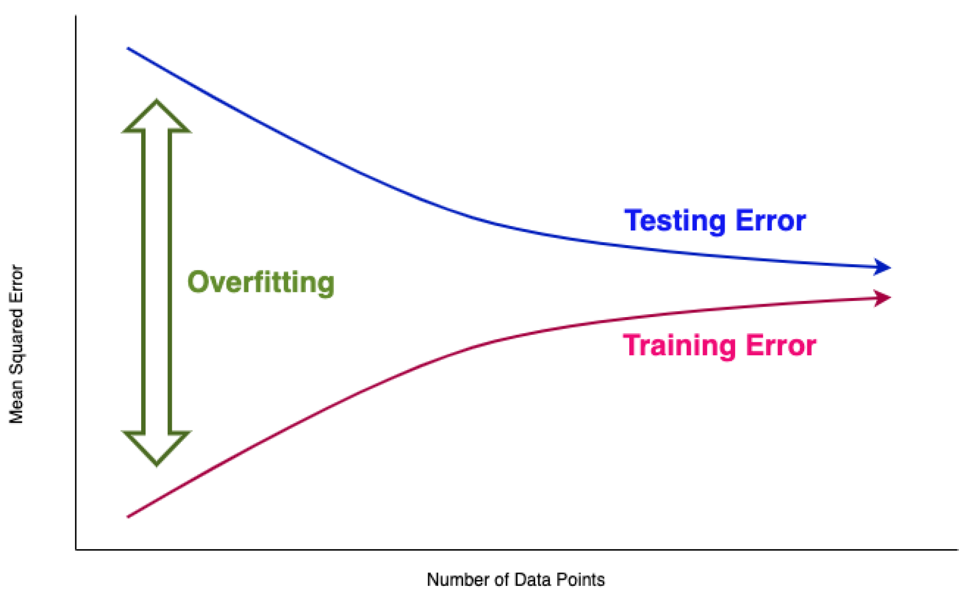
Figure 2.
Neural network without dropout.

Figure 3.
Neural network with dropout.
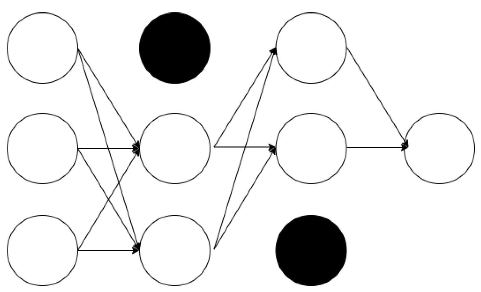
Figure 4.
Distribution and trend line graphs of sampled data by Consumer Number (CNSMR_NO).
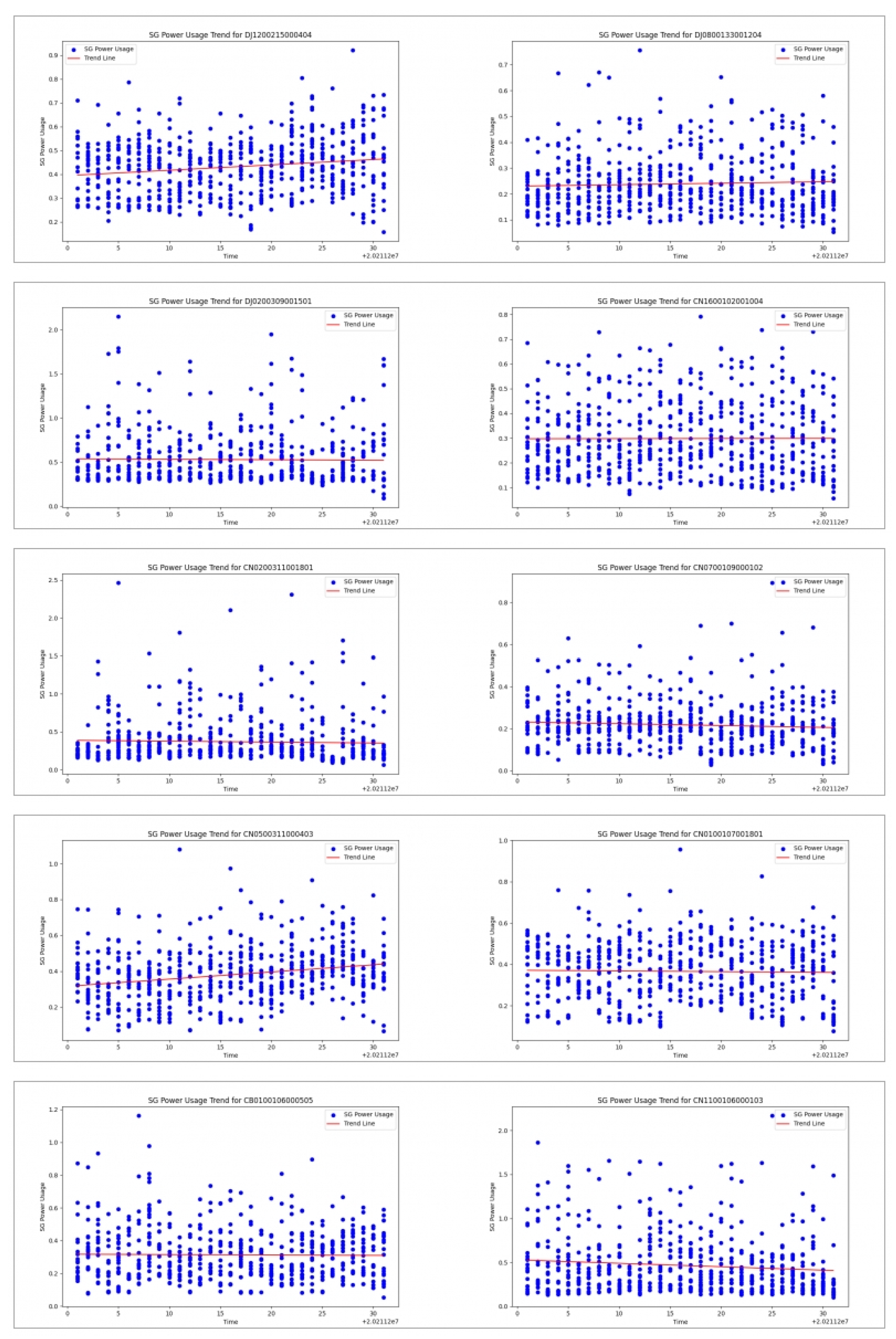
Figure 5.
Differences in SGPowerUsage Values Between Predictions and Actual Data in DJ0200309001501.
Figure 5.
Differences in SGPowerUsage Values Between Predictions and Actual Data in DJ0200309001501.
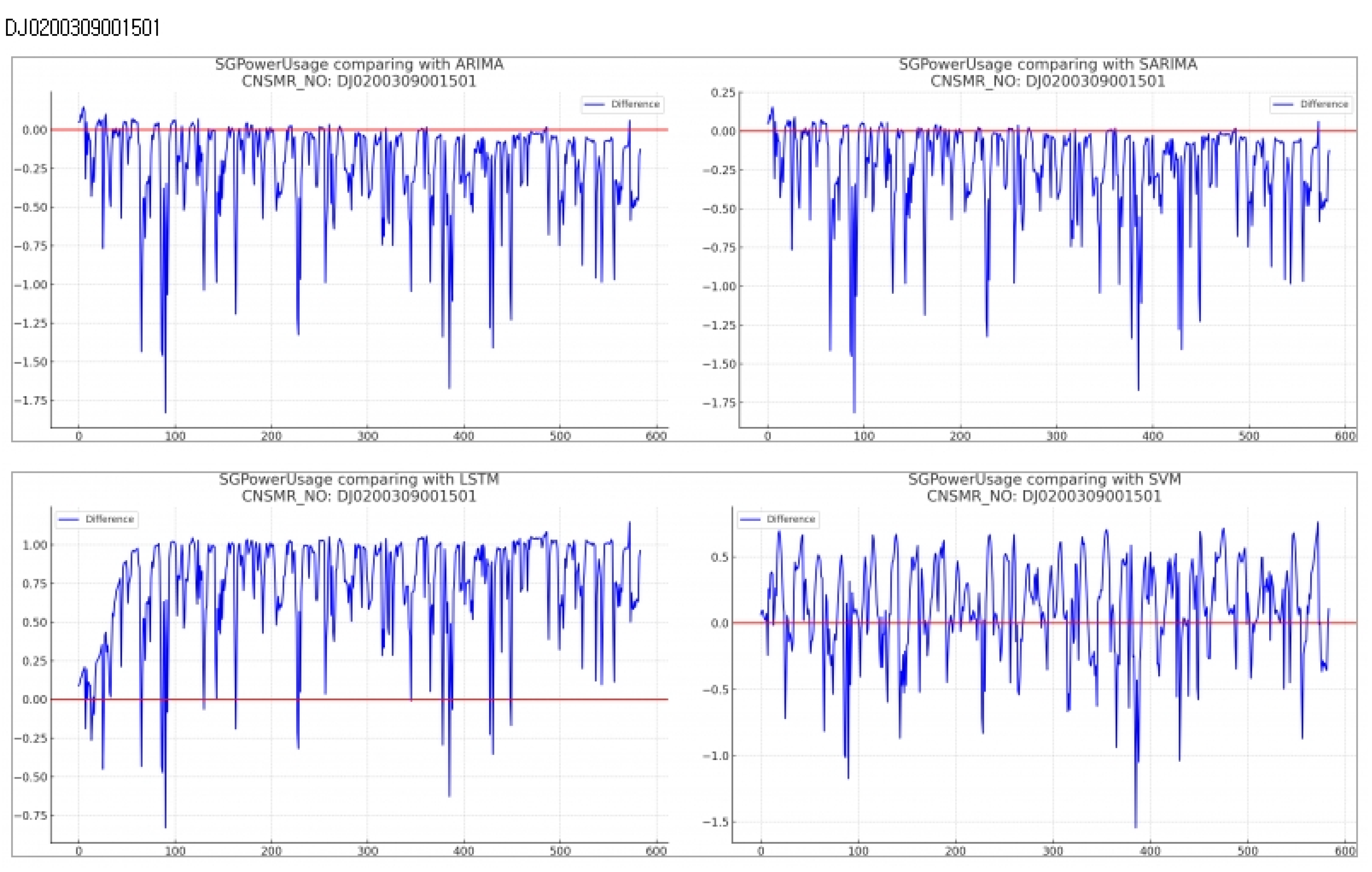
Figure 6.
Differences in SGPowerUsage Values Between Predictions and Actual Data in DJ0800133001204.
Figure 6.
Differences in SGPowerUsage Values Between Predictions and Actual Data in DJ0800133001204.
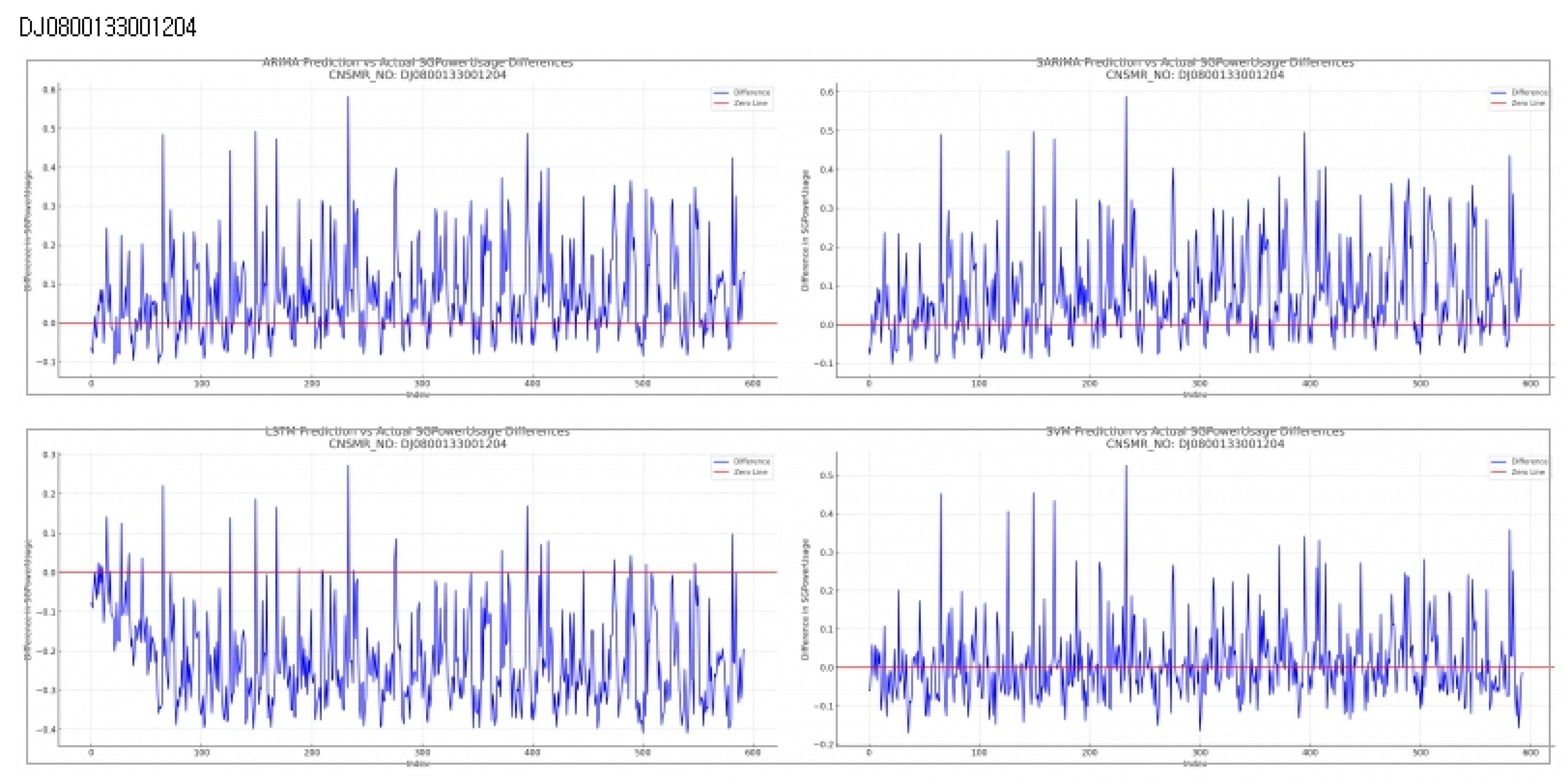
Figure 7.
Differences in SGPowerUsage Values Between Predictions and Actual Data in DJ1200215000404.
Figure 7.
Differences in SGPowerUsage Values Between Predictions and Actual Data in DJ1200215000404.
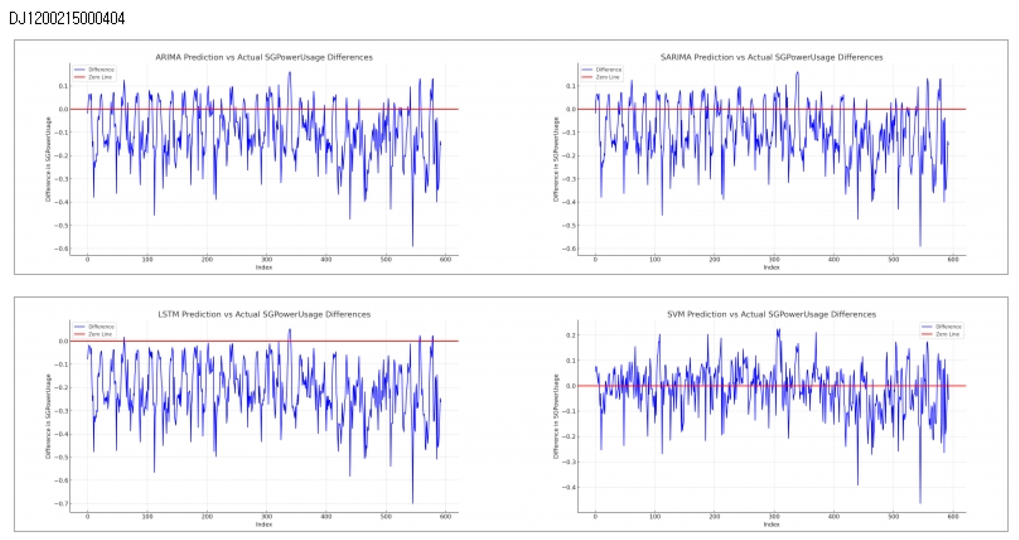
Figure 8.
Differences in SGPowerUsage Values Between Predictions and Actual Data in CB0100106000505.
Figure 8.
Differences in SGPowerUsage Values Between Predictions and Actual Data in CB0100106000505.
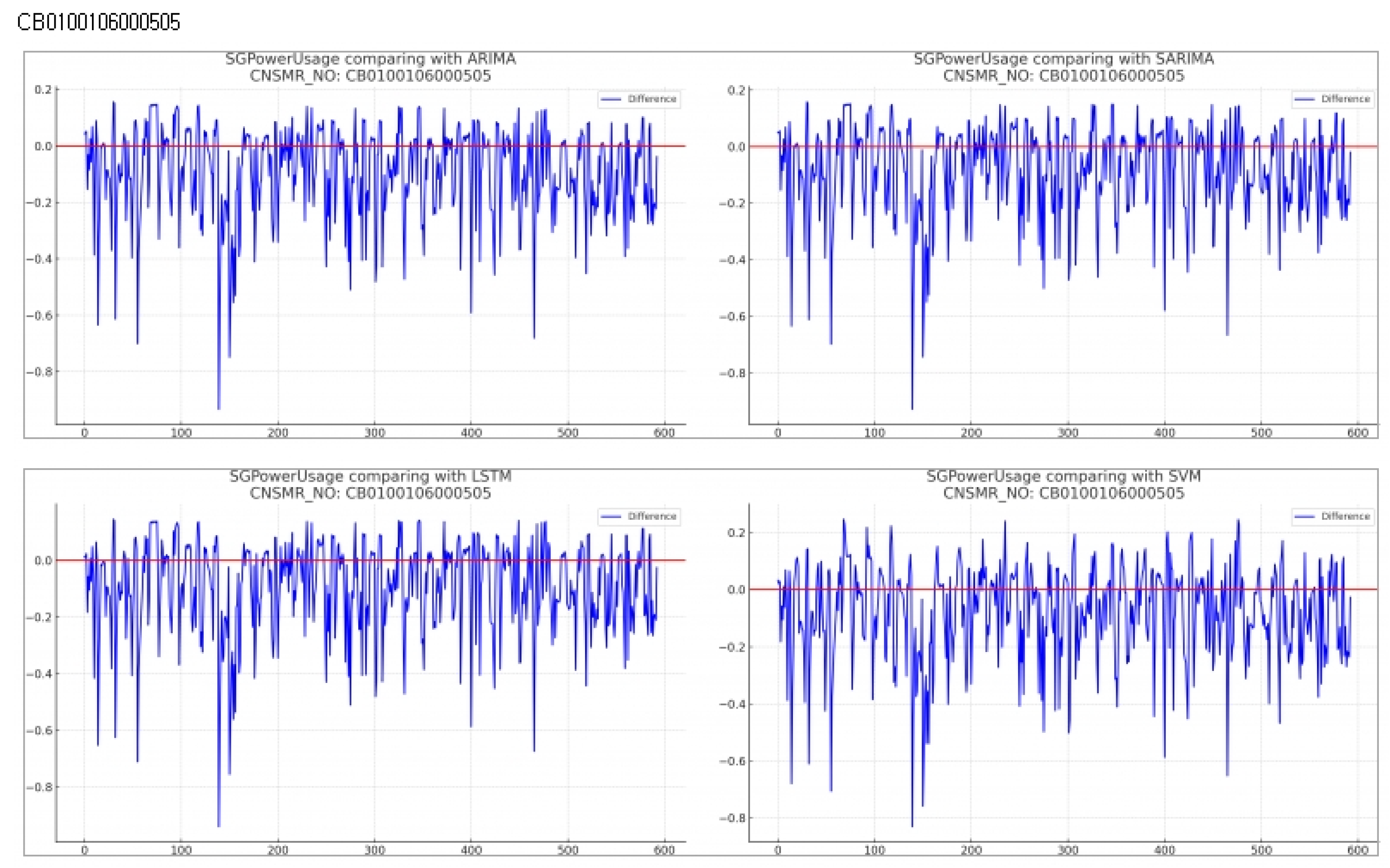
Figure 9.
Differences in SGPowerUsage Values Between Predictions and Actual Data in CN0100107001801.
Figure 9.
Differences in SGPowerUsage Values Between Predictions and Actual Data in CN0100107001801.
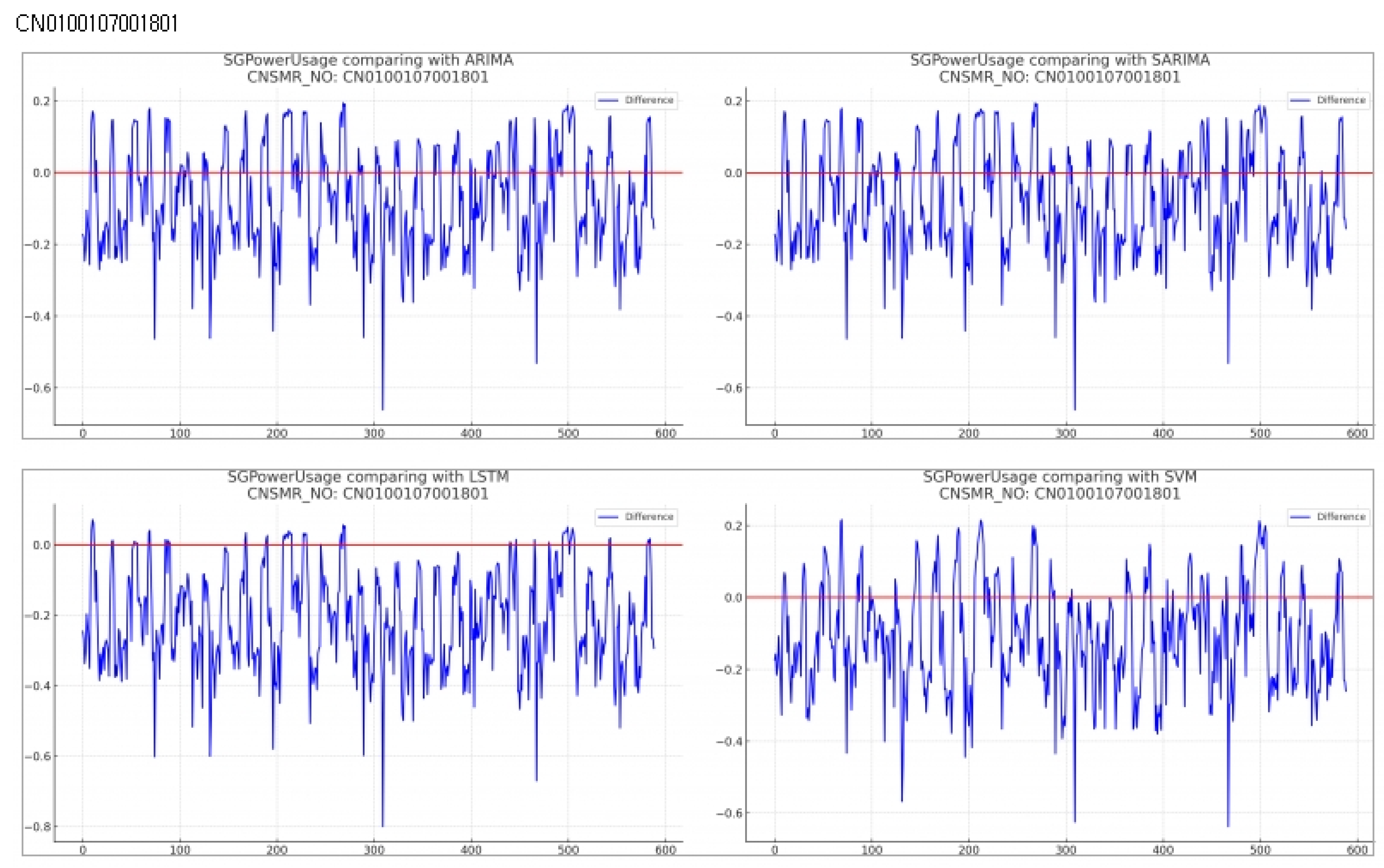
Figure 10.
Differences in SGPowerUsage Values Between Predictions and Actual Data in CN0200311001801.
Figure 10.
Differences in SGPowerUsage Values Between Predictions and Actual Data in CN0200311001801.
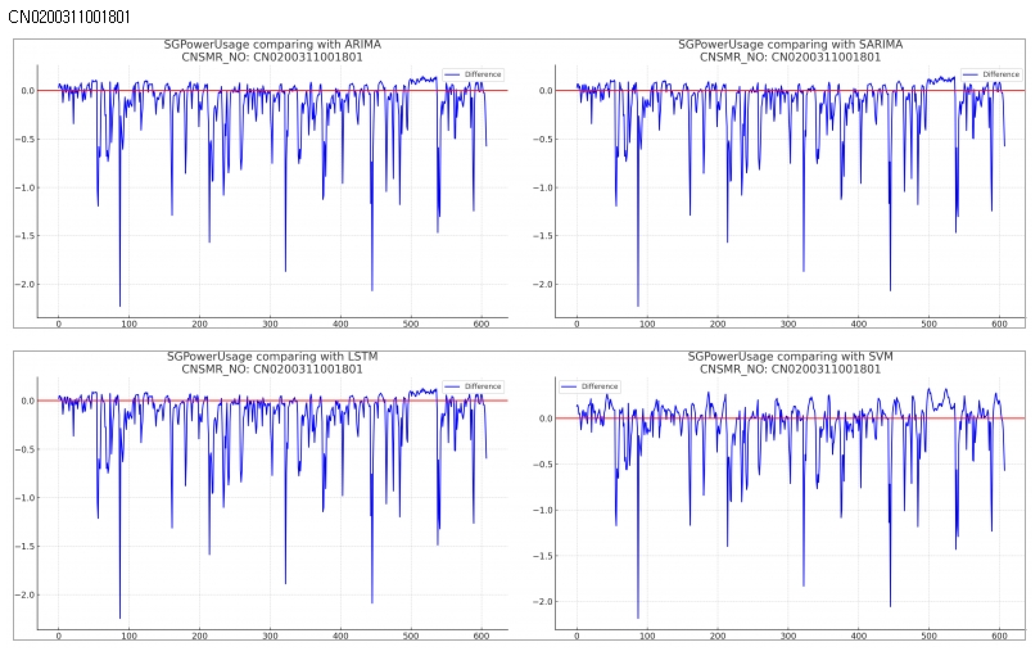
Figure 11.
Differences in SGPowerUsage Values Between Predictions and Actual Data in CN1100106000103.
Figure 11.
Differences in SGPowerUsage Values Between Predictions and Actual Data in CN1100106000103.
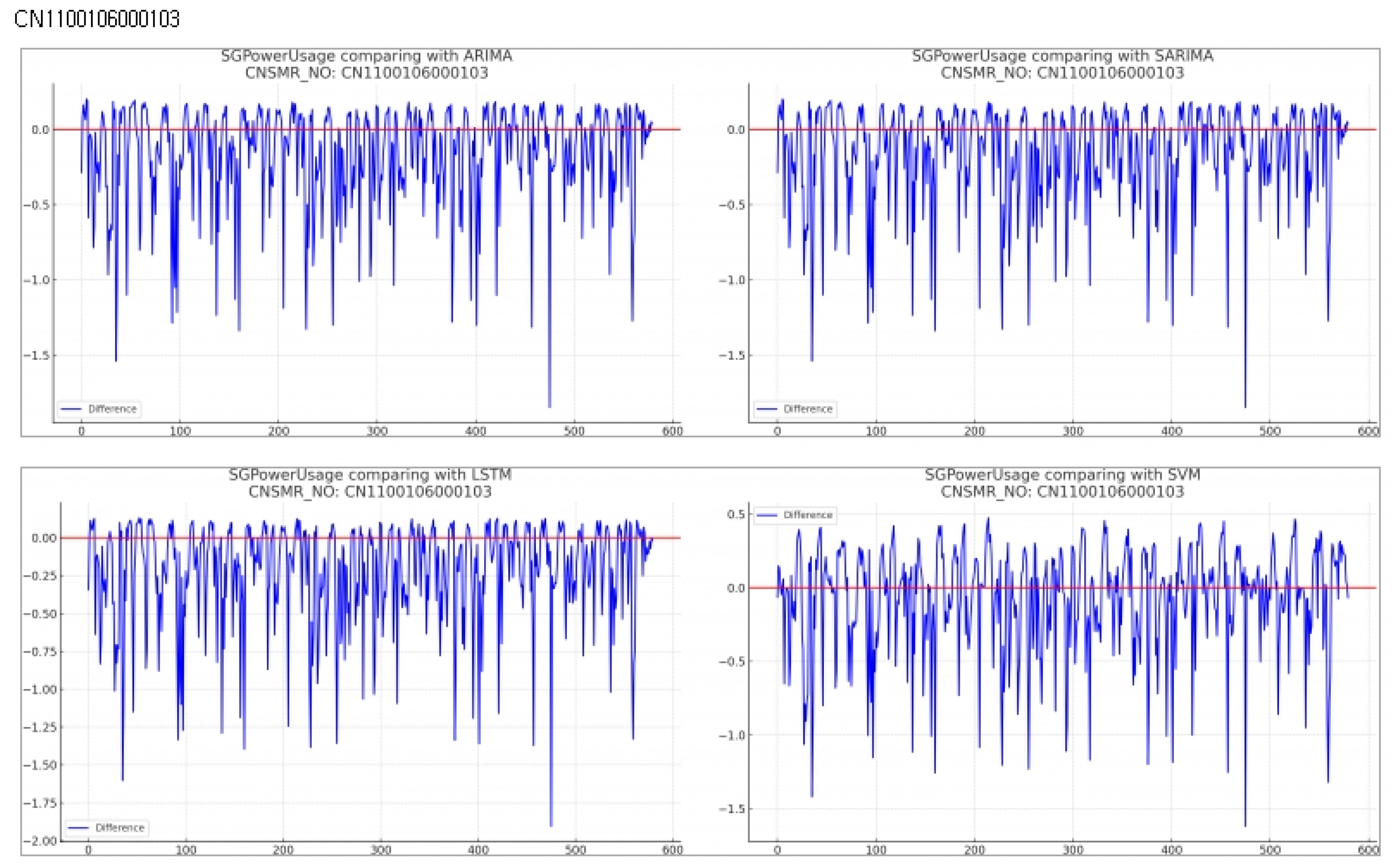
Figure 12.
Differences in SGPowerUsage Values Between Predictions and Actual Data in CN1600102001004.
Figure 12.
Differences in SGPowerUsage Values Between Predictions and Actual Data in CN1600102001004.
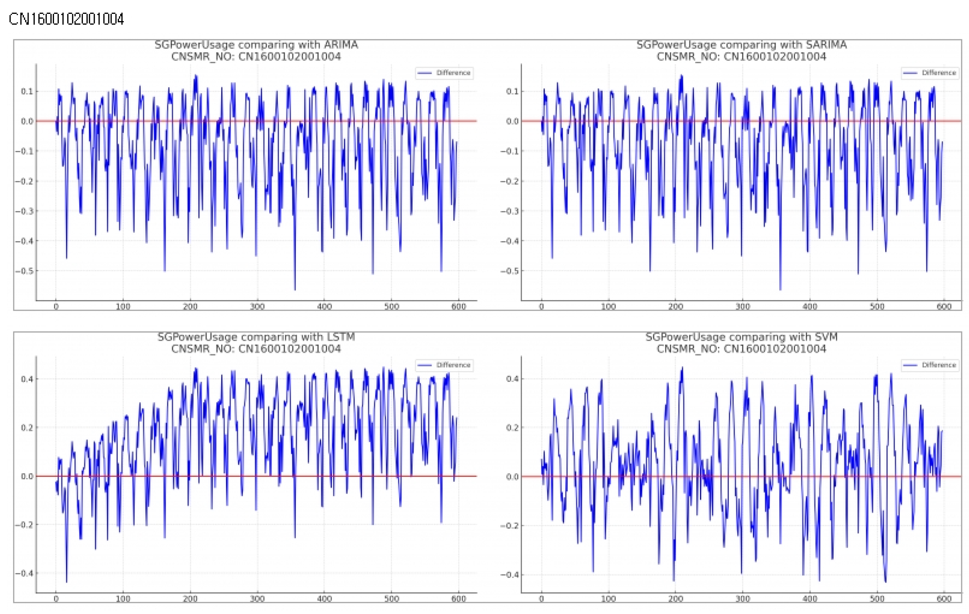
Figure 13.
Differences in SGPowerUsage Values Between Predictions and Actual Data in CN0500311000403.
Figure 13.
Differences in SGPowerUsage Values Between Predictions and Actual Data in CN0500311000403.
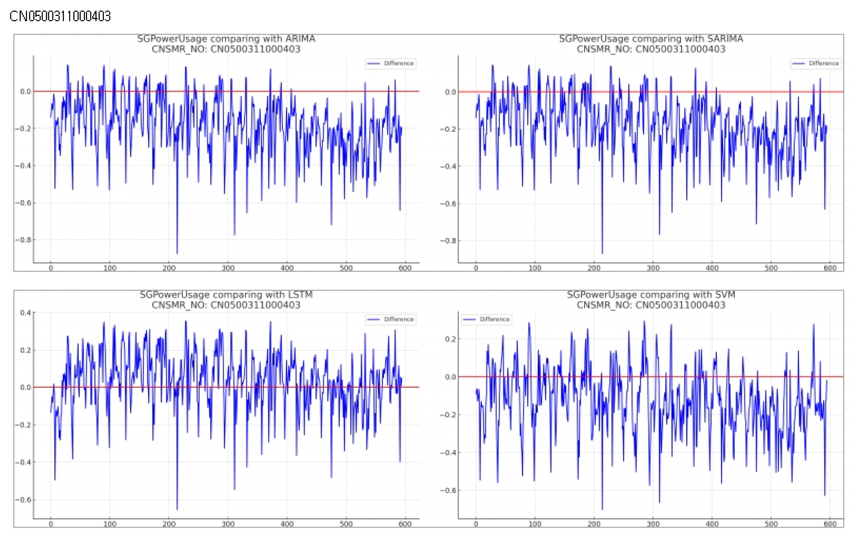
Figure 14.
Differences in SGPowerUsage Values Between Predictions and Actual Data in CN0700109000102.
Figure 14.
Differences in SGPowerUsage Values Between Predictions and Actual Data in CN0700109000102.
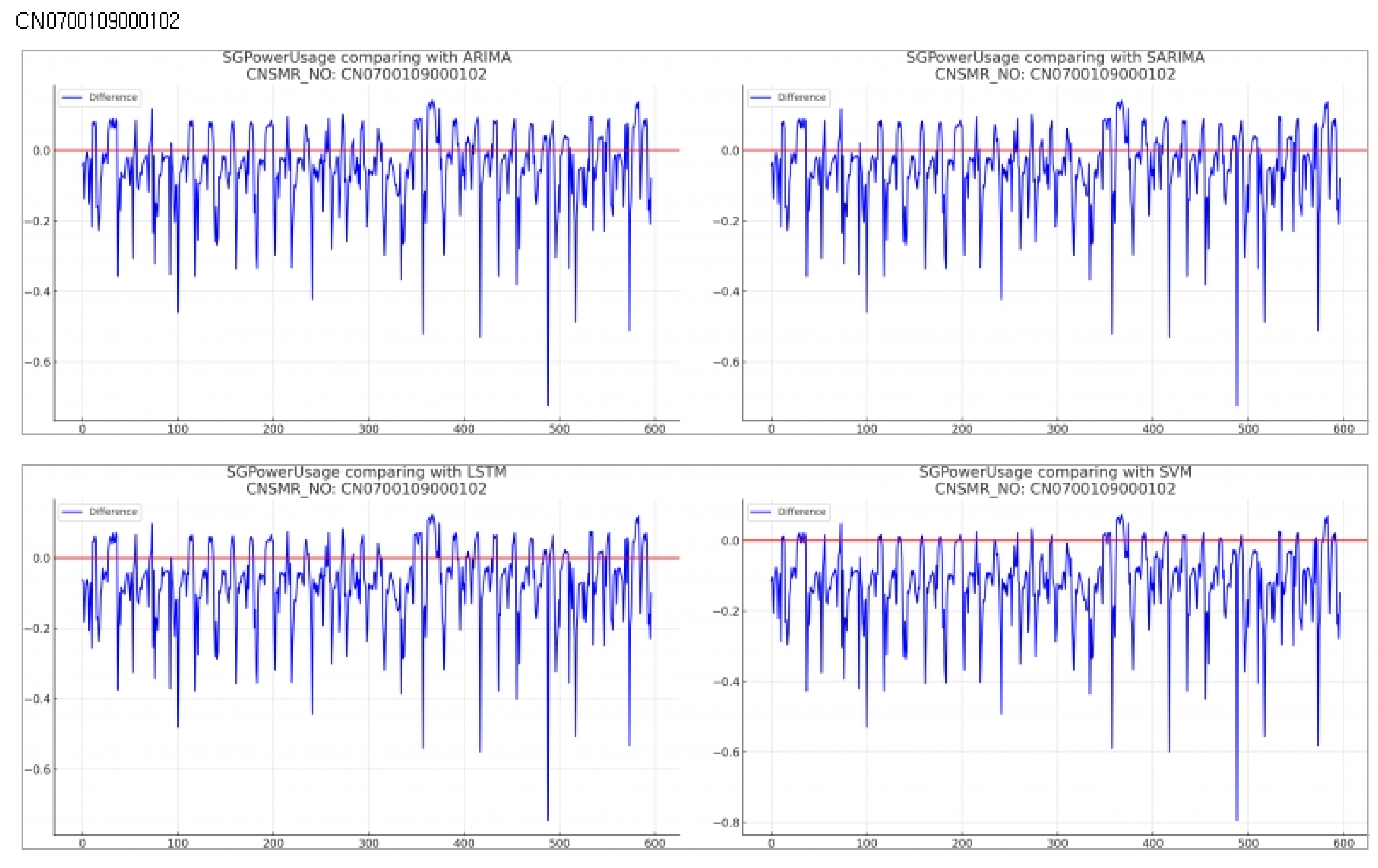
Figure 15.
Differences in SGPowerUsage Values Between Predictions and Actual Data.
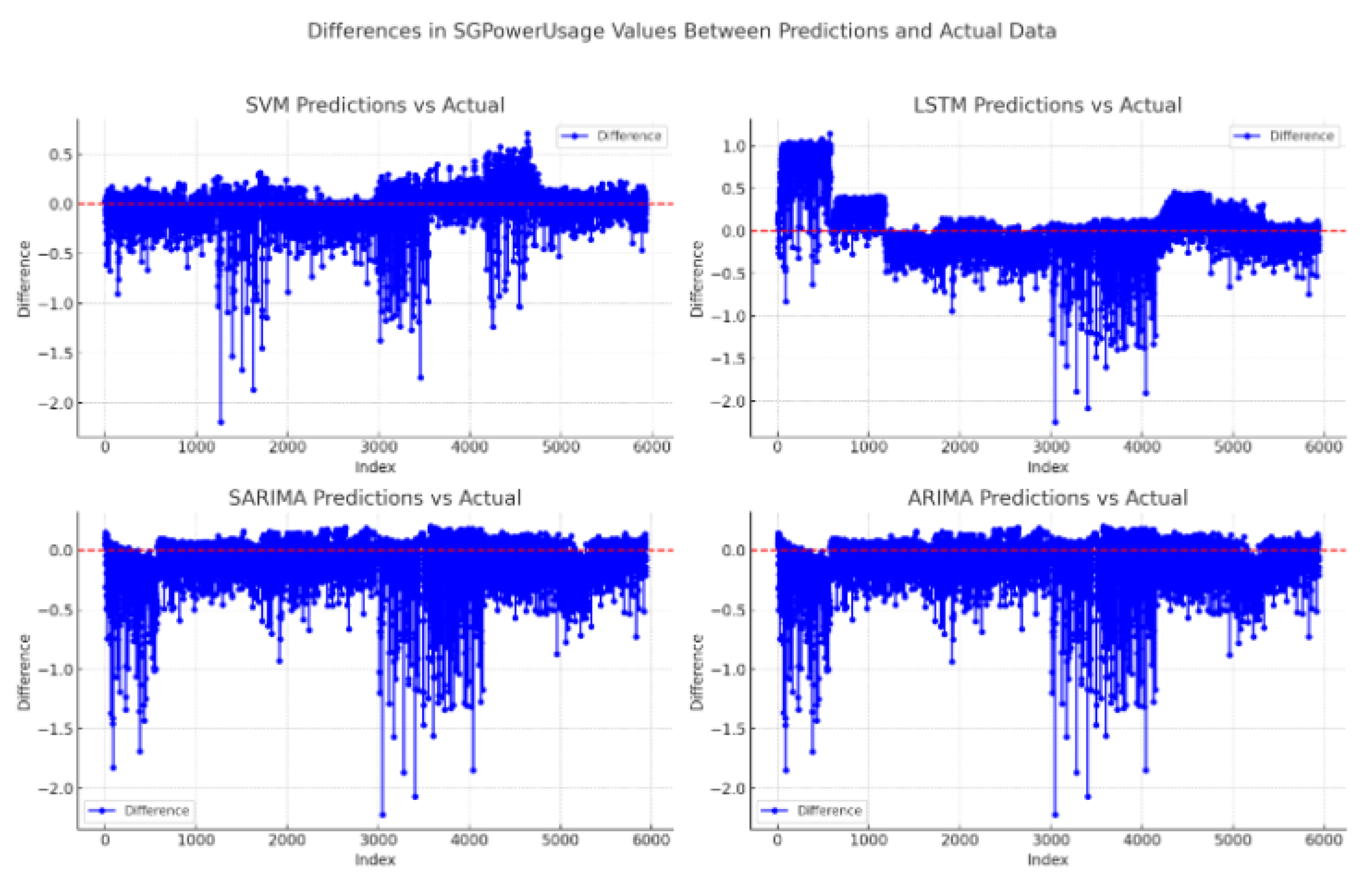

Table 1.
Data Specification for Time Series Analysis.
| English Name | Type | Length | Required | Identifier | Allowed Values | Example |
|---|---|---|---|---|---|---|
| TOC_NO | VARCHAR | 10 | Y | Y | Alphabet followed by numerical string | A000000001 |
| CNSMR_NO | VARCHAR | 20 | Y | Y | Random string | KB0100201000105 |
| LEGALDONG_CD | VARCHAR | 10 | Y | - | Numerical string | 2653010400 |
| MESURE_DE | VARCHAR | 8 | Y | Y | Post-2016 | 20190901 |
| MESURE_TM | VARCHAR | 2 | Y | Y | 00 23 | 14 |
Table 2.
Data Specification for Time Series Learning and Analysis.
| English Name | Type | Length | Required | Identifier | Example | |
|---|---|---|---|---|---|---|
| CNSMR_NO | VARCHAR | 20 | Y | Y | Random string | KB0100201000105 |
| LEGALDONG_CD | VARCHAR | 10 | Y | Number | 2653010400 | |
| MESURE_YEAR | VARCHAR | 4 | Y | Y | After 2016 | 2019 |
| MESURE_MT | VARCHAR | 2 | Y | Y | Number | 01 |
| MESURE_DTTM | VARCHAR | 2 | Y | Y | Number | 31 |
| MESURE_TM | VARCHAR | 2 | Y | Y | 00 23 | 14 |
| HLDY_AT | VARCHAR | 1 | Y | Y/N | Y | |
| SG_PWRER_USE_AM | NUMBER | 16 | Y | 0.0 9999999999.9999 | 0.345 |
Table 3.
Slope and intercept of forcasting data usgng ARIMA .
| CNSMR_NO | slope | intercept |
|---|---|---|
| CB0100106000505 | -0.001011758 | 20449.089 |
| CN0100107001801 | -9.081498547 | 0.313582719 |
| CN0200311001801 | 2.113108398 | -426.846467 |
| CN0500311000403 | -0.00149791 | 30274.77219 |
| CN0700109000102 | -5.007757692 | 1.181070942 |
| CN1100106000103 | -4.210372471 | 851.2864752 |
| CN1600102001004 | 8.987788029 | -17.93733817 |
| DJ0200309001501 | -0.005480365 | 110765.1287 |
| DJ0800133001204 | -0.000982641 | 19860.54595 |
| DJ1200215000404 | 5.463169948 | -110.0872162 |
Table 4.
Slope and intercept of forcasting data usgng SARIMA .
| CNSMR_NO | slope | intercept |
|---|---|---|
| CB0100106000505 | -0.000319073 | 6449.082179 |
| CN0100107001801 | 4.039360831 | -0.520846808 |
| CN0200311001801 | 2.280846442 | -460.7483028 |
| CN0500311000403 | -0.001123215 | 22701.73422 |
| CN0700109000102 | -5.009475262 | 1.1814181 |
| CN1100106000103 | -4.210357905 | 851.2835312 |
| CN1600102001004 | 8.987780947 | -17.93732388 |
| DJ0200309001501 | -0.005493802 | 111036.6921 |
| DJ0800133001204 | -0.001262886 | 25524.63396 |
| DJ1200215000404 | 5.463022253 | -110.0842315 |
Table 5.
Slope and intercept of forcasting data usgng LSTM .
| CNSMR_NO | slope | intercept |
|---|---|---|
| CB0100106000505 | 5.580297358 | -1127.623133 |
| CN0100107001801 | -0.000230448 | 4657.795984 |
| CN0200311001801 | -4.785285336 | 967.3830755 |
| CN0500311000403 | 0.001596365 | -32264.05829 |
| CN0700109000102 | 9.239923789 | -1867.352245 |
| CN1100106000103 | -2.525308407 | 510.6578743 |
| CN1600102001004 | 0.007655379 | -154724.0285 |
| DJ0200309001501 | 0.007879234 | -159247.6266 |
| DJ0800133001204 | 0.003431755 | -69359.46656 |
| DJ1200215000404 | -0.000103266 | 2087.36154 |
Table 6.
Slope and intercept of forcasting data usgng SVM
| CNSMR_NO | slope | intercept |
|---|---|---|
| CB0100106000505 | 8.233022059 | 0.2380441 |
| CN0100107001801 | 8.233022059 | 0.262161614 |
| CN0200311001801 | -7.409719853 | 0.309545457 |
| CN0500311000403 | 1.646604412 | 0.258864742 |
| CN0700109000102 | 0 | 0.1 |
| CN1100106000103 | -3.293208824 | 0.407003965 |
| CN1600102001004 | 2.140585735 | 0.357806174 |
| DJ0200309001501 | 3.293208824 | 0.651065178 |
| DJ0800133001204 | -6.586417647 | 0.238392017 |
| DJ1200215000404 | 1.317283529 | 0.424890753 |
Table 7.
DJ0200309001501 Performance evaluation.
| Consumer Number(CNSMR_NO) | DJ0200309001501 | ||
|---|---|---|---|
| Algorithm | MSE | MAE | RMSE |
| ARIMA | 0.144 | 0.253 | 0.38 |
| SARIMA | 0.143 | 0.25 | 0.378 |
| LSTM | 0.675 | 0.777 | 0.821 |
| SVM | 0.076 | 0.198 | 0.276 |
Table 8.
DJ0800133001204 Performance evaluation.
| Consumer Number(CNSMR_NO) | DJ0800133001204 | ||
|---|---|---|---|
| Algorithm | MSE | MAE | RMSE |
| ARIMA | 0.018 | 0.094 | 0.134 |
| SARIMA | 0.019 | 0.097 | 0.138 |
| LSTM | 0.065 | 0.232 | 0.255 |
| SVM | 0.009 | 0.068 | 0.097 |
Table 9.
DJ1200215000404 Performance evaluation.
| Consumer Number(CNSMR_NO) | DJ1200215000404 | ||
|---|---|---|---|
| Algorithm | MSE | MAE | RMSE |
| ARIMA | 0.024 | 0.124 | 0.154 |
| SARIMA | 0.024 | 0.124 | 0.154 |
| LSTM | 0.057 | 0.208 | 0.238 |
| SVM | 0.009 | 0.071 | 0.093 |
Table 10.
CB0100106000505 Performance evaluation.
| Consumer Number(CNSMR_NO) | CB0100106000505 | ||
|---|---|---|---|
| Algorithm | MSE | MAE | RMSE |
| ARIMA | 0.034 | 0.133 | 0.185 |
| SARIMA | 0.032 | 0.130 | 0.179 |
| LSTM | 0.034 | 0.132 | 0.184 |
| SVM | 0.029 | 0.117 | 0.169 |
Table 11.
CN0100107001801 Performance evaluation.
| Consumer Number(CNSMR_NO) | CN0100107001801 | ||
|---|---|---|---|
| Algorithm | MSE | MAE | RMSE |
| ARIMA | 0.026 | 0.132 | 0.160 |
| SARIMA | 0.025 | 0.132 | 0.160 |
| LSTM | 0.065 | 0.216 | 0.254 |
| SVM | 0.026 | 0.132 | 0.161 |
Table 12.
CN0200311001801 Performance evaluation.
| Consumer Number(CNSMR_NO) | CN0200311001801 | ||
|---|---|---|---|
| Algorithm | MSE | MAE | RMSE |
| ARIMA | 0.111 | 0.178 | 0.333 |
| SARIMA | 0.111 | 0.178 | 0.333 |
| LSTM | 0.117 | 0.185 | 0.342 |
| SVM | 0.087 | 0.161 | 0.295 |
Table 13.
CN1100106000103 Performance evaluation.
| Consumer Number(CNSMR_NO) | CN1100106000103 | ||
|---|---|---|---|
| Algorithm | MSE | MAE | RMSE |
| ARIMA | 0.136 | 0.242 | 0.368 |
| SARIMA | 0.136 | 0.242 | 0.368 |
| LSTM | 0.156 | 0.255 | 0.395 |
| SVM | 0.096 | 0.187 | 0.310 |
Table 14.
CN1600102001004 Performance evaluation.
| Consumer Number(CNSMR_NO) | CN1600102001004 | ||
|---|---|---|---|
| Algorithm | MSE | MAE | RMSE |
| ARIMA | 0.026 | 0.122 | 0.162 |
| SARIMA | 0.026 | 0.122 | 0.162 |
| LSTM | 0.063 | 0.216 | 0.251 |
| SVM | 0.011 | 0.082 | 0.106 |
Table 15.
CN0500311000403 Performance evaluation.
| Consumer Number(CNSMR_NO) | CN0500311000403 | ||
|---|---|---|---|
| Algorithm | MSE | MAE | RMSE |
| ARIMA | 0.057 | 0.190 | 0.232 |
| SARIMA | 0.054 | 0.190 | 0.232 |
| LSTM | 0.024 | 0.122 | 0.156 |
| SVM | 0.034 | 0.147 | 0.184 |
Table 16.
CN0700109000102 Performance evaluation.
| Consumer Number(CNSMR_NO) | CN0700109000102 | ||
|---|---|---|---|
| Algorithm | MSE | MAE | RMSE |
| ARIMA | 0.014 | 0.085 | 0.120 |
| SARIMA | 0.014 | 0.085 | 0.120 |
| LSTM | 0.017 | 0.095 | 0.130 |
| SVM | 0.026 | 0.124 | 0.161 |
Disclaimer/Publisher’s Note: The statements, opinions and data contained in all publications are solely those of the individual author(s) and contributor(s) and not of MDPI and/or the editor(s). MDPI and/or the editor(s) disclaim responsibility for any injury to people or property resulting from any ideas, methods, instructions or products referred to in the content. |
© 2024 by the authors. Licensee MDPI, Basel, Switzerland. This article is an open access article distributed under the terms and conditions of the Creative Commons Attribution (CC BY) license (http://creativecommons.org/licenses/by/4.0/).
Copyright: This open access article is published under a Creative Commons CC BY 4.0 license, which permit the free download, distribution, and reuse, provided that the author and preprint are cited in any reuse.


