LSTM‐Based Time Series Detection of Abnormal Electricity Usage in Smart Meters

Jingyi Huang; Yujuan Qiu

doi:10.20944/preprints202506.1404.v1

Submitted:

13 June 2025

Posted:

17 June 2025

You are already at the latest version

Abstract

In order to improve the accuracy and real-time performance of detecting abnormal behavior of smart meters, a time series prediction model based on Long Short-Term Memory (LSTM) is constructed, combining the sliding window mechanism and the residual dynamic thresholding strategy to realize the determination of abnormal behavior. The study covers data preprocessing, model structure design, system deployment, and visualization feedback, and optimizes the training performance by introducing Early Stopping, Dropout and learning rate adjustment. Comparison experiments are carried out based on real residential electricity consumption data, and the analysis shows that the LSTM model is better than traditional methods such as ARIMA, SVR and GRU in terms of prediction error and recognition accuracy, and it has strong sequence modeling capability and anomaly recognition stability.

Keywords:

smart meter

;

anomaly detection

;

LSTM

;

time series

Subject:

Computer Science and Mathematics - Artificial Intelligence and Machine Learning

I. Introduction

With the continuous complexity of urban power load structure and the highly diversified behavior of residents' power usage, the traditional rule-driven abnormal power usage detection methods gradually show the problem of insufficient adaptability in terms of timeliness and accuracy. As a new type of power distribution terminal, the smart meter's high-frequency data collection capability provides rich time series information support for user behavior modeling and abnormal state identification [1]. Mining the implied power usage patterns from the huge multi-dimensional time series and realize high-precision and low-latency intelligent recognition has become a key challenge in power information management. Oriented to this problem, the introduction of deep models with sequence learning capability to optimize the anomaly detection method has important engineering application value and theoretical exploration significance.

II. LSTM-Based Model Design for Abnormal Power Usage Detection

A. Data Preprocessing Methods

The data preprocessing stage mainly includes missing value filling, outlier identification and statute, normalization processing and time window reconstruction. Firstly, the original smart meter readings with an acquisition period of 15 minutes are calibrated for continuity, and the linear interpolation method is used to repair the intermittent data with a proportion of less than 3% to avoid the destruction of the temporal structure. Secondly, the non-systematic perturbation values in the training samples are removed by the local outlier factor (LOF) method to enhance the model robustness [2]. In terms of numerical statute, Min-Max normalization is chosen to map all electricity consumption data to the interval [0,1], which unifies the feature scale and satisfies the input characteristics of the LSTM activation function. In order to enhance the sequence learning ability of the model, the original sequence is reconstructed based on the sliding window mechanism into a sequence of the form (Xt,Xt+1,..., Xt+n) input segments, where the window length n is taken as 96, covering the complete 24-hour electricity cycle.

B. LSTM Model Structure Design

The model structure utilizes a standard multi-layer LSTM stacking approach to capture long-term dependency patterns in smart meter electricity consumption data. The input layer receives time-series window data shaped like [96,1], representing 24 consecutive hours of univariate electricity consumption records. The first LSTM layer contains 64 cells and employs a tanh activation function to enhance nonlinear fitting, and the output sequence is passed to the second LSTM layer (32 cells) to further compress the time-series feature dimensions and enhance sensitivity to key behavioral changes. Subsequently mapped through a fully connected layer, the output is a single-step prediction, which is compared with the actual value to achieve residual modeling [3]. The network employs mean square error (MSE) as the loss function and uses the Adam optimizer to control the learning rate with an initial value of 0.001. The overall structure is shown in Figure 1, where the number of neural units and type of activation function in each layer are indicated to clarify the data flow paths, which helps in the visual understanding and implementation of the model structure.

C. Anomaly Detection Threshold Determination

After completing the LSTM prediction, the system needs to construct an anomaly identification mechanism based on the residuals between the predicted and actual values. In order to enhance the adaptability of the model to diversified user behaviors, this study adopts the statistical threshold method to analyze and model the residual sequences. The specific method is to calculate the mean value μ and standard deviation σ of all predicted residuals in the training set, and set μ + kσ as the upper threshold, where k reflects the sensitivity adjustment factor, which is usually taken as the value of 2.0, 2.5, 3.0, etc. [4]. Table 1 lists the threshold ranges and corresponding coverage rates under different values of k, which facilitates the flexible selection according to the false alarm control objective in practical applications, and improves the stability and reliability of the system [5]. This mechanism can achieve stable identification of abnormal behaviors, while retaining a certain degree of elasticity to avoid misjudgment triggered by fluctuations in electricity consumption, thus supporting the high fault tolerance and generalization ability of the model in practical deployment [6].

D. Model Optimization Strategy

To enhance the LSTM model's training efficiency and generalization ability in anomaly detection, a multi-dimensional optimization strategy is employed. The Early Stopping mechanism halts training when the validation set loss does not decrease significantly for 5 consecutive epochs, preventing overfitting. L2 regularization is applied to the model weights with a coefficient of 0.001 to avoid parameter explosion. Dropout is used to increase robustness, with deactivation probabilities of 0.2 and 0.3 applied after the first and second LSTM layers, respectively, reducing feature dependency. A dynamic learning rate adjustment mechanism is introduced to reduce the learning rate from 0.001 by a factor of 0.1 based on validation error changes. Table 2 shows the parameters and triggering mechanisms of these optimization methods, creating a structured training optimization system for stable and scalable LSTM model training in power consumption anomaly detection [7].

III. Algorithm Implementation and System Design

A. System Architecture Design

The system uses a layered architecture with four core modules: data acquisition, data preprocessing, model inference, and result service. The data layer collects electricity consumption records via Modbus-TCP protocol and uploads them to the cloud after edge node cleaning. The middle layer, built with Python, manages data preprocessing and model loading to ensure compatibility with LSTM input requirements. The model inference layer deploys the optimized LSTM network in a TensorRT environment via ONNX format for improved performance. Results are then sent to the front-end visualization system through a Web API interface. Figure 2 illustrates the functional modules and data pathways, ensuring algorithm integrity and efficient deployment.

B. Data Acquisition and Storage Module

The front-end of the system is deployed in the smart meter devices in the distribution boxes of residential buildings, supporting 15-minute/point high-frequency energy consumption data acquisition, which is transmitted to the edge data acquisition unit in real time using Modbus-TCP protocol. The acquisition module realizes fault tolerance to network fluctuations through the data buffering mechanism, and at the same time encapsulates multi-dimensional measurement indexes such as current, voltage, active power, etc. in JSON structure [7]. The collected data is first stored in the local Redis cache to improve real-time performance, and then periodically synchronized to the back-end MongoDB database for structured query and time series analysis. To meet the demand for long-term data accumulation, the system enables automatic slicing and archiving mechanism to realize monthly compression and hot/cold tiered storage of historical data. Table 3 summarizes the core data fields, collection cycles and their data types, providing standardized support for subsequent model input and system performance evaluation [8].

C. Anomaly Detection Module Implementation

The anomaly detection module is deployed in the cloud-based inference layer, using optimized LSTM models encapsulated in ONNX format and loaded into the TensorRT inference engine for low-latency response. The model takes a preprocessed sliding time window sequence with a fixed dimension of [96,1], representing 24 hours of electricity consumption data. The system processes the input, performs forward prediction, and calculates residuals by comparing the output with real-time meter readings [9]. Anomalies are detected based on a dynamic threshold. The detection process is encapsulated as a RESTful interface via Flask, supporting batch uploads and asynchronous result returns for fast integration with the front-end visualization system. Valid anomalies trigger structured alarm logs, which are written to a Kafka queue for alarm service subscription. Figure 3 shows the processing flow and interaction path of the anomaly detection module in the data flow and service logic.

D. Results Visualization Design

The front-end visualization interface is built using the Vue framework and ECharts for graphical rendering, enabling real-time presentation and interactive feedback of anomaly detection results. The back-end sends standardized JSON data to the front-end via RESTful API, including timestamps, predicted values, actual values, and anomaly markers for efficient and dynamic visualization updates. The interface features a multi-chart layout, with the top line graph comparing predicted and actual values, and the bottom heat map showing anomaly time periods and frequencies. Clicking on an anomaly displays detailed power consumption records and error analysis reports for quick tracking by maintenance staff. Figure 4 illustrates the interface structure and interactive logic, ensuring effective integration of detection results and user interaction.

IV. Experimental Results and Analysis

A. Experimental Environment and Data Set

Experiments were conducted on Ubuntu 20.04 with an Intel Xeon Gold 5218 processor (2.3GHz, 16 cores), 128GB RAM, and an NVIDIA RTX A5000 GPU (24GB memory) to ensure efficient LSTM model training on large-scale time series and parallel inference. The deep learning framework used was PyTorch 1.13.1, with model deployment in ONNX format and accelerated inference via TensorRT 8.6. The experimental data came from smart meter records of 512 residential users in a provincial capital city in 2022, spanning 9 months. Data was collected every 15 minutes, with 96 data points per day, including timestamp, voltage, current, active power, and reactive power, as detailed in Table 3. The preprocessed training and validation sets contain 115,200 and 28,800 sliding window sequences, respectively, each of dimension [96,1]. To ensure data representativeness, samples from various seasons and holidays were included. Figure 5 shows the heat map of electricity consumption for a typical user over three days, illustrating periodic behavioral changes and supporting the model prediction task [10].

B. Design of Evaluation Indicators

In order to comprehensively assess the accuracy and robustness of the LSTM model in the smart meter anomaly detection task, the evaluation system needs to be constructed at two levels: prediction accuracy and anomaly identification effectiveness. In terms of prediction accuracy, Mean Squared Error (MSE) and Mean Absolute Error (MAE) are used to measure the fitting ability of the model within a sliding time window, which are defined as [10]:

M A E = \frac{1}{n} \sum_{i = 1}^{n} |y_{i} - {\hat{y}}_{i}|, M S E = \frac{1}{n} \sum_{i = 1}^{n} {(y_{i} - {\hat{y}}_{i})}^{2}

where yi is the true value, y^i is the model predicted value, and n is the number of samples. This class of metrics can quantify the fitting ability of the LSTM model to the regular electricity use behavior, which serves as the basic support for the residual threshold judgment. For the anomaly recognition performance, Precision, Recall and F1-score are used to form a performance triad to reflect the model's recognition ability under different types of anomalies, as defined below:

\Pr e c i s i o n = \frac{T P}{T P + F P}, Re c a l l = \frac{T P}{T P + F N}, F 1 = \frac{2 \times \Pr e c i s i o n \times Re c a l l}{\Pr e c i s i o n + Re c a l l}

Where TP is the number of samples that are truly abnormal and judged to be abnormal, FP is the number of normal samples that are misjudged as abnormal, and FN is the number of abnormal samples that are misjudged as normal.

C. Comparative Analysis of Model Performance

To verify the superior performance of the LSTM model in detecting abnormal electricity consumption, the experiment compares LSTM with three other sequence modeling algorithms—ARIMA, Support Vector Regression (SVR), and a single-layer GRU model—using the same dataset and evaluation metrics. Figure 6 shows the forecast trend curves of the four models on typical customer data, with LSTM maintaining higher accuracy during periods of intense load fluctuations. Table 4 presents the MSE, MAE, Precision, Recall, and F1-score results for each model. LSTM achieves the lowest MSE (0.0084) and MAE (0.065), outperforming ARIMA (MSE 0.0241) and SVR (MSE 0.0176). In anomaly detection, LSTM's F1-score of 0.931 is significantly higher than GRU (0.894) and SVR (0.852), demonstrating its stronger ability to discriminate in complex consumption patterns. Additionally, LSTM's Recall value of 0.949 shows its ability to identify most anomalies while maintaining high Precision, minimizing false alarms. Figure 6 visualizes the model's response to abnormal intervals, highlighting LSTM’s advantage in modeling long sequence dependencies and controlling stable error bounds. Overall, the results confirm that LSTM has superior prediction and detection capabilities for residential electricity data, which often exhibits nonlinear, periodic, and bursty behavior.

V. Conclusions

The LSTM model shows excellent time-dependent modeling ability in processing smart meter power consumption sequences, which can effectively capture the periodic and sudden behavioral changes of users and realize the accurate identification of abnormal power consumption events. Combining the multilayer network structure, dynamic residual thresholding strategy and edge cloud cooperative system, an end-to-end detection system with high robustness and practicality is constructed. Compared with the traditional methods, the prediction accuracy and anomaly identification ability are significantly improved. However, the generalization ability of the model for different seasons, holidays and other complex electricity consumption patterns is still uncertain, and the use of correlation between multi-dimensional indicators is still relatively single. In the future, multivariate LSTM or attention mechanism can be introduced to further strengthen the model expression ability, and explore the fusion strategy of adaptive thresholding and user behavioral portrait, so as to promote the landing and evolution of the intelligent power monitoring system in a wider range of scenarios.

References

Takiddin A, Ismail M, Zafar U, et al. Deep autoencoder-based anomaly detection of electricity theft cyberattacks in smart grids[J]. IEEE Systems Journal, 2022, 16(3): 4106-4117. [CrossRef]
Śmiałkowski T, Czyżewski A. Detection of anomalies in the operation of a road lighting system based on data from smart electricity meters[J]. Energies, 2022, 15(24): 9438.
Munawar S, Asif M, Kabir B, et al. Electricity theft detection in smart meters using a hybrid Bi-directional GRU Bi-directional LSTM model[C]//Complex, Intelligent and Software Intensive Systems: Proceedings of the 15th International Conference on Complex, Intelligent and Software Intensive Systems (CISIS-2021). Springer International Publishing, 2021: 297-308.
Ahir R K, Chakraborty B. Pattern-based and context-aware electricity theft detection in smart grid[J]. Sustainable Energy, Grids and Networks, 2022, 32: 100833.
Otuoze A O, Mustafa M W, Sultana U, et al. Detection and confirmation of electricity thefts in Advanced Metering Infrastructure by Long Short-Term Memory and fuzzy inference system models[J]. Nigerian Journal of Technological Development, 2024, 21(1): 112-130. [CrossRef]
Zhou M, Musilek P. Real-time anomaly detection in distribution grids using long short term memory network[C]//2021 IEEE Electrical Power and Energy Conference (EPEC). IEEE, 2021: 208-213.
Lee S, Jin H, Nengroo S H, et al. Smart metering system capable of anomaly detection by bi-directional LSTM autoencoder[C]//2022 IEEE International Conference on Consumer Electronics (ICCE). IEEE, 2022: 1-6.
Eddin M E, Albaseer A, Abdallah M, et al. Fine-tuned RNN-based detector for electricity theft attacks in smart grid generation domain[J]. IEEE Open Journal of the Industrial Electronics Society, 2022, 3: 733-750.
Pamir, Javaid N, Javaid S, et al. Synthetic theft attacks and long short term memory-based preprocessing for electricity theft detection using gated recurrent unit[J]. Energies, 2022, 15(8): 2778. [CrossRef]
Zihan W, Enze S, Can W, et al. LSTM-Based Method for Electric Consumption Outlier Detection[C]//2021 IEEE Sustainable Power and Energy Conference (iSPEC). IEEE, 2021: 3955-3959.

Figure 1. Structure of LSTM anomaly detection model.

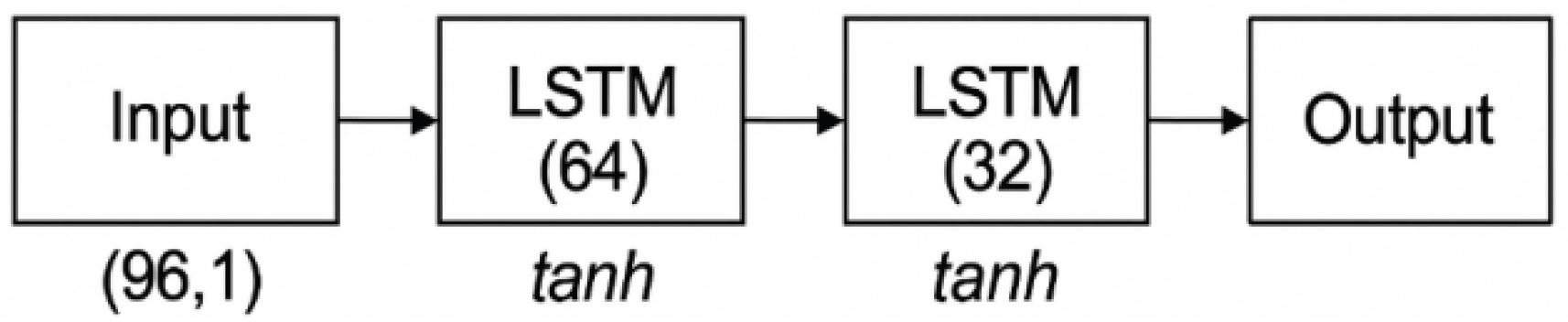
Figure 2. Architecture of LSTM power usage anomaly detection system.

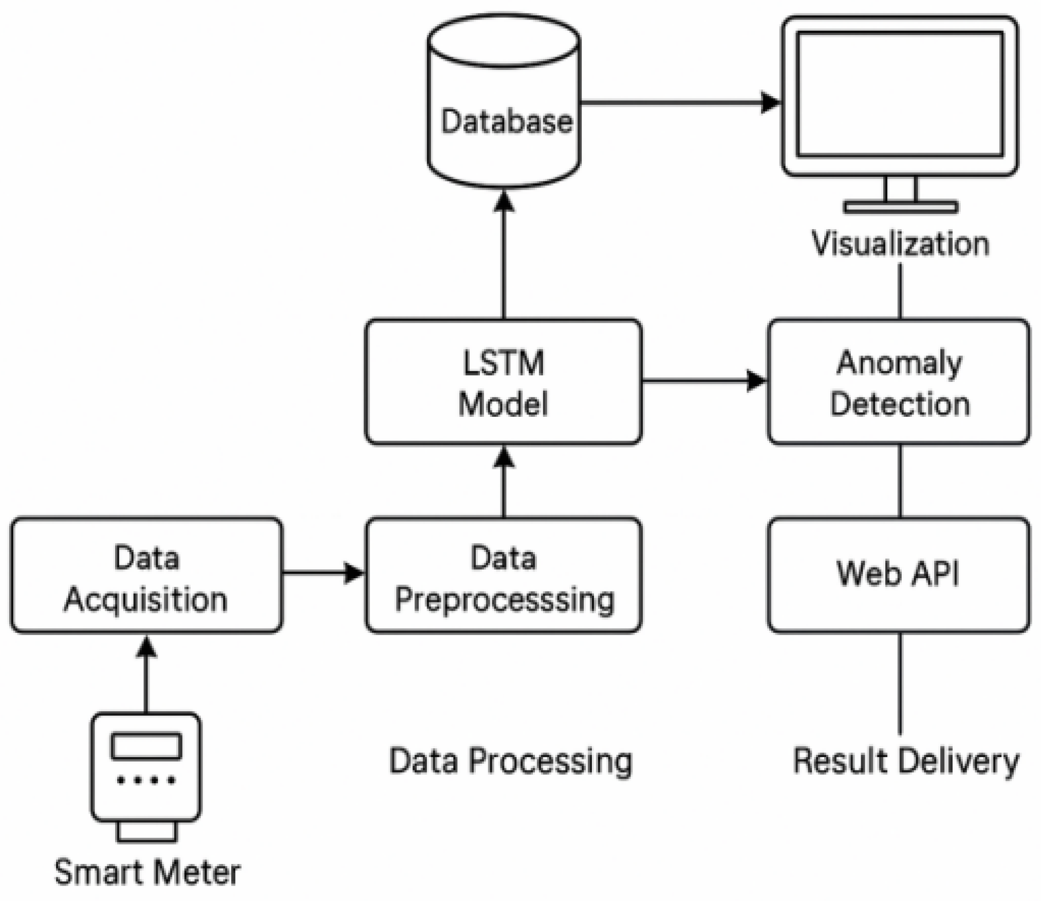
Figure 3. Logic flowchart of LSTM anomaly detection module.

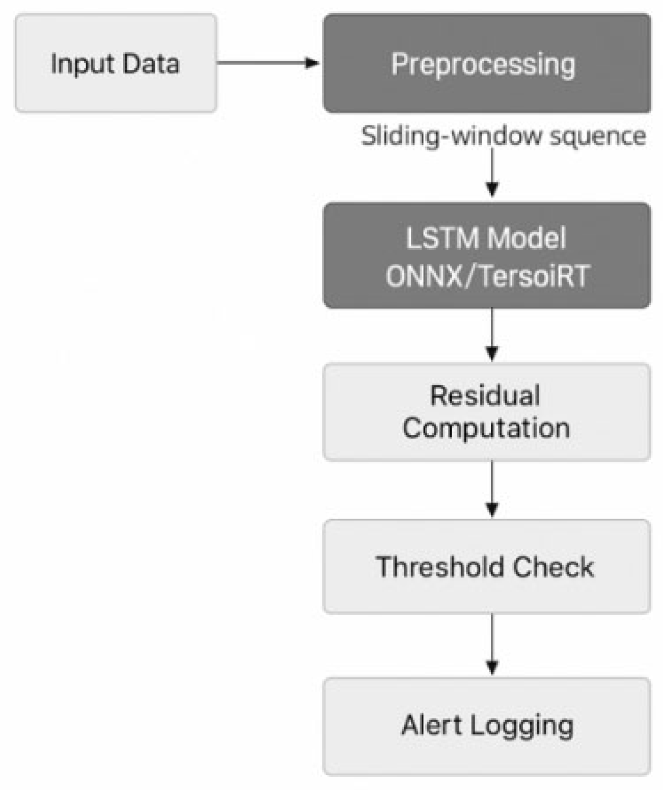
Figure 4. Structure of the interface for visualizing the results of power consumption anomaly detection.

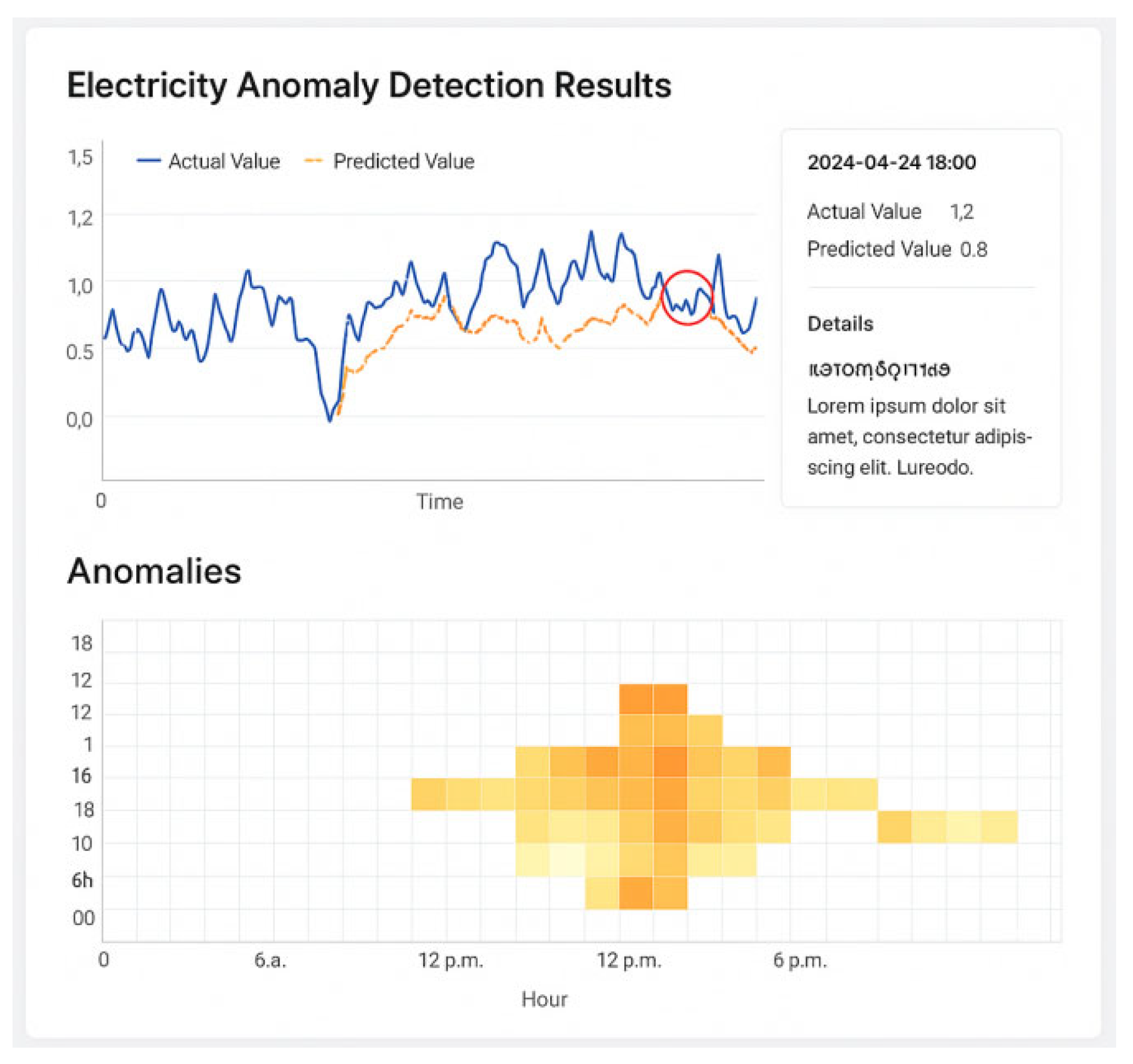
Figure 5. Heat map of consumer electricity data (3 days, 96 points/day).

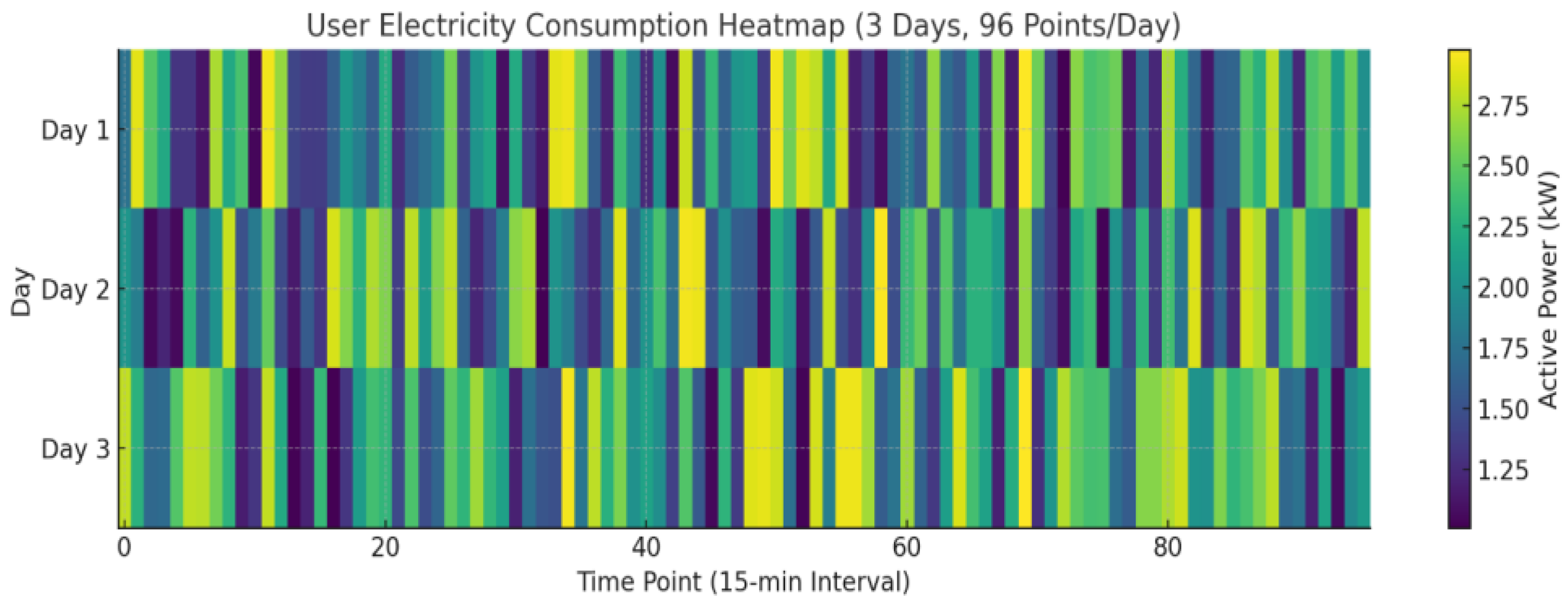
Figure 6. Comparison of different model predictions with anomalous response curves.

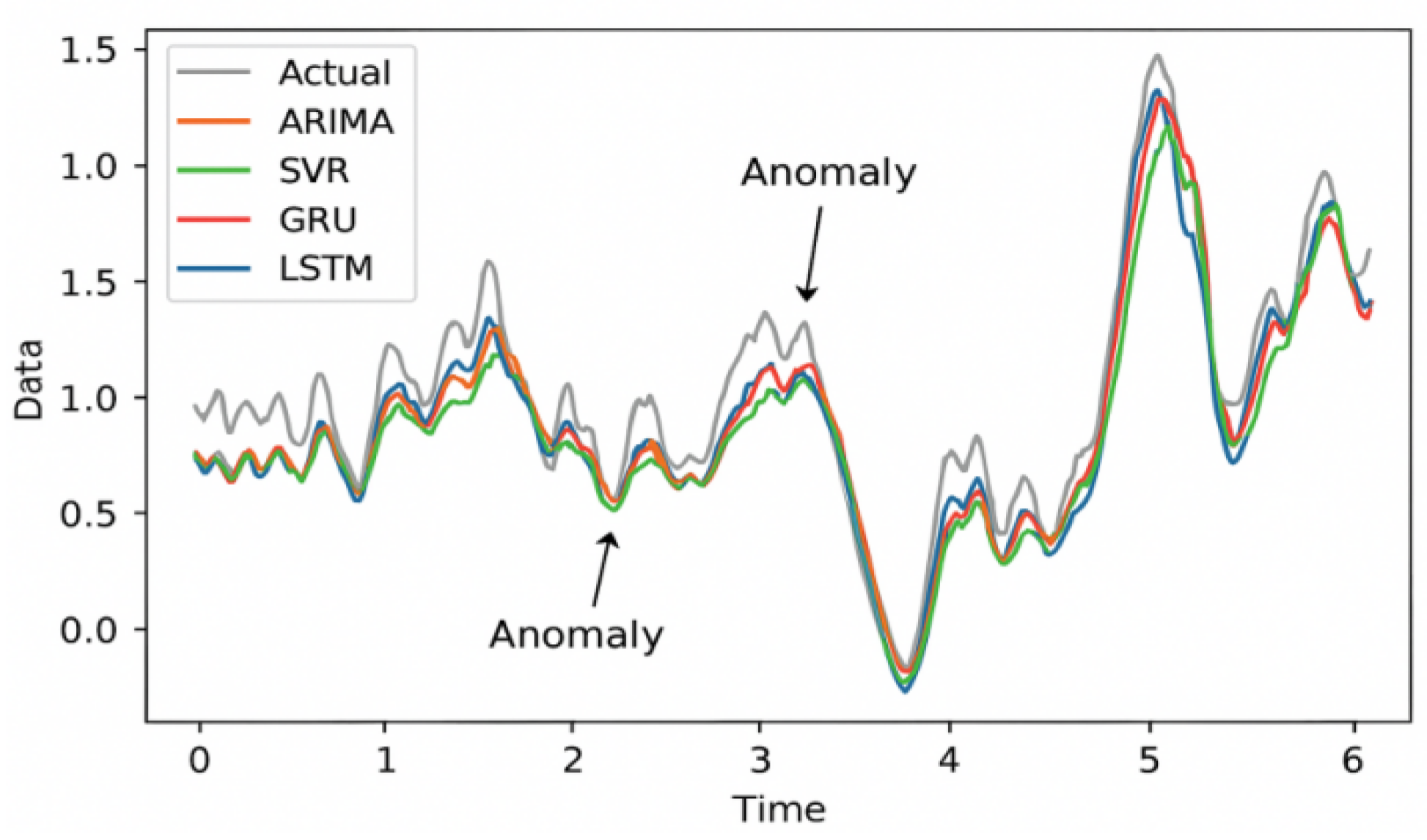
Table 1. residual threshold setting and coverage with different sensitivity factors.

Sensitivity factor k	Threshold setting interval (μ±kσ)	Theoretical coverage (normal distribution)	Description of the criteria for determination
2.0	[μ-2σ,μ+2σ]	95.45%	Balancing misses and false alarms
2.5	[μ-2.5σ,μ+2.5σ]	98.76%	Slightly loose, suitable for regular business
3.0	[μ-3σ,μ+3σ]	99.73%	On the conservative side for sensitive scenarios

Table 2. LSTM model optimization strategy and key parameter settings.

Optimization methods	parameterization	mechanism of action
Early Stopping	patience=5	Preventing training overfitting
L2 regularization	λ=0.001	Suppressing parameter oversizing and enhancing generalization
Dropout	lstm1: 0.2, lstm2: 0.3	Reduce feature dependency and improve robustness
Learning rate decay	Initial 0.001, attenuation factor 0.1	Stabilize convergence and avoid localized shocks

Table 3. description of electricity consumption data collection fields and formats.

Field name	Data Type	Unit (of measure)	Acquisition Frequency
timestamp	datetime	-	Every 15 minutes
voltage	float	V	Every 15 minutes
current	float	A	Every 15 minutes
active_power	float	kW	Every 15 minutes
reactive_power	float	kvar	Every 15 minutes

Table 4. performance comparison of different models on the test set.

Model Type	MSE	MAE	Precision	Recall	F1-score
ARIMA	0.0241	0.102	0.783	0.864	0.821
SVR	0.0176	0.091	0.812	0.841	0.852
GRU	0.0092	0.069	0.901	0.918	0.894
LSTM	0.0084	0.065	0.923	0.949	0.931

Disclaimer/Publisher’s Note: The statements, opinions and data contained in all publications are solely those of the individual author(s) and contributor(s) and not of MDPI and/or the editor(s). MDPI and/or the editor(s) disclaim responsibility for any injury to people or property resulting from any ideas, methods, instructions or products referred to in the content.

© 2025 by the authors. Licensee MDPI, Basel, Switzerland. This article is an open access article distributed under the terms and conditions of the Creative Commons Attribution (CC BY) license (http://creativecommons.org/licenses/by/4.0/).

Copyright: This open access article is published under a Creative Commons CC BY 4.0 license, which permit the free download, distribution, and reuse, provided that the author and preprint are cited in any reuse.