
Submitted:
29 April 2025
Posted:
09 May 2025
You are already at the latest version
Abstract
Electric vehicles are gaining focus and adoption, with new users every day. Their widespread use introduces a new scenario and challenge for the electrical power system due to the high energy storage demands they create. Predicting these loads using artificial neural networks has proven to be an efficient approach for solving time series problems. This work utilizes a multilayer perceptron network through supervised backpropagation training with Bayesian regularization to enhance generalization, reducing overfitting errors. The research aggregates actual consumption data from 200 households and 348 plug-in electric vehicles in the training and forecasting process. To validate the developed method, MAPE was used. Short-term forecasts were made across the four seasons, predicting the total aggregate demand from homes and vehicles for the next 24 hours. The methodology demonstrated significant and relevant results using hybrid training for this problem, with the potential for real-world application.
Keywords:
Electric vehicles
; Artificial neural networks
; Load forecasting
; multilayer perceptron network
; Residential charging
; Backpropagation Bayesian regularization training
1. Introduction
One approach to fostering a cleaner and more sustainable world is to reduce the emission of polluting gases, such as , into the atmosphere. This gas significantly contributes to pollution, which drives climate change, environmental crises, and global instability, raising serious global concerns [1].
The transportation sector is closely linked to a country’s economic foundation and is a significant contributor to emissions [2]. Additionally, the continued prevalence of combustion-based transportation has intensified its impact on climate change and energy crises [3].
The search for alternative and clean energy sources has become an essential option in this context, as pollution from the burning of fossil fuels in the transportation sector is having a significant impact and raising concerns for both the present and near future. As a result, hybrid electric vehicles (HEVs), battery electric vehicles (BEVs), and plug-in hybrid electric vehicles (PHEVs) are becoming increasingly popular and showing promise for a more sustainable future. The focus is on advancing global incentives and policies that accelerate the adoption of electric vehicles (EVs) and promote the decarbonization of transportation [4].
Charging the batteries of plug-in electric vehicles (PEVs) will lead to an increase in electricity demand in distribution networks. This increase is expected to cause voltage drops, thermal overloads, and higher losses [6]. PEVs create high load demand during charging, which could cause the electricity grid to fail in meeting its power delivery capacity, resulting in faults and complications. The main challenge for the electrical system regarding PEVs is how the charging demand can impact the power system, especially during peak consumption times, when vehicle loads are charged in public, private, or residential parking lots [7].
The increasing adoption of EVs will drive a substantial rise in power demand on distribution networks, due to the high and constant need for battery charging. This increase could potentially lead to significant challenges for the electrical system [5], as EV batteries require high power loads during charging, which the existing electrical grid may not always be able to support [6].
These new EV connections present a substantial challenge for the electrical power system, as EVs can be charged in private homes, commercial buildings, companies, and both private and public charging stations [7].
One approach to ensuring that energy demand aligns with consumption is to forecast electrical loads in the energy system, accounting for variations from hours to days, months, and years. This helps guarantee economic, strategic, and other advantages. Forecasting plays a crucial role in directly influencing important operational decisions, such as dispatch, unit commitment, and maintenance scheduling [8].
In this context, ensuring projections and forecasts of electrical loads in the short term has become a timely and relevant topic for concessionaires, the electrical energy market, and academic research. Load forecasting is not easy, as loads correlate not only between hours, days, weeks, or months but also with human behavior and exogenous variables, such as humidity, temperature, and seasons [8].
The introduction of Artificial Neural Networks (ANNs) allows electrical charge forecasting problems to be solved with greater efficiency and accuracy, as this technique learns from historical data and stores certain information for future use [9]. This capability motivated the use of an ANN model in this research. ANN-based learning models are now widely applied in this field, particularly for forecasting charging demand and addressing simultaneous EV charging challenges, among other applications.
This work aims to apply an ANN based on the multilayer feedforward perceptron (MLP) [10] architecture, utilizing hybrid supervised backpropagation training with Bayesian regularization [11], to forecast the total demand generated by EV charging in residential settings. Forecasts were conducted for the next 24 hours of total aggregate demand across each season of the year for comparative analysis.
2. Uncoordinated Residential EV Charging and Impacts
In uncoordinated residential charging, EVs start charging immediately upon being plugged into an outlet, allowing charging to occur at any time, 24 hours a day. These loads exhibit highly random patterns and behavior. Currently, the electricity sector does not recommend this approach and provides little incentive for it, as it does not supply the necessary usage information for scheduled or delayed managed charging, which would optimize EV charging. By delaying the start of charging, EVs can be charged during off-peak times [17].
This charging method does not provide information on energy prices and operates without any control or strategy. EV users can plug in and unplug at any time, or even fully charge the battery whenever they choose [12].
The large-scale integration of EVs into the electrical power system will pose challenges due to the uncoordinated rise in EV connections in households, especially impacting the distribution system. These residential charging loads, combined with EV demand, can significantly increase peak loads, potentially resulting in power shortages, grid congestion, voltage and frequency instability, and failures in electrical components [13].
In this scenario, EV loads require a high level of connectivity for extended periods, often coinciding with peak residential demand. Since the current system is not designed to accommodate high rates of EV adoption, the widespread uncoordinated charging of EVs may adversely affect the distribution, generation, and transmission infrastructure of the electrical power system [14,15].
Generally, energy utilities represent demand through customer profiles based on different usage behaviors, using load curves over time [17]. Each curve corresponds to a distinct profile, such as public, residential, commercial, or industrial [16].
The impacts generated by EVs are substantial due to the high power requirements of aggregate charging and the large-scale adoption of EVs currently underway in the electric mobility sector [18]. The charging of Plug-in Electric Vehicles (PEVs) and Plug-in Hybrid Electric Vehicles (PHEVs) will place additional load on the electrical energy system, increasing residential demand and creating a new total aggregate demand. These vehicles are primarily charged using residential outlets with Level 1 and Level 2 power, often when PEVs are parked in garages in the morning and evening [19].
High connection rates of PEVs in the electrical distribution network create operational challenges [14]. Distribution systems were originally designed to handle conventional load capacities, like residential or commercial loads, based on typical consumer profiles. However, when PEVs are connected, these profiles and the energy demand change significantly due to the high power required over shorter periods for residential charging, as well as for buildings, commercial sites, and public charging stations [20].
3. EV Charging Demand Forecast
EV loads have specific characteristics that differ from residential loads, with unique spatial and temporal distribution profiles. This type of charging requires high power due to its highly periodic and fluctuating nature. EV charging curves exhibit multiple power peaks, particularly within short time intervals throughout the day [21].
In the conventional approach to time series forecasting, historical data and modeling simulations are utilized as the primary sources of information. In this manner, they serve a pivotal function in the domain of forecasting. However, the forecasting of EV-related data is inherently uncertain due to the novel nature of these vehicles and their associated load characteristics. Such load profiles exhibit growth rules and non-stationary and stochastic characteristics. It was observed that, in the case of time series data for which the output exhibits a certain degree of correlation over time, artificial neural networks (ANNs) are a more appropriate choice of modelling approach. This is because ANNs consider previous information in order to make new future projections [22].
The primary challenges associated with forecasting the aggregate charging demand for VEPs can be attributed to several factors, including the inherent volatility of electrical loads, the availability of publicly accessible data, the spatial and temporal distribution characteristics of charging, the diversity of charging modes, the varying rates of penetration of EVs in the network, the uncontrolled growth of charging, and the occurrence of demand spikes. These observations are supported by the findings of reference [22]. As the adoption of electric vehicles (EVs) continues to grow, it is anticipated that the demand for electricity for their charging will have a notable impact on the power grid.
Moreover, the necessity for a consistent and substantial power supply underscores the critical importance of EV charging infrastructure. The high power demand for charging electric vehicles (EVs) imposes significant constraints on the electric grid. In order to address this issue, there is a need to accurately predict the charging load of EVs in conjunction with residential charging. This will assist grid operators in effectively managing power distribution and making informed decisions, as cited in reference [23].
Short-term load forecasting has emerged as a crucial instrument for the intelligent regulation of electric vehicle (EV) charging systems. Nevertheless, such forecasting is not a straightforward undertaking. It necessitates the consideration of various factors, including a comprehensive understanding of the user profile and their consumption patterns. Electric vehicle (EV) charging loads exhibit distinctive characteristics compared to conventional loads. Such loads exhibit spatial and temporal distribution characteristics. The load exerts a considerable demand due to its highly periodic and fluctuating characteristics. The load curves of electric vehicles (EVs) exhibit a number of pronounced energy peaks, particularly over relatively short time periods [22].
The conventional approach to forecasting is based on historical electrical load data, which plays a pivotal role in load forecasting. However, forecasting with EVs presents a number of challenges due to the inherent uncertainties associated with a novel type of load, exhibiting the characteristics previously outlined. The load profiles of EVs exhibit growth rules and characteristics that have yet to be fully elucidated, necessitating extensive investigation [23].
The primary challenges in forecasting the charging demand for electric vehicles (EVs) encompass the characterization of the spatial and temporal distribution of EV loads. This entails the representation of such loads on multi-temporal and spatial scales, as well as the ability to transition between these scales. Additionally, the complexity of EV charging modes and management systems further complicates the prediction of charging demand. The charging of electric vehicles (EVs) occurs in a variety of environments, resulting in the generation of disparate charging profiles [27].
The varying penetration rates of EVs in different regions introduce another layer of complexity, as the rate of EVs plugged in determines the system’s capacity to support and meet load delivery needs. Additionally, the uncontrolled growth of EV charging and the emergence of consumption peaks pose further challenges [27].
4. Multilayer Perceptron Artificial Neural Network
A multilayer feedforward network is characterized by a fully connected structure across all layers. A fundamental property of a multilayer feedforward network is that each neuron in any layer is connected to all other neurons in the previous layer. Consequently, the direction of the signal flow through the network follows a feedforward progression from left to right, propagating in layers [10]. A limitation of multi-layer feedforward networks is that they lack the capacity for feedback. In general, the multilayer feedforward network adds successive values to the inputs and to all neurons in the subsequent hidden and output layers, thereby ensuring that the neurons receive only the input connections [10].
Multilayer perceptron (MLP) [10] ANNs are fully connected layered architecture networks. Neurons in any network layer are always connected to all other neurons in the previous layer, which are interconnected directly in an input layer through weights. This type of network has layers in levels, , an input layer containing one or more neurons, one or several hidden layers, and an output layer containing one or more neurons. Each layer has nodes, and each node is directly connected by weights with nodes in the next layer (Figure 1), being network input signals; N neurons; weights the synaptic weights of neuron N; output signals from N neurons.
MLP transforms its linear inputs through a non-linear activation function (1) [9]:
where f is the activation function of the o-th neuron of the output layer; the output of the h-th hidden layer neuron; the interconnection between the h-th neuron of the hidden layer and the o-th neuron of the output layer, and H the size of the hidden layer.
The transfer function or also called activation defines the type of output of a neuron. The most common activation functions are the relay-type functions, the semi-linear function, the sigmoid function and the hyperbolic tangent [24]. We can exemplify the hyperbolic tangent type sigmoid function (2):
where is the slope of the curve.
5. Backpropagation Training with Bayesian Regularization
The most crucial attribute of a ANN is its capacity to learn from previously presented information, and it can even enhance the information through a learning process conducted by adjusting the weights. When training an ANN, the primary objective is to generate a performance that will produce a low learning error and, most importantly, for this learning to be able to represent an adequate response to new training data. If this occurs, we can conclude that the network has a robust capacity for generalizing data [10].
One of the methods considered effective in improving the generalization of a network training process is regularization. This method involves restricting the values of the weights in an ANN in order to minimize its performance function. The objective of this regularization is to maintain the weights at relatively low values, which allows the network to generate a more smoothly graded output [11].
The (BP) training algorithm with Bayesian regularization (BR) minimizes a combination of quadratic errors and weights and then determines the correct combination to produce training output with high generalization ability [11].
This BR training aims to avoid training overfittings and improve generalization capacity. This training adds a new coefficient to the optimization process, which penalizes the objective function F by increasing the number of [11] coefficients.
In [11] regularization, the objective function F is modified using the sum of the mean squared errors coming from backpropagation, called , and, subsequently, the objective function is increased by the term additional , which is the sum of the squared errors of the network weights bias (3):
with and being the regularization parameters of the objective function, these variables control the training emphasis. While training will focus on minimizing errors in the trained data. And while , training will prioritize minimizing the values of the weights generated by network errors.
The main training challenge is how the terms and are defined to control the objective function. In the Bayesian process, weights are treated as random variables. After obtaining the training data, the weight density function is updated by the Bayes theorem (4).
on what M is the network architecture used; D the training matrix; W the weight matrix; the prior density, representing knowledge of the weights before any data was collected; the likelihood function, which is the probability of a certain event occurring, considering the weights W; and the normalization factor, which guarantees that the total probability is 1.
If it is assumed that the data in the training set is of type Gaussian and its prior distribution for the weights is Gaussian, then probability densities can be written (5) in the following way:
being e .
Replacing these probabilities in (4), we can rewrite the calculation as follows (6):
where is the normalization factor.
In this Bayesian step, the optimal weights maximize the posterior probability . Then, maximizing the posterior probability is equivalent to minimizing the regularized objective function .
5.0.1. Optimization of Regularization Parameters
In this step, the application of Bayes theorem is demonstrated to calculate the optimization of the parameters and of the objective function F (7):
According to the uniform prior density for the regularization parameters and , then maximizing the posterior density is possible by calculating its likelihood function . It is observed that this function is the normalization factor for (4). Assuming that all probabilities have a Gaussian form, the form for the given posterior density (4) is known. It was demonstrated in (6) and it can be solved (4) for the normalization factor (8):
We can observe that the constants and calculated in (5) are known. The only unknown constant is . Caused by Taylor series expansion. One can expand around the minimum point of the posterior density , where the gradient calculation is null. Calculating the normalization constants:
where is a Hessian matrix of the objective function F.
With the result of the calculation in (8) it is possible to calculate the optimal values for and at the minimum point. Taking the derivative with respect to each of the log of (8) and setting them equal to zero will result in (10):
where called the effective number of parameters and N is the total number of parameters in the network. The parameter is a measure of how many neural network parameters are effectively used to minimize the error objective function. It can range from zero to N.
5.0.2. Calculation of the Gauss-Newton Approximation for the Hessian Matrix
BR training requires calculating the Hessian matrix (H) of the objective function for the minimum point . This approximation can be calculated using the Levenberg-Marquardt optimization algorithm to find the minimum point [25].
Training was carried out according to the standard parameters of the Bayesian regularization training algorithm in the Matlab 2015b software (toolboxes) with the nntool function [11].
The default value for the maximum number of validation failures is set to infinity. This ensures that the training process continues until the optimal balance between errors and weights is achieved. The optimization function relies on the Jacobian matrix for calculations, where the performance metric is the sum of squared errors. Consequently, this training process uses the Mean Squared Error (MSE) as its performance evaluation function.
Bayesian regularization takes place within the Levenberg-Marquardt algorithm. The backpropagation error known as backpropagation is used to calculate the Jacobian of performance in relation to the weight variables and the bias X [30]. Each variable is adjusted according to the Levenberg-Marquardt algorithm, described in the equation 11:
where:
- E: all errors;
- I: identity matrix;
- : parameter of Marquardt.
The five steps required for Bayesian optimization of the regularization parameters, with the Gauss-Newton approximation for the H matrix, can be simplified as follows:
- Initialization of , and the weights. We choose , and use the Nguyem-Widrow method to initialize the weights [28]. After the first training step, the parameters of the objective function are recovered from the initial configuration;
- Execution of one stage of the Levenberg-Marquardt algorithm to minimize the objective function ;
- Calculation of the effective number of parameters using the Gauss-Newton approximation for the matrix H available in the Levenberg-Marquardt training algorithm , where J is the Jacobian matrix of the errors of the training set [29];
- Calculation of new estimates for the parameters of the objective function and ;
- Execution of steps 2 and 4 until convergence.

Table 1.
TRAINING PARAMETERS AND MLP.
| Parameters | Values | |
|---|---|---|
| Activation function | Hyperbolic tangent | |
| Number of neurons per layer | ( 5-6-2-1-1 ) | |
| Number of hidden layers | 3 | |
| Number of neurons per hidden layer | (6-2-1) | |
| Performance function | Mean square error | |
| BP learning rate | 0.005 | |
| Bayesian regulation | 0 | |
| Bayesian regulation | 1 | |
| Maximum number of iterations | 1000 | |
| Performance goal | 0 | |
| Marquardt Decrease Factor () | 0.1 | |
| Marquardt increase factor () | 10 | |
| Maximum Marquardt value () | 1x10¹⁰ | |
| Maximum fault value ahead | 500 | |
| Minimum gradient value | 1x10 −9 | |
| Training time | ∞ |
The adaptive value of is increased by the Marquardt growth factor until the change in the 11 equation results in a reduced performance value. This change is made by decreasing the decrement factor of the Marquardt parameter . Bayesian regularization training will be interrupted as soon as any of these conditions occur:
- The maximum number of training epochs has been reached;
- The maximum time has been exceeded;
- Objective performance is minimized;
- The value of the performance gradient exceeds the chosen minimum value;
- exceeds the maximum validation failure value.
6. Materials and Methods
To apply the proposed method, the data set proposed is in reference [19]. The data are from 200 private residences in the Midwest region of the United States (USA). The household composition included 502 individuals and 348 EVs. The load profiles were measured regarding electrical power in Watts (W), with a resolution of 10 minutes over one year. VEPs with 60% load and Pluggable Hybrid Electric Vehicles (PHEV) with 40% load were considered, all charged with a level 1 plugged with a power of 1920 W.
6.0.3. Pre–Processing and Processing
As the original data has a resolution of 10 minutes in the very-short term, it was decided to group the measurements for a resolution of 1 hour in the short term. All home measurements and all EV charging were added together each hour, forming measurements from 00:00 to 23:00. The transformation was done by reducing 144 measurements (10-minute resolution) to 24 measurements (1-hour resolution) each day.
The data was separated into two demands: the first represented by residential demand and the second by EV demand. A single column containing all measurements was generated for each demand by adding the 200 homes and 348 vehicles, forming vectors of 8760×1, data from the two consumptions over one year. The total demand (11) was obtained by the sum of all respective loads every hour, day, and month between the two demands, residential and EVs (Figure 2):
where is the total aggregate demand for forecasting; total residential demand; total EV demand.
6.1. Separation of Training and Testing Data Sets
When separating the training and testing data sets, total aggregate demand was used. The total set made up of 8760 measurements was divided into the 4 seasons of the year, for the purpose of comparisons and analysis of seasonality. In this way, 4 forecasts were proposed for the next 24 hours, one for each season of the year. The input and test matrices are composed of the variables:
- Days: = day variables;
- Weeks: = variables for the weeks from Monday to Sunday;
- Months: = variables from the months of January to December;
- Times: = variables in hours in the 24-hour period;
- Loads : [total aggregate demand] = load variables referring to the hour in Watts.
The ANN output set is composed of the total aggregate demand variable, with representing the load measurements for the following hour , in Watts.
The dataset was separated into 83% for training and 17% for testing. The dimensions of the datasets are presented in Table 1.
Table 2.
DIMENSIONS OF TRAINING AND TESTING SETS.
| Sets/ | Training | Test | ||
|---|---|---|---|---|
| Stations | Input | Output | Input | Output |
| Spring | ||||
| Summer | ||||
| Fall | ||||
| Winter | ||||
6.2. Configuration and Architecture of the ANN
Initially, it was decided to divide the 1-year database into the year’s four seasons, as climate change has direct links to consumption patterns and profiles of EVs and homes. With this, predictions become more realistic and perform better. To obtain a better configuration for the ANN architecture, exhaustive tests were carried out by varying the number of hidden layers and the number of neurons in the hidden layers. The best configuration found was the one with six neurons in the first hidden layer, 2 in the second hidden layer, and 1 in the third hidden layer. The hyperbolic tangent activation function was used.
6.3. Prediction Performance Evaluation
7. Results
Figure 3, Figure 4, Figure 5 and Figure 6 present the results obtained with the methodology proposed in this research.
The software used for modeling, training, and prediction was Matlab 2023b. In training, the data set is divided randomly by default; even when splitting the set into 83 %, the algorithm divides this value in random order to make the training process more robust without being associated with a single answer.
Tests were carried out on the configurations of the hidden layers and their number of neurons, and it was observed that the best configuration of the network is with three hidden layers. This configuration was the best performing due to the accuracy and stability of the training response. It was noted that, with fewer than three hidden layers, the network loses precision, demonstrating a limitation of the network in training, and with more than three layers, the network loses training stability. The architecture of the proposed model achieved a significant improvement in the learning process, finding the best configuration of the numbers of neurons and hidden layers.
Table 2 presents the MAPE results obtained for each season of the year.
Table 3.
FORECAST RESULTS BY SEASON OF THE YEAR.
| Results | spring | Summer | Fall | Winter |
|---|---|---|---|---|
| MAPE(%) | 4,5042 | 5,1180 | 3,6487 | 3,3624 |
8. Discussion
It was possible to observe that using only backpropagation training the response is not satisfactory, that is the reason to use a hybrid training with Bayesian Regularization is used. With the union of the two training sessions, the network obtained a significant improvement in results, as Bayesian regularization determines the probability of an event happening given the saved learning. With these improvements, the proposed architecture and technique increase its effectiveness.
In the spring forecast, the biggest errors were found during the night, between 7 pm and 9 pm, with average errors of . This is due to the peak generated by EVs during this period. It was also seen that in the morning, at precisely 9 am, the network showed an error of .
It was observed that the highest load peaks due to the penetration of EVs are found in the morning (between 7 am and 12 pm) and also at night (between 6 pm and 9 pm). With these peaks in residential demand, the maximum errors are found at these times. It was observed that between 1 pm and 6 pm the forecasts had low errors, caused by the low charge of the EVs.
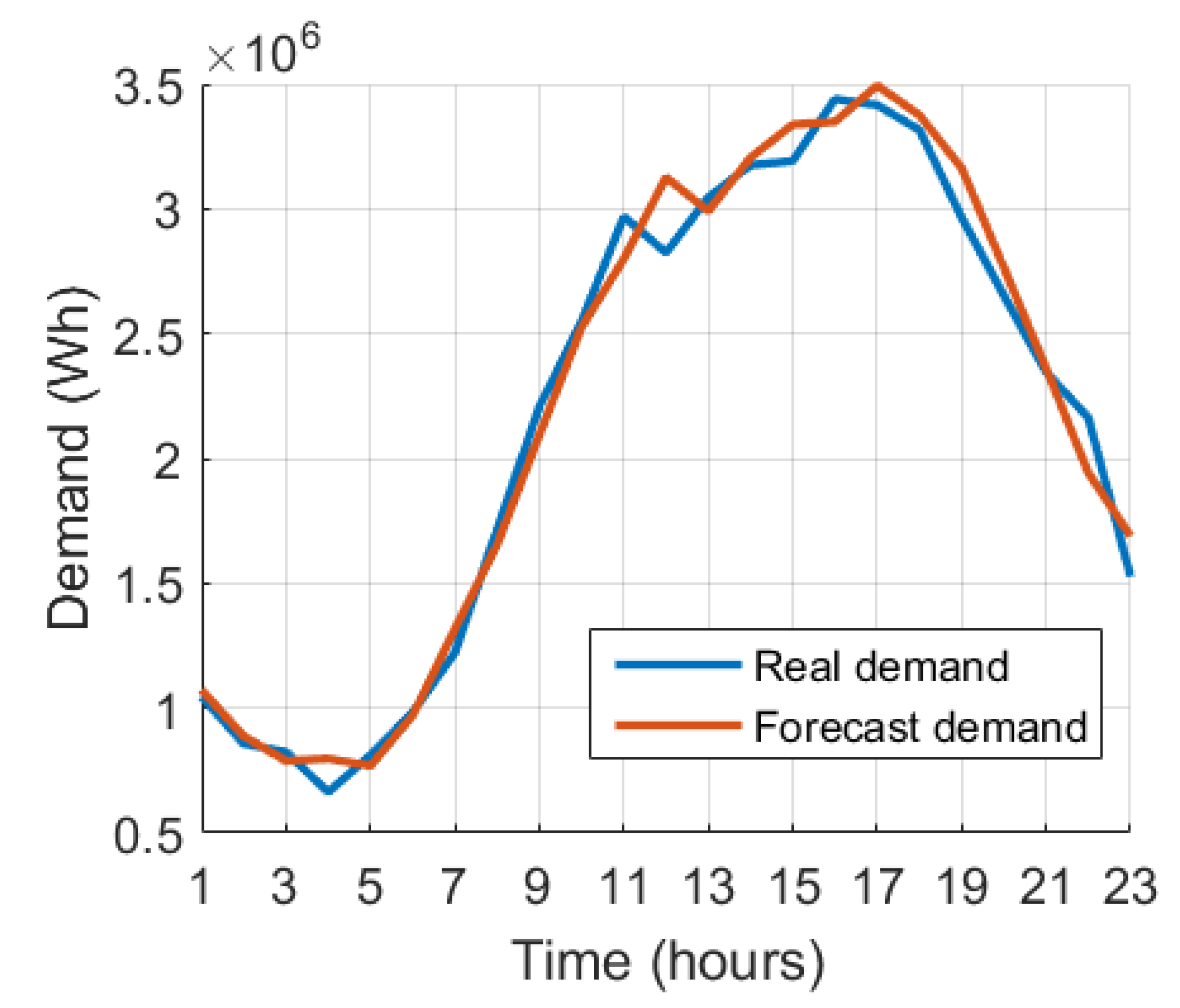
The forecast for summer presented the biggest errors when compared to the other three seasons, with three very pronounced error times: in the morning with a error (largest error), in the lunch period with of error and at night with of error (between 9 and 10 pm).
For the winter period, the network obtained the lowest errors compared to the other seasons. However, it obtained a maximum error of in the morning peak hour and at this point the network was optimistic, that is, it overestimated the demand at the predicted time.
The fall forecast resulted in the MAPE being just above the winter forecast. At peak loading times the maximum error was .
It is also observed that due to the amount of trained data from the winter and summer seasons being greater than the others, this division generated greater maximum errors than the others, arround 15.934% in the winter and 20.228% in the summer.
The growth in the adoption of EVs in residential charging had a major impact on the electrical power system. The forecast of total loading demand presents itself as an important strategic tool in a scenario with a broad growth trend and with great openness for exploration and investigation.
The MLP network and the proposed training showed good generalization capacity, with satisfactory results and fast convergence, with training time between 5 and 15 seconds and 200 to 500 iterations. The use of three hidden layers was of great importance for the training generalization process, increasing the quality of the results. The proposed model showed an improvement in learning due to hybrid training, which resulted in more realistic responses, satisfying the need for reliable predictions with more precision and robustness.
9. Conclusions
Total demand forecasting presented itself as a promising option for future projections, having the ability to estimate new demands based on EV loads added to residential load, instead of just making forecasts in EVs. In this way, the ANN learned the behavior of residential loads, EVs and both being used simultaneously.
The proposed methodology presented promising answers to a topic in high and rapid expansion, relatively recent and with great potential for practical application in future research. The proposal, due to its efficiency and reliability in results, has the possibility of being implemented in order to assist in the development of a robust strategy, preparing the power system for new EV penetration rates. This work also has the potential to assist in the development of strategies for smart charging, optimizing the EV charging process.
Funding
The authors would like to thank the Coordination for the Improvement of Higher Education Personnel - Brazil (CAPES) - Funding code 001 and the CNPq number 302948/2022-8 (National Council for Scientific and Technological Development.
Data Availability Statement
All electrical power demand profiles used in this study, including residential energy demand and level 1 electric vehicle charging, are available for free download. “MDPI Research Data Policies” at https://data.nrel.gov/submissions/69.
References
- ``International Energy Agency. Global EV Outlook.” (2021). https://www.iea.org/reports/global-evoutlook-2021.
- EPA, “Multipollutant comparison.,” 2016. 05 December. 2020.
- Y. Fan, C. Guo, P. Hou. Impact of electric vehicle charging on power load based on tou price. Energy and Power Engineering 2013, 05, 1347–1351. [Google Scholar] [CrossRef]
- H. Cui, D. Hall, and N. Lutsey. Update on the global transition to electric vehicles through 2019,” tech. rep. Internacional Council on Clean Transportation 2020, 07. [Google Scholar]
- A. Raskin and S. Saurin, “The emergence of hybrid vehicles,” tech. rep., Alliance Bernstein’s Research on Strategic Change, 2006.
- P. Papadopoulos, S. Skarvelis-Kazakos, I. Unda. Electric vehicles’ impact on british distribution networks. IET Electrical Systems in Transportation 2012, 2, 91–102. [Google Scholar] [CrossRef]
- K. Clement-Nyns, E. Haesen, and J. Driesen. The impact of charging plug-in hybrid electric vehicles on a residential distribution grid. Power Systems, IEEE Transactions on 2010, 25, 371–380. [Google Scholar] [CrossRef]
- H. Hippert, C. Pedreira, and R. Souza. Neural networks for short-term load forecasting: A review and evaluation. IEEE Transactions on Power Systems 2001, 16, 44–55. [Google Scholar] [CrossRef]
- S. Haykin, Neural Networks: A Comprehensive Foundation. USA: Prentice Hall PTR, 2nd ed., 1998.
- M. Minsky and S. Papert, Perceptrons: An Introduction to Computational Geometry. Cambridge, MA, USA: MIT Press, 1969.
- D. J. C., MacKay. A practical bayesian framework for backprop networks. Neural Computation 1992, 4, 448–472. [Google Scholar]
- D. J. C., MacKay. Electric vehicles and the electric grid: A review of modeling approaches, Impacts, and renewable energy integration. Renewable and Sustainable Energy Reviews 2013, 19, 247–254. [Google Scholar]
- Légifrance., “Loi n° 2015-992 du 17 août 2015 relative à la transition énergétique pour la croissance verte.,” 2015. Acessado: 28 jan. 2021.
- J. A. P. Lopes, F. J. Soares, and P. M. R. Almeida, “Integration of electric vehicles in the electric power system,” Proceedings of the IEEE, vol. 99, pp. 168–183, 01 2011.
- A. Schroeder, “Modeling storage and demand management in power distribution grids,” Applied Energy, vol. 88, no. 12, pp. 4700–4712, 2011.
- H. L. Willis, Power Distribution Planning Reference Book. CRC Press, 2004.
- S. Shafiee, M. Fotuhi-Firuzabad, and M. Rastegar, “Investigating the impacts of plug-in hybrid electric vehicles on power distribution systems,” IEEE Transactions on Smart Grid, vol. 4, pp. 1351–1360, 09 2013.
- G. Putrus, P. Suwanapingkarl, D. Johnston, E. Bentley, and M. Narayana, “Impact of electric vehicles on power distribution networks,” in 2009 IEEE Vehicle Power and Propulsion Conference, pp. 827 – 831, IEEE, 10 2009.
- M. Muratori, “Impact of uncoordinated plug-in electric vehicle charging on residential power demand,” Nature Energy, vol. 3, pp. 193–201, 01 2018.
- C. Roe, A. Meliopoulos, J. Meisel, and T. Overbye, “Power system level impacts of plug-in hybrid electric vehicles using simulation data,” in 2008 IEEE Energy 2030 Conference, pp. 1–6, IEEE, 11 2008.
- J. Zhu, Z. Yang, J. Guo, Y.and Zhang, and H. Yang, “Short-term load forecasting for electric vehicle charging stations based on deep learning approaches,” Applied Sciences (Switzerland), vol. 9, p. 1723, 04 2019.
- G. Chunlin, Q. Wenbo, W. Li, D. Hang, H. Pengxin, and X. Xiangning, “A method of electric vehicle charging load forecasting based on the number of vehicles,” in International Conference on Sustainable Power Generation and Supply (SUPERGEN), pp. 1–5, IET, 09 2012.
- A. K. Karmaker, M. A. Hossain, H. R. Pota, A. Onen, and J. Jung, “Energy management system for hybrid renewable energy-based electric vehicle charging station,” IEEE Access, vol. 11, pp. 27793–27805, 2023.
- B. Krose, P. van der Smagt, and Smagt, “An introduction to neural networks,” J Comput Sci, vol. 48, 01 1993.
- F. Foresee and M. Hagan, “Gauss-newton approximation to bayesian learning,” Proceedings of International Conference on Neural Networks (ICNN’97), vol. 3, pp. 1930–1935, 08 1997.
- D. C. Park, M. A. El-Sharkawi, R. J. Marks, L. E. Atlas, and M. J. Damborg, “Electric load forecasting using an artificial neural network,” IEEE Transactions on Power Systems, vol. 6, no. 2, pp. 442–449, 1991.
- CHUNLIN, G.; et al. A method of electric vehicle charging load forecasting based on the number of vehicles. In: INTERNATIONAL CONFERENCE ON SUSTAINABLE POWER GENERATION AND SUPPLY (SUPERGEN 2012), 2012, Hangzhou. Anais[...]. [S.l.]: Hangzhou, China, 2012. p. 1–5.
- NGUYEN, D.; WIDROW, B. Improving the learning speed of 2-layer neural networks by choosing initial values of the adaptive weights. In: IJCNN INTERNATIONAL JOINT CONFERENCE ON NEURAL NETWORKS. Anais[...]. [S.l.]: Oxford, 1990. v. 3, p. 21–26.
- FORESEE, F. D.; HAGAN, M. Gauss-newton approximation to bayesian learning. In: PROCEEDINGS OF INTERNATIONAL CONFERENCE ON NEURAL NETWORKS (ICNN’97). Anais[...]. [S.l.]: Houston, 1997. v. 3, p. 1930–1935.
- RUMELHART, D.; GEOFFREY, E. H.; WILLIAMS, R. J. Learning representations by back-propagating errors. London. 1986, 323, 533–536. [Google Scholar]
Figure 1.
Multilayer perceptron architecture.
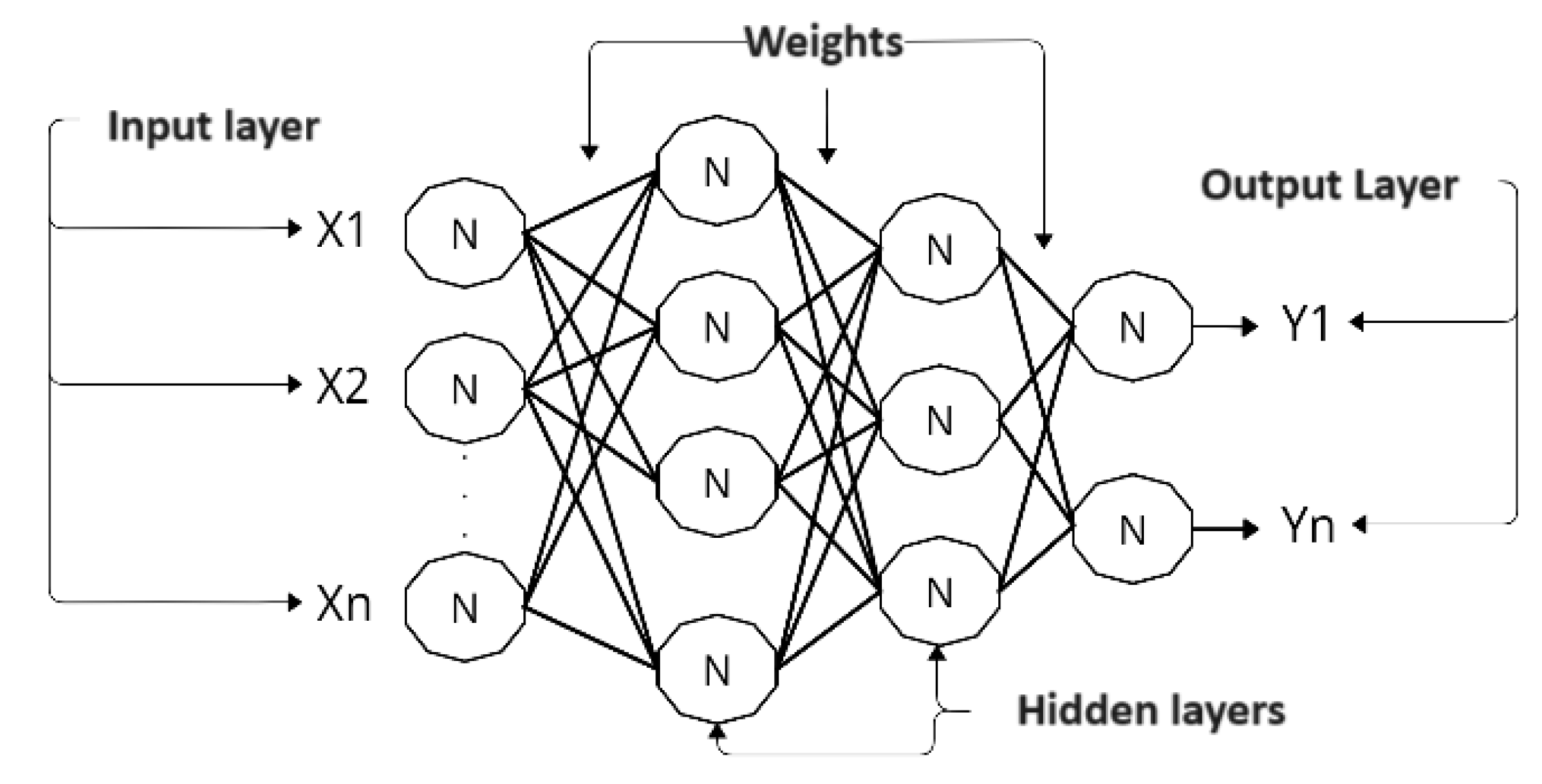
Figure 2.
Comparison between demands.
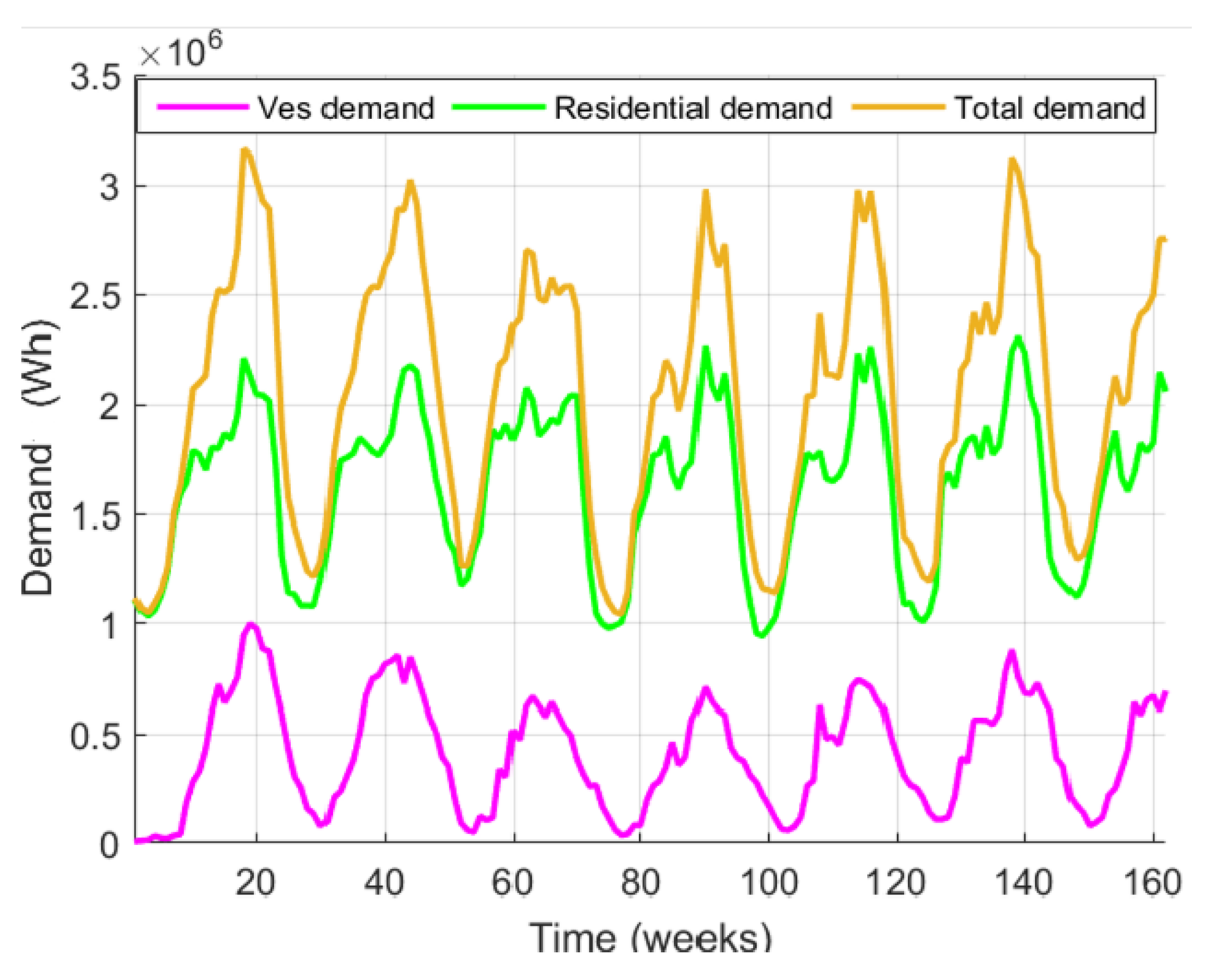
Figure 3.
24-hour winter demand forecast.
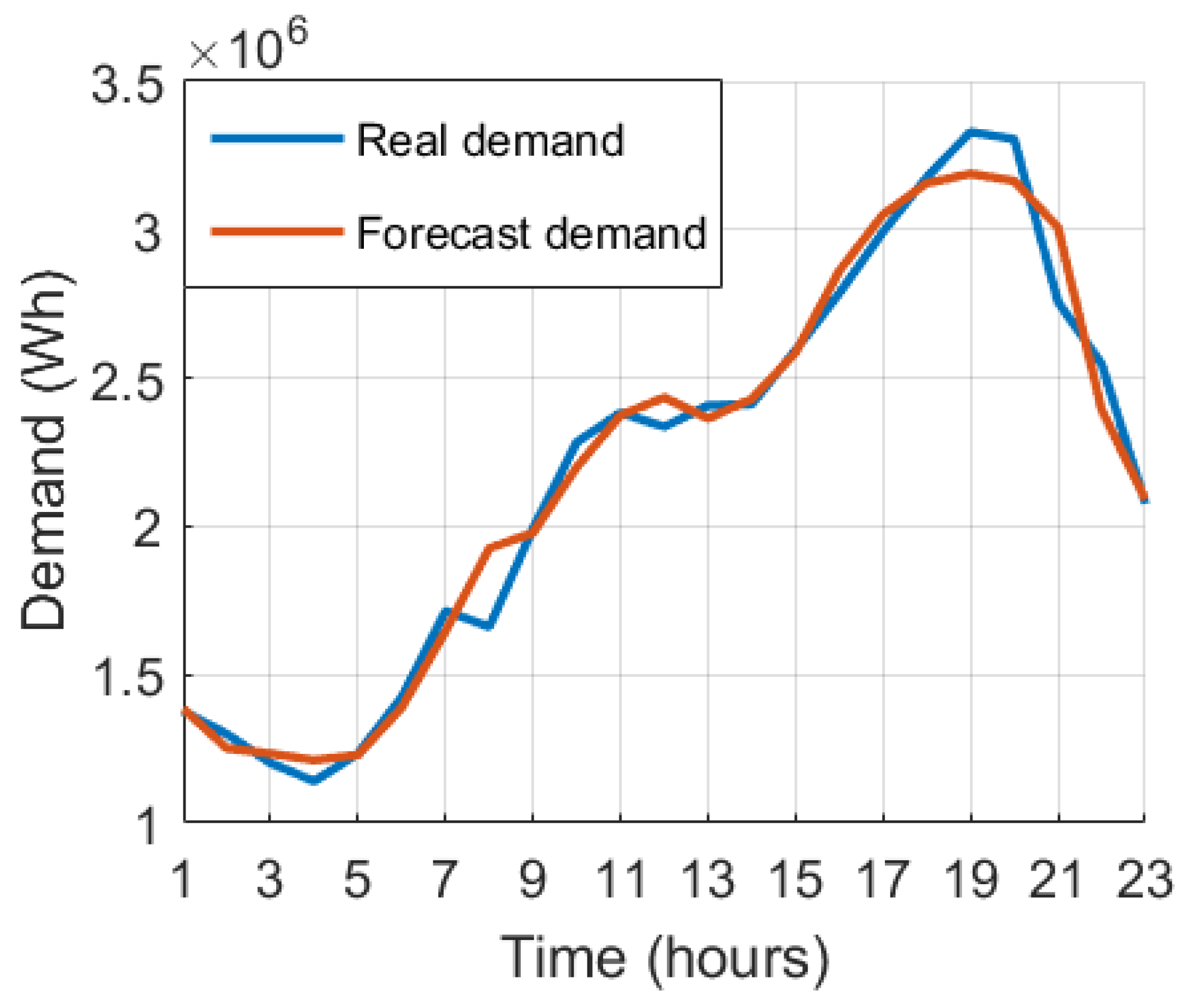
Figure 4.
24-hour fall demand forecast.
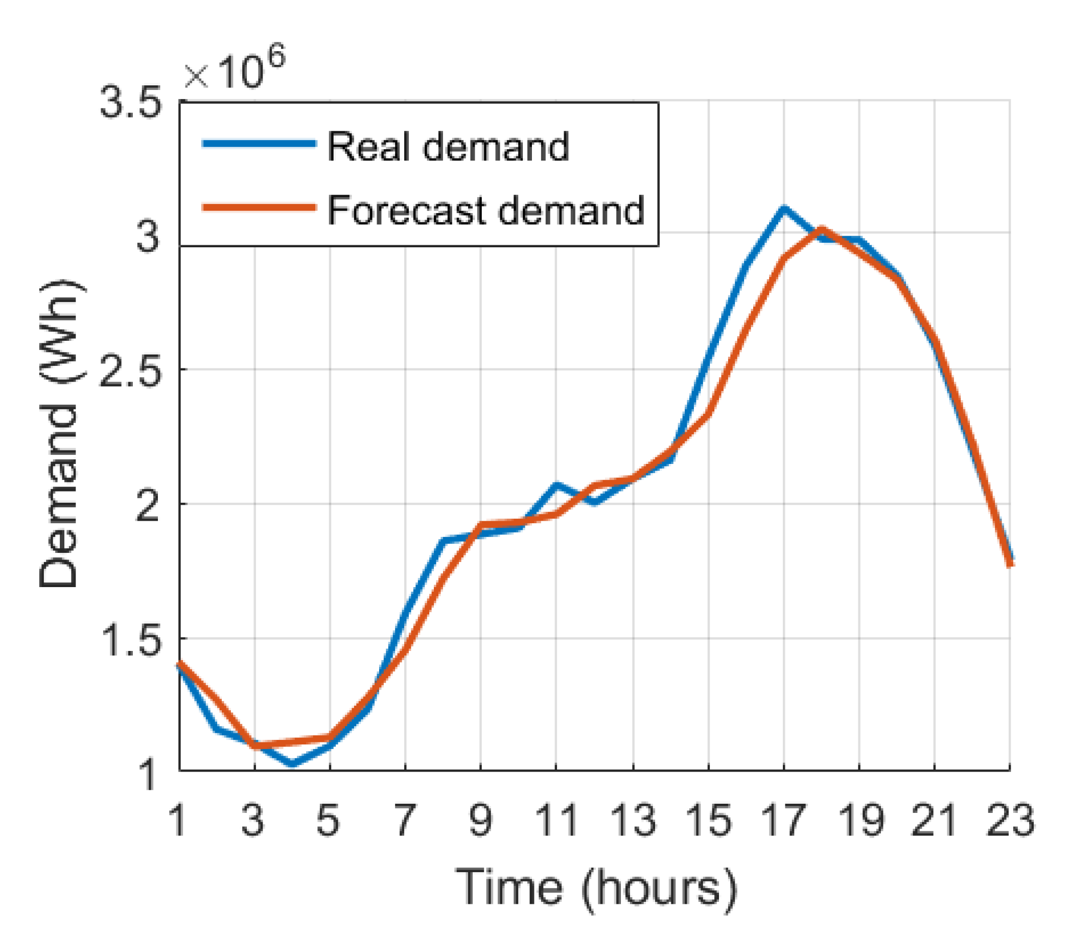
Figure 5.
24-hour spring demand forecast.
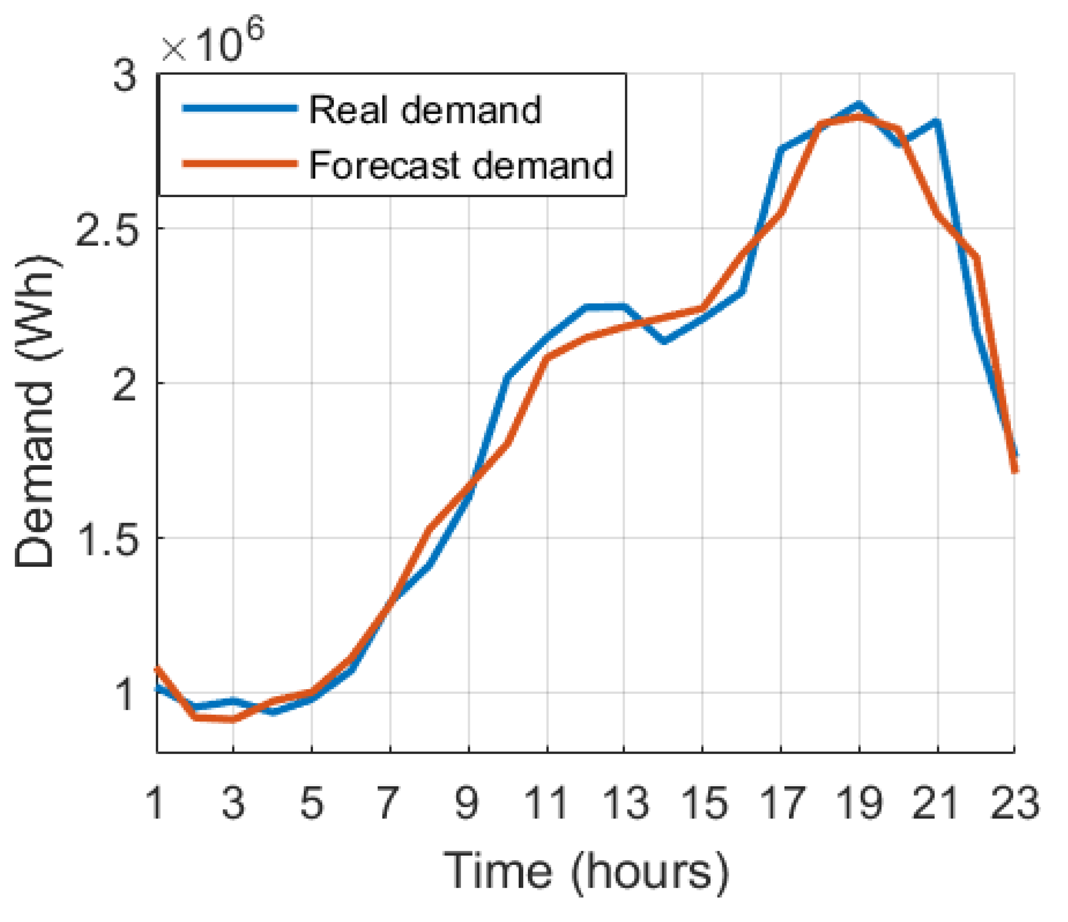
Figure 6.
24-hour summer demand forecast.
Disclaimer/Publisher’s Note: The statements, opinions and data contained in all publications are solely those of the individual author(s) and contributor(s) and not of MDPI and/or the editor(s). MDPI and/or the editor(s) disclaim responsibility for any injury to people or property resulting from any ideas, methods, instructions or products referred to in the content. |
© 2025 by the authors. Licensee MDPI, Basel, Switzerland. This article is an open access article distributed under the terms and conditions of the Creative Commons Attribution (CC BY) license (http://creativecommons.org/licenses/by/4.0/).
Copyright: This open access article is published under a Creative Commons CC BY 4.0 license, which permit the free download, distribution, and reuse, provided that the author and preprint are cited in any reuse.


