Submitted:
18 September 2024
Posted:
19 September 2024
You are already at the latest version
Abstract
Quadruped robots possess significant mobility in complex and uneven terrains due to their outstanding stability and flexibility, making them highly suitable in rescue missions, environmental monitoring, and smart agriculture. With the increasing use of quadruped robots in more demanding scenarios, ensuring accurate and stable state estimation in complex environments has become particularly important. Existing state estimation algorithms relying on multi-sensor fusion, such as those using IMU, LiDAR, and visual data, often face challenges on non-stationary terrains due to issues like foot-end slippage or unstable contact, leading to significant state drift. To tackle this problem, this paper introduces a state estimation algorithm that integrates an Invariant Extended Kalman Filter (InEKF) with a disturbance observer, aiming at estimating the motion state of quadruped robots on non-stationary terrains. Firstly, foot-end slippage is modeled as a deviation in body velocity and explicitly included in the state equations, allowing for a more precise representation of how slippage affects the state. Secondly, the state update process integrates both foot-end velocity and position observations to improve the overall accuracy and comprehensiveness of the estimation. Lastly, a foot-end contact probability model, coupled with an adaptive covariance adjustment strategy, is employed to dynamically modulate the influence of the observations. These enhancements significantly improve the filter's robustness and the accuracy of state estimation in non-stationary terrain scenarios. Experiments conducted with the Jueying Mini quadruped robot on various non-stationary terrains show that the enhanced InEKF method offers notable advantages over traditional filters in compensating for foot-end slippage and adapting to different terrains.
Keywords:
quadruped robots
; invariant extended Kalman filter
; state estimates
; non-stationary terrain
1. Introduction
Quadruped robots are advanced robotic systems inspired by four-legged animals. Compared to other types of mobile robots, quadruped robots have excellent stability and flexibility, capable of walking on various complex and uneven terrains such as sand, grass, gravel roads, and even slippery surfaces. These capabilities make quadruped robots highly promising for applications in rescue missions [1], environmental monitoring [2], and smart agriculture [3]. With the advancement of technology, quadruped robots are increasingly being used in various demanding scenarios, such as mountainous areas, forests, and post-disaster rubble environments. To ensure the stability and reliability of robots in complex environments, precise state estimation becomes particularly important.
State estimation algorithms based on multi-sensor fusion are widely used in quadruped robots, incorporating external sensors like LiDAR, cameras, and GPS, as well as proprioceptive sensors such as IMUs and joint encoders [4]. While external sensors provide rich environmental information, they have limitations; for example, cameras perform poorly in low-light or low-texture environments, LiDAR's accuracy degrades under smoke or dust, and GPS signals can be disrupted in indoor or urban canyon settings [5]. In contrast, proprioceptive sensors, which rely on joint kinematics and IMU data, are unaffected by such environmental factors and offer higher measurement frequencies, enabling fast and precise control of quadruped robots. Therefore, it is crucial to explore state estimation methods based on proprioceptive sensors such as IMUs and joint encoders. IMUs provide high-frequency acceleration and angular velocity data, while joint encoders offer precise measurements of joint angles and speeds. Combining these sensors enables accurate motion state estimation in complex environments, particularly when external sensors fail or are limited. This approach enhances the autonomy, robustness, and reliability of quadruped robots in diverse scenarios.
State estimation methods for legged robots date back to 2005 when Lin [6] developed an approach based on leg kinematic information for a hexapod robot. This method required the robot to maintain a tripod gait with three legs always in contact with a flat terrain. In 2006, Lin [7] further proposed fusing leg odometry with IMU data to improve state estimation during tripod gait running. Since then, state estimation for legged robots has garnered significant attention. Bloesch [8] introduced a quadruped robot state estimation method using an Extended Kalman Filter (EKF), incorporating leg contact points into the filter's state variables and using forward kinematics to estimate leg contact positions and body pose. Camurri [9] developed a legged odometry method without contact sensors, using ground reaction forces to determine the reliability of leg contact and weight each leg's contribution to body velocity. However, due to inconsistencies between EKF's positive feedback and observation information, the filter may diverge. To address this, Hartley [10] proposed a contact-aided Invariant Extended Kalman Filter (InEKF) based on invariant observer theory, showing better performance compared to the traditional quaternion-based EKF.
The aforementioned methods assume stable, slip-free foot-end contact between legged robots and the ground. However, on slippery or soft terrains such as snow, mud, or sand, foot-end slippage occurs, making stable contact challenging. This introduces non-Gaussian errors that accumulate over time, causing unbounded drift. To address this, Ting [11] treated slippage in foot-end observations as outliers and used a weighted least squares method to mitigate their impact on the EKF. Similarly, Bloesch [12] replaced the EKF with an Unscented Kalman Filter (UKF) and applied an outlier rejection method to manage occasional slippage. Jenelten [13] developed a probabilistic slip detector using a Hidden Markov Model, allowing robots to walk on slippery surfaces through impedance control and friction adjustment. However, this approach does not completely resolve pose estimation drift. To reduce drift from slippage, some methods fuse external sensor observations. Wisth [14] proposed a factor graph optimization-based state estimation method that tightly integrates visual features, inertial data, and kinematic constraints. This method was further extended to incorporate LiDAR observations and an online-estimated linear velocity deviation term to minimize drift in legged odometry [4]. Kim [15] introduced a state estimator for quadruped robots based on a pre-integrated foot velocity factor, which does not rely on precise contact detection or fixed foot positions, showing strong performance on uneven and slippery terrains. However, factor graph-based methods use measurements along the entire trajectory for smoothing, which limits their update rates for real-time control. To address this, Teng [16] integrated camera observations into the Invariant Extended Kalman Filter (InEKF) to enhance state estimation on slippery terrains. Fink [17] combined a Global Exponential Stability (GES) nonlinear attitude observer with legged odometry, ensuring consistently bounded speed estimation and reducing drift in unobservable position estimates.
Recently, advancements in computational hardware (e.g., GPUs) have enabled the training and deployment of complex deep learning models, encouraging researchers to develop learning-based slip detection and state estimation methods. Rotella[18] proposed a method using fuzzy clustering to learn contact probabilities for humanoid robots, which, when integrated into a basic state estimation framework, can significantly reduce estimation errors. Buchanan[19] developed a deep neural network to learn motion patterns from IMU data, and when combined with traditional legged odometry, it substantially reduces drift in proprioceptive state estimation. Yang[20] applied neural networks to train weight functions for foot-end forces and legged odometry states, enhancing observation accuracy. However, learning-based methods face challenges such as poor model interpretability and limited generalization. Supervised models require large amounts of labeled data, which is often difficult to obtain, while unsupervised methods treat slip detection as a classification task, limiting the ability to observe slip velocity.
Inspired by [4], we consider modeling slip velocity as a deviation term of speed and explicitly incorporating it into the state equations to reduce pose drift caused by slip through slip velocity estimation. To meet real-time requirements, we opted for a filtering-based method. The Invariant Extended Kalman Filter (InEKF), developed based on invariant observer theory, has been successfully applied in simultaneous localization and mapping (SLAM) [21] and aided inertial navigation systems [22] in recent years. Its symmetry ensures that the estimation error satisfies the "log-linear" autonomous differential equation on the Lie algebra of the corresponding Lie group in the system dynamics. Thus, it is possible to design a nonlinear observer or state estimator that exhibits strong convergence within an attraction domain independent of the system trajectory. Yu [23] presented a similar approach for wheeled platforms, mainly using speed observations from encoders. We have extended this to legged robot platforms. Unlike wheeled platforms, speed observations from encoders at the foot-end are less reliable than those from wheel encoders. To address this issue, we incorporate the contact point positions of each leg into the filter state variables and consider both foot-end position and velocity observations in the observation equation, making the filter more suitable for legged robots.
The main contributions of this paper are as follows:
1. Model foot-end slippage caused by legged robot motion on unstable terrain as a deviation term of body velocity, reducing drift caused by foot-end slippage through velocity deviation estimation.
2. Develop a real-time RI-EKF state and slip estimator for quadruped robots by fusing foot-end velocity and position observations.
3. Validate the mathematical derivation and the proposed state estimator's effectiveness through experimental results using the Jueying Mini robot on multiple unstable terrains.
2. Theoretical Backround
The Assume a matrix Lie group denoted as , with its corresponding Lie algebra denoted as . Let represent the isomorphism that maps elements in the tangent space at the identity element to their corresponding matrix representations in . The exponential mapping of the Lie group is denoted by and is represented as , where is the usual exponential mapping of matrices. A system that evolves over time on a Lie group can be represented by the dynamics: ,represents the system state, and is usually used to denote the estimated state.
Definition 1.
(Right-invariant and left-invariant errors) The right-invariant and left-invariant errors between the two trajectories and are defined as follows:
where is an arbitrary element of the group .
Definition 2.
(Adjoint map) Let be a matrix Lie group with its Lie algebra denoted as . For any , the adjoint map is a linear map that satisfies . Furthermore, the matrix representation of the adjoint map is denoted by .
Theorem 1.
A system is group-affine, if for all , its dynamics satisfies:
where is the identity matrix. If a system is group-affine, then its right-invariant and left-invariant error dynamics are independent of the trajectory and satisfy:
Define a matrix of size such that for any the function holds. Let be the solution to the following linear differential equation:
Theorem 2.
Consider any two trajectories defined by (4) and (5) with a left-invariant and right-invariant error, respectively. For any initial error , if , then for all ,the nonlinear estimation error can be accurately recovered by the linear differential equation (6), where .
3. System Model
3.1. State Equation
Our state estimator can estimate the state variables of the robot's motion in the world coordinate system , which include the robot's orientation , robot's position , robot's velocity , and the positions of the four feet , , , .To consider the impact of end-effector slippage on state estimation, we use an anti-slippage observer idea, introducing a bias term modeled as a drift velocity and explicitly incorporating it into the state equations. These state variables form a group in , hence we represent the state variables of our InEKF model as:
To better understand the content, we adopt the following simplified notation:
Similar to [23], we describe the slippage velocity using an autoregressive model, modeling the slippage velocity as an exponentially decaying variable:
The IMU provides the following measurements
The measurement of foot position primarily relies on the angular measurements from joint encoders, and the joint encoder measurements are
Based on the IMU measurement model and the foot-end contact model, the system's dynamic model is:
Rewrite the above model in matrix form,
where , It can be proven that the deterministic system dynamics satisfy the group affine property (3). According to Theorem 1, the left-invariant and right-invariant error dynamics are autonomous and evolve independently of the system state. The system's right-invariant error is:
Theorem 2 further explains the logarithmic linear property of invariant errors. If is defined as
Then the invariant error satisfies the following linear system:
Using first-order approximation to linearize yields:
Substituting into the expression for , we drive:
Based on these computations, the prediction step of the right-invariant extended Kalman filter (EKF) can be derived. The state estimate is denoted as , and the covariance matrix is obtained using the Riccati equation:
where .
3.2. Measurement Model
According to the forward kinematics of the quadruped robot, the position of the foot relative to the body coordinate system is given by:
The velocity of the foot is composed of the velocity generated by the joint rotation and the velocity of the body motion
Transform and into the world coordinate system , we can obtain the foot velocity in the world coordinate system:
When the foot is in stable contact with the ground without slipping, , that is:
Assuming that the joint encoder is affected by Gaussian white noise with a covariance matrix of , i.e. we can derive the following observation model:
Therefore, when in stable contact, there exist the following two observations:
The first equation represents the observation of the foot position of the quadruped robot, denoted as where ,,,.The second equation represents the observation of the body velocity of the quadruped robot, denoted as , where ,, , . Hartley [10] used position as the observation in bipedal robots, while Teng [16] used velocity as the observation. In practice, these two observations can be considered together. Using the moving pose as an example, the observation error is defined as:
Substituting into (32) , we have
Note that for each foot's data observation, except for the first row, all other elements are 0. Let be the term where all 0 elements are removed:
Combining all foot position observations, we have:
Similarly, for velocity observations, we have:
By merging velocity observations with position observations, we get:
3.3. Considering Unstable Contact and Slipping
The above model assumes that all four feet are in stable contact with the ground. In practice, however, the quadruped robot’s feet may be airborne during walking, and on many uneven or slippery terrains, the feet may make unstable contact. When the feet are airborne or in unstable contact, the foot positions calculated by the state-space model do not conform to this assumption. To address this issue, we use the foot contact probability model proposed in [9] to determine the probability of stable contact between the feet and the ground.
Using this contact probability, we can combine the basic velocities generated by each leg to obtain the body velocity and use it as an observation of the body velocity.
Considering the sliding velocity of the foot, we have
where represents the error in the body velocity, which includes the error generated by each foot velocity observation. To correctly compute the covariance matrix of consider the consistency between each foot velocity and the ground impact. For each axis , the variance at a given moment can be computed as:
where is the average absolute difference in the ground reaction force in the z axis between the current and previous contact times. is the baseline standard deviation of velocity, is the standard deviation of stance phase foot velocity contribution for the r-th elements. is a factor that balances consistency and the impact of collision forces, while is a normalization factor to normalize the typical velocity error difference at the same moment.
For the observation of foot position, since the foot may be in a hovering state or in unstable contact, the estimated foot position obtained through the state-space model might be unreliable. By dynamically adjusting the noise covariance of the foot contact using the formula below, the impact of unstable or non-contact states on state estimation can be mitigated:
where L is a sufficiently large scalar. The final observation model accounting for unstable contact and sliding is as follows:
An observation equation of the form is obtained. Based on the definition of right-invariant error, the update steps for InEKF are as follows:
4. Experimental Results and Analysis
To validate the effectiveness of the proposed algorithm, experiments were conducted on three different terrains using the Jueying Mini quadruped robot. The Jueying Mini quadruped robot is equipped with an IMU and 12 joint encoders, all with a measurement frequency of 166 Hz. The IMU provides measurements of angular velocity and linear acceleration, while the joint encoders provide measurements of joint angles, joint torques, and joint angular velocities. Table 1 presents the corresponding noise parameters. The experimental terrains include typical outdoor rugged slopes, shallow grass, and deep grass, as shown in the Figure 1.
4.1. Contact Probability Calculation
We use the phase information of the foot-end as the true value of the contact state between the foot-end and the ground. The parameters , in Equation (38) are used to compute the contact force between the foot-end and the ground by minimizing the energy:
Considering that the foot-end starts to touch the ground and prepares to leave the ground, the position of the foot-end always undergoes some displacement. An appropriate adjustment of the parameter reduces the sensitivity of the model to input variation, thereby making the fluctuation of the foot-end contact probability smoother. Figure 2 illustrates the scenario where the quadruped robot’s foot slips during contact with the ground,and Figure 3 presents the final results, showing the probability model for the right front foot slipping
4.2. Algorithm Evaluation
Due to the absence of a motion capture system in outdoor areas, we used the LiDAR SLAM method, which performs relatively well in outdoor environments, with LIO-SAM’s computed pose information serving as the ground truth. The experimental results are shown in the figures. Figure 4 presents the trajectory estimates results of various methods for the quadruped robot across three different terrains. We compared a total of five methods: the traditional quaternion-based Kalman filter method (Q-EKF)[8], InEKF with only velocity updates[16], InEKF with only position updates, and the proposed method considering and not considering velocity bias. For the methods [16] and [10], when the foot is in the contact phase, it is determined to be in stable contact with the ground, while the remaining methods employ the proposed contact probability judgment and covariance adjustment strategy. The results from the figure show that the proposed method is closer to the true trajectory.
The trajectories of different methods under various terrains were evaluated using the EVO tool, with the results shown in Table 2. The evaluation metrics include Absolute Trajectory Error (ATE) and Relative Pose Error (RPE), where ATE and RPE measure position error (in meters) and rotation error (in radians), respectively.
Table 2 shows that proposed method (PM with Vel Bias) outperforms other methods in ATE and RPE across all terrains, especially on rugged slopes and shallow grass, where its position error (ATE) and attitude error (RPE) are the lowest, at 0.4572 meters and 0.0345 radians (for rugged slopes position error) and 0.3431 meters and 0.0367 radians (for shallow grass position error), respectively. This indicates that this method offers higher accuracy and robustness in scenarios with velocity bias compensation. In contrast, InEKF with Vel update shows larger errors in most terrains, particularly in deep grass, where the ATE reaches 3.3818 meters and RPE is 1.3146 radians, demonstrating its sensitivity to errors in complex terrains. However, the method shows good stability and accuracy in RPE rotational error performance across various terrains, particularly on shallow grass and rugged slopes. These results indicate that velocity observation plays a crucial role in maintaining low rotational errors. Combining velocity observations with other methods (such as position observation) holds promise for achieving more robust attitude estimation. PM without Vel Bias also shows relatively stable performance in shallow grass and deep grass, especially in position error, suggesting that the strategy of removing velocity bias can be beneficial for trajectory estimation accuracy under certain terrain conditions. The QEKF method performs between other methods but has the lowest rotation error (RPE) on shallow grass, at 0.0367 radians, indicating its advantage in handling certain types of attitude changes. Overall, the experimental results show that the proposed method provides the best performance in most cases.
5. Conclusions
To address the state estimation drift issue caused by unstable foot contact in non-stationary terrains for quadruped robots, we propose an improved Invariant Extended Kalman Filter (InEKF) method. This method models foot-end sliding as a bias term in body velocity and integrates both foot-end velocity and position observations into the observation equation. By using foot-end contact probability assessment and adaptive covariance adjustment strategies, it effectively improves the state estimation accuracy of quadruped robots in complex outdoor environments. Experimental results show that, compared to several existing methods(such as Q-EKF and InEKF with single observation update), our method exhibits lower Root Mean Square Error (RMSE) across multiple unstable terrains and demonstrates significant advantages in position and attitude estimation. This method offers a new approach to the state estimation problem of quadruped robots on non-stationary terrains and suggests further optimization of the filtering algorithm for application in more complex environments in the future.
References
- Cruz Ulloa, C.; Del Cerro, J.; Barrientos, A. Mixed-reality for quadruped-robotic guidance in SAR tasks. Journal of Computational Design and Engineering. 2023, 10, 1479–1489. [Google Scholar] [CrossRef]
- Halder, S.; Afsari, K.; Serdakowski, J. Real-time and remote construction progress monitoring with a quadruped robot using augmented reality. Buildings 2022, 12, 2027. [Google Scholar] [CrossRef]
- Hansen, H.; Yubin, L.; Ryoichi, I.; Takeshi, O.; Yoshihiro, S. Quadruped Robot Platform for Selective Pesticide Spraying. In Proceedings of the 2023 18th International Conference on Machine Vision and Applications (MVA), Hamamatsu, Japan, 23–25 July 2023. [Google Scholar]
- David, W.; Marco, C.; Maurice, F. VILENS: Visual, Inertial, Lidar, and Leg Odometry for All-Terrain Legged Robots. IEEE Trans. Robot. 2023, 39, 309–326. [Google Scholar] [CrossRef]
- Junwoon, L.; Ren, K.; Mitsuru, S.; Toshihiro, K. Switch-SLAM: Switching-Based LiDAR-Inertial-Visual SLAM for Degenerate Environments. IEEE Robot. Autom. Lett. 2024, 9, 7270–7277. [Google Scholar] [CrossRef]
- Lin, P.; Komsuoglu, H.; Koditschek D., E. A leg configuration measurement system for full-body pose estimates in a hexapod robot. IEEE Trans. Robot. 2005, 21, 411–422. [Google Scholar] [CrossRef]
- Lin, P.; Komsuoglu, H.; Koditschek D, E. Sensor data fusion for body state estimation in a hexapod robot with dynamical gaits. IEEE Trans. Robot. 2006, 22, 932–943. [Google Scholar] [CrossRef]
- Bloesch, M.; Hutter, M.; Hoepflinger M., A. State estimation for legged robots: Consistent fusion of leg kinematics and IMU. In Robotics: Science and Systems VIII. 2013. Nicholas, R., Paul N., Eds.; MIT Press: Cambridge, MA, USA, 2013; pp. 17–24. [Google Scholar] [CrossRef]
- Camurri, M.; Fallon, M.; Bazeille, S. Probabilistic contact estimation and impact detection for state estimation of quadruped robots. IEEE Robot. Autom. Lett. 2017, 2, 1023–1030. [Google Scholar] [CrossRef]
- Hartley, R.; Jadidi, M. G.; Grizzle J., W. Contact-aided invariant extended Kalman filtering for legged robot state estimation. Int. J. Robot. Res. 2020, 39, 402–430. [Google Scholar] [CrossRef]
- Ting, J.; Theodorou, E. A. A Kalman filter for robust outlier detection. In Proceedings of the 2007 IEEE/RSJ International Conference on Intelligent Robots and Systems, San Diego, CA, USA, 29 October–2 November 2007. [Google Scholar]
- Michael, B.; Christian, G.; Péter, F.; Marco, H. Mark, A. State estimation for legged robots on unstable and slippery terrain. In Proceedings of the 2013 IEEE/RSJ International Conference on Intelligent Robots and Systems, Tokyo, Japan, 3–7 November 2013. [Google Scholar]
- Jenelten, F.; Hwangbo, J.; Tresoldi, F. ; Dynamic locomotion on slippery ground. IEEE Robot. Autom. Lett. 2019, 4, 4170–4176. [Google Scholar] [CrossRef]
- Wisth, D.; Camurri, M.; Fallon, M. Robust legged robot state estimation using factor graph optimization. IEEE Robot. Autom. Lett. 2019, 4, 4507–4514. [Google Scholar] [CrossRef]
- Kim, Y.; Yu, B.; Lee, E.M. STEP: State estimator for legged robots using a preintegrated foot velocity factor. IEEE Robot. Autom. Lett. 2022, 7, 4456–4463. [Google Scholar] [CrossRef]
- Teng, S.; Mueller, M.W.; Sreenath, K. Legged robot state estimation in slippery environments using invariant extended kalman filter with velocity update. In Proceedings of the 2021 IEEE International Conference on Robotics and Automation(ICRA), Xi'an, China, 30 May–5 June 2021. [Google Scholar]
- Fink, G.; Semini, C. Proprioceptive sensor fusion for quadruped robot state estimation. In Proceedings of the 2020 IEEE/RSJ International Conference on Intelligent Robots and Systems (IROS), Las Vegas, NV, USA, 24 October 2020-24 January 2021. [Google Scholar]
- Rotella, N.; Schaal, S.; Righetti, L. Unsupervised contact learning for humanoid estimation and control. In Proceedings of the 2018 IEEE International Conference on Robotics and Automation (ICRA), Brisbane, QLD, Australia, 21–25 May 2018. [Google Scholar]
- Buchanan, R.; Camurri, M.; Dellaert, F. Learning inertial odometry for dynamic legged robot state estimation. In Proceedings of the 5th Annual Conference on Robot Learning, London, UK, 8–11 November 2021. [Google Scholar]
- Yang, S.; Yang, Q.; Zhu, R. State estimation of hydraulic quadruped robots using invariant-EKF and kinematics with neural networks. Neural Comput. Appl. 2024, 36, 2231–2244. [Google Scholar] [CrossRef]
- Zhang, T.; Wu, K.; Song, J. Convergence and consistency analysis for a 3-D invariant-EKF SLAM. IEEE Robot. Autom. Lett. 2017, 2, 733–740. [Google Scholar] [CrossRef]
- Zhang, H.; Xiao, R.; Li, J. A High-Precision LiDAR-Inertial Odometry via Invariant Extended Kalman Filtering and Efficient Surfel Mapping. IEEE Trans. Instrum. Meas. 2024, 73, 1–11. [Google Scholar] [CrossRef]
- Yu, X.; Teng, S.; Chakhachiro, T. Fully proprioceptive slip-velocity-aware state estimation for mobile robots via invariant kalman filtering and disturbance observer. In Proceedings of the 2023 IEEE/RSJ International Conference on Intelligent Robots and Systems (IROS), Detroit, MI, USA, 1–5 October 2023. [Google Scholar]
- Grupp, M. evo: Python package for the evaluation of odometry and SLAM. Available online: https://github.com/MichaelGrupp/evo (accessed on 17 September 2024).
Figure 1.
Test Environments.
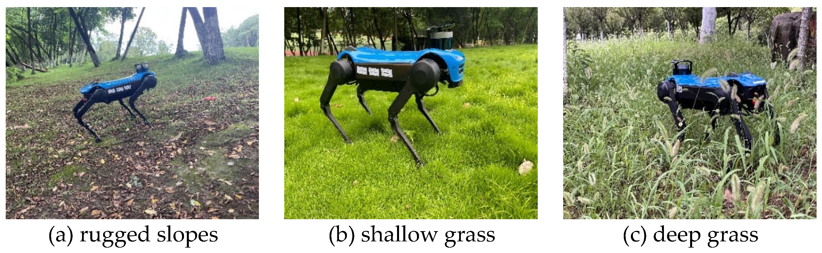
Figure 2.
Foot Slipping Scenarios of a Quadruped Robot During Ground Contact.
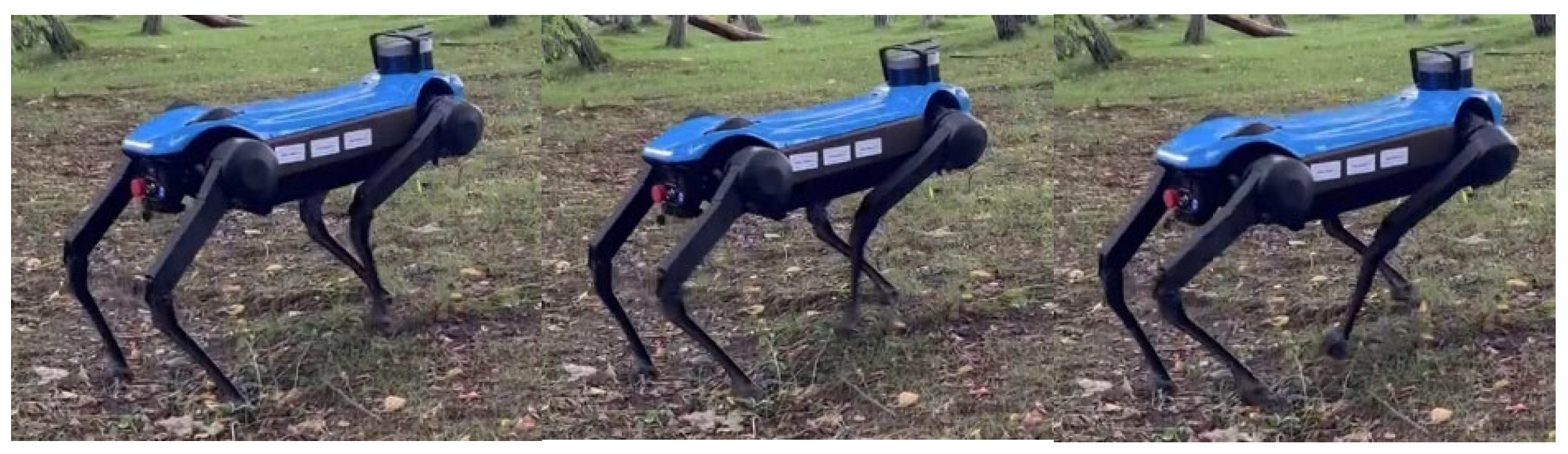
Figure 3.
Estimation of foot contact probability during unstable contact events, with (a) representing the right front leg and (b) the left rear leg.
Figure 3.
Estimation of foot contact probability during unstable contact events, with (a) representing the right front leg and (b) the left rear leg.
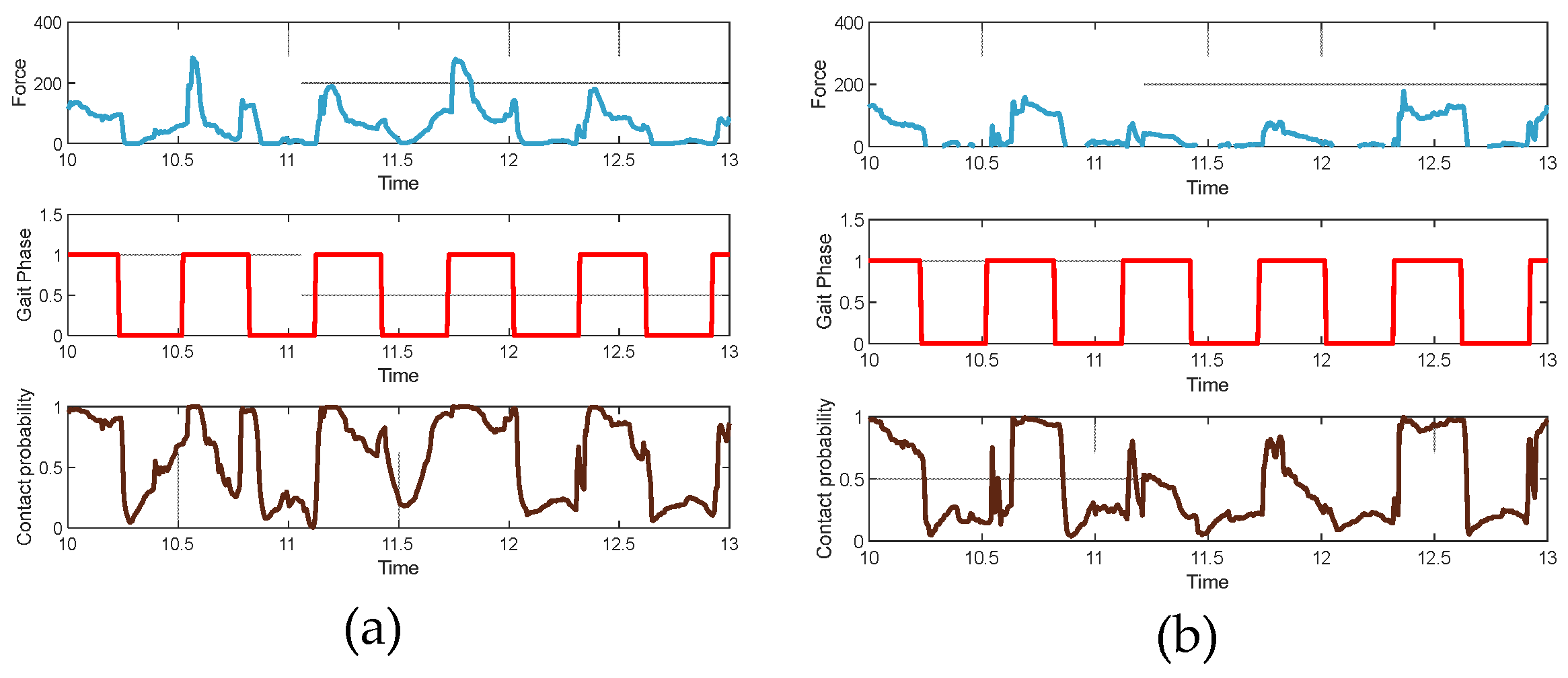
Figure 4.
Trajectory estimates of the quadruped robot under different terrains, with (a) depicting the trajectory estimate for rugged slope terrain, (b) for shallow grass terrain, and (c) for deep grass terrain.
Figure 4.
Trajectory estimates of the quadruped robot under different terrains, with (a) depicting the trajectory estimate for rugged slope terrain, (b) for shallow grass terrain, and (c) for deep grass terrain.
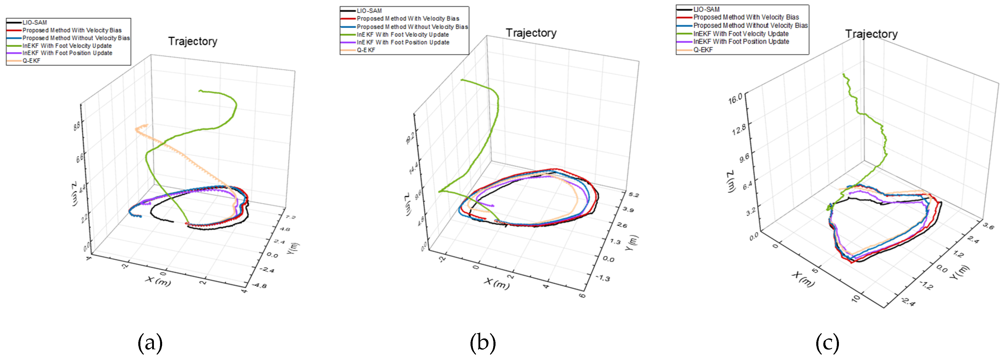

Table 1.
Noise Parameters and initial Covariances.
| Measurement Type | Noise std. dev | State Variable | Initial Covariance |
|---|---|---|---|
| Gyroscope | 0.1 rad/s | Robot Orientation | 0.03 rad |
| Accelerometer | 0.1 m/s2 | Robot Velocity | 0.01 m/s |
| Foot Encoder Pos | 0.01 m | Robot Position | 0.01 m |
| Foot Encoder Vel | 0.1 m/s | Robot Slip Velocity | 0.01 m/s |
| Disturbance Process | 5 m/s |
Table 2.
RMSE evaluation of different state estimation methods for quadruped robots on various terrains.
Table 2.
RMSE evaluation of different state estimation methods for quadruped robots on various terrains.
| Terrain | Method | ATE RMSE | RPE RMSE | ||
|---|---|---|---|---|---|
| Position(m) | Rotation(rad) | Position(m) | Rotation(rad) | ||
| Rugged Slopes | QEKF | 1.3459 | 1.0541 | 0.0654 | 0.0385 |
| InEKF with Vel update | 1.5898 | 2.8388 | 0.0743 | 0.0395 | |
| InEKF with Pos update | 0.4704 | 0.2185 | 0.0633 | 0.0358 | |
| PM without Vel Bias | 0.4666 | 0.1628 | 0.0601 | 0.0358 | |
| PM with Vel Bias | 0.4572 | 0.1626 | 0.0601 | 0.0345 | |
| Shallow Grass | QEKF | 0.7893 | 0.4661 | 0.0697 | 0.0367 |
| InEKF with Vel update | 2.3747 | 3.0528 | 0.0665 | 0.0368 | |
| InEKF with Pos update | 0.6525 | 0.3039 | 0.0626 | 0.0655 | |
| PM without Vel Bias | 0.3501 | 0.1238 | 0.0393 | 0.0630 | |
| PM with Vel Bias | 0.3431 | 0.1261 | 0.0391 | 0.0641 | |
| Deep Grass | QEKF | 0.5993 | 0.2867 | 0.0628 | 0.0558 |
| InEKF with Vel update | 3.3818 | 1.3146 | 0.0797 | 0.0452 | |
| InEKF with Pos update | 0.7552 | 0.3526. | 0.0653 | 0.0522 | |
| PM without Vel Bias | 0.6920 | 0.3228 | 0.0646 | 0.0506 | |
| PM with Vel Bias | 0.5289 | 0.2035 | 0.0601 | 0.0498 | |
Disclaimer/Publisher’s Note: The statements, opinions and data contained in all publications are solely those of the individual author(s) and contributor(s) and not of MDPI and/or the editor(s). MDPI and/or the editor(s) disclaim responsibility for any injury to people or property resulting from any ideas, methods, instructions or products referred to in the content. |
© 2024 by the authors. Licensee MDPI, Basel, Switzerland. This article is an open access article distributed under the terms and conditions of the Creative Commons Attribution (CC BY) license (http://creativecommons.org/licenses/by/4.0/).
Copyright: This open access article is published under a Creative Commons CC BY 4.0 license, which permit the free download, distribution, and reuse, provided that the author and preprint are cited in any reuse.


